Article

Tool Wear Condition Monitoring Based on Improved Symmetrized Dot Pattern Enhanced Resnet18 Under Small Samples

1
School of Business Management, Jiaxing Nanhu University, Jiaxing 314001, China
2
Jiaxing Key Laboratory of Intelligent Manufacturing and Operation & Maintenance of Automotive Parts, Jiaxing Nanhu University, Jiaxing 314001, China
3
School of Photovoltaic Modern Industry, Jiaxing Nanhu University, Jiaxing 314001, China
4
Laser and Optoelectronic Intelligent Manufacturing Research Institute, Wenzhou University, Wenzhou 325035, China
5
School of Mechatronics and Transportation, Jiaxing Nanyang Polytechnic Institute, Jiaxing 314003, China
*
Authors to whom correspondence should be addressed.
Lubricants 2025, 13(11), 503; https://doi.org/10.3390/lubricants13110503 (registering DOI)
Submission received: 28 September 2025 / Revised: 3 November 2025 / Accepted: 10 November 2025 / Published: 17 November 2025

Abstract

Timely and effective identification of the tool wear condition is crucial for ensuring the machining quality of CNC machine tools. In most industrial scenarios, the cost of sample collection is high, so only a small number of samples are available for model training, making it difficult for the existing tool wear condition monitoring (TCM) methods based on deep learning to achieve high performance. To address this problem, this paper proposes a TCM method based on the improved symmetric dot pattern (SDP) enhanced ResNet18. Firstly, the time series sample data is converted into grayscale matrices through SDP, the correlation coefficient between the grayscale matrices is calculated, and the optimal parameter combination of SDP is determined according to the objective of minimizing the correlation coefficient. Then, the cutting force signal is converted into a lobe diagram of the optimized SDP to enrich the sample feature information. Next, the SDP lobe diagram is input into ResNet18 for few-shot learning. The results of a series of TCM experiments demonstrate that the proposed method is significantly superior to the STFT and GAF based methods.

1. Introduction

At present, manufacturers in many industries such as aerospace, automobile, and precision machinery demand high requirements for the machining accuracy and surface quality of components. As cutting tools play the central role in cutting processes, their condition directly affects the machining quality [1]. Traditional methods for judging the condition of cutting tools mostly rely on the experience and intuitive feeling of operators. For example, whether a cutting tool is still usable can be determined by observing the shape of chips generated during the cutting process, examining the surface quality of workpieces, setting a threshold for the number of processed workpieces, and so on. These methods are highly subjective and tend to be conservative. As a result, many cutting tools are replaced before reaching the failure threshold, increasing the cost of machining necessarily [2]. Therefore, developing more effective methods for accurate and automatic tool wear condition monitoring (TCM) is of great significance for ensuring the machining quality of components [3,4,5].
TCM is a highly challenging job. Over the past 30-odd years, many scholars have conducted research on cutting tool wear condition monitoring and developed a host of wear condition monitoring methods. These methods can be divided direct monitoring methods and indirect monitoring methods. Direct monitoring methods make use of industrial cameras and machine vision algorithms to observe and measure the wear condition of cutting tools directly [6]. Methods of this type are convenient to use, but their implementation requires expensive high-precision cameras, and the monitoring quality can be affected by the fluid and debris flying in all directions during the machining process [2,7]. Unlike direct monitoring methods, indirect monitoring methods monitor the sensing signals, related to tool condition during the machining process, and use feature extraction techniques and machine learning models to infer the wear condition of each tool, such as cutting force [8], vibration [9], and temperature [10,11]. Although indirect monitoring methods cannot reflect the processing state as the direct monitoring methods do, they do not require halting the machining process and have the advantages of good real-time performance and strong anti-interference ability, which has attracted the attention of many researchers [12,13,14,15,16]. With the development of deep learning technology, the indirect monitoring method has become a hot spot of research, and a host of monitoring methods that can yield good results have been proposed [17,18,19]. Yang et al. proposed to process cutting force signals using the multivariate variational mode decomposition (MVMD) method and extract features using the improved multi-scale permutation entropy method, and used a one-dimensional convolutional neural network (1D CNN) to classify tool wear conditions [20]. Cheng et al. designed a multi-scale DenseNet-GRU fusion model and introduced an attention mechanism to optimize the mapping between signal features and wear conditions, achieving an 18% reduction in prediction errors in milling experiments [21]. Dai et al. improved the CNN structure by combining a long short-term memory network and convolutional kernel, and achieved end-to-end wear recognition using cutting force signals as inputs [22]. Their proposed method can be applied to online monitoring of wear conditions. Li et al. developed a lightweight CNN model to identify wear conditions in real-time based on cutting force signals [23]. These models can achieve excellent classification performance in certain scenarios, but they have the following limitations when dealing with small sample data:
(1)
Heavy reliance on data. The above-mentioned models require a large amount of annotated data for training, but acquiring wear data in the entire life cycle of a cutting tool in real industrial scenes can be very costly and time-consuming.
(2)
Limited feature extraction capability. Under the condition of a small sample size, signal features (such as frequency domain components of cutting force) are difficult to fully express the nonlinear evolution law of wear. Traditional feature extraction methods suffer from insufficient automatic feature learning due to paucity of data.
To break the above limitations, this paper proposes a TCM method based on the parameter-optimized Symmetrized dot pattern (SDP) enhanced ResNet18 model. The parameter-optimized SDP is used to extend one-dimensional sensing signals into two-dimensional image samples so as to enrich the feature information of the samples, thereby enhancing the learning ability of the ResNet18 model in small sample scenarios. The main contributions of this paper are as follows:
(1)
An SDP-ResNet18 method is proposed to improve the classification accuracy of tool condition monitoring under small samples.
(2)
A parameter optimization algorithm for SDP based on minimizing the cross-correlation coefficient is proposed to avoid the subjective influence on SDP performance.

2. Related Theories

2.1. Methodological Framework

The flowchart of the proposed method is shown in Figure 1. It consists of the following four main steps:
Step 1: Load cutting force signal acquired by a dynamometer during the cutting process. After each machining session finishes, observe the tool wear image through a tool microscope, measure the tool wear condition, and construct a small sample training set.
Step 2: Convert the cutting force signal of each sample in the training set into a lobe diagram through SDP conversion, and construct a minimum correlation coefficient optimization model. Then, optimize the parameters of SDP through minimizing class correlation coefficient strategy.
Step 3: Use the parameter-optimized SDP to perform dimensionality enhancement on the small sample training set, obtaining an image-based training set.
Step 4: Use the image-based training set as the input to perform small sample learning for the Resnet18 model, obtaining the optimal network weights. The trained model is used to recognize unknown condition.

2.2. Symmetric Dot Pattern (SDP)

SDP is a method of describing the dynamic changes in the amplitude and frequency of a time series in a straightforward visual form [24]. This method maps the normalized time waveform onto a polar coordinate graph through SDP, and then generates a distinct SDP lobe diagram. Unlike other feature extraction methods, SDP takes advantage of the characteristic of symmetry to simplify complex signals, which brings the benefits of low computational complexity and good visualization effect.
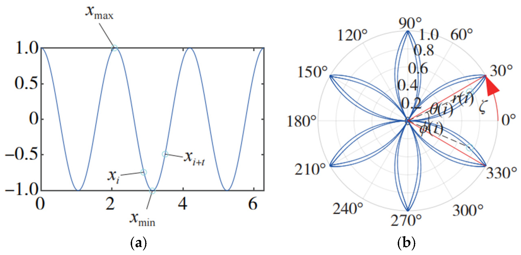
The principle of SDP is illustrated in Figure 2. For a time series signal x , if the value of the i -th sampling point is set to x i , then the value of the sampling point after a time interval of t is x i + t . According to the principle of SDP [25], when the time domain point x i is converted into the polar coordinate space S(r(i), θ(i), φ(i)), the conversion relationship can be expressed by Equation (1):
r i = x i x m i n x m a x x m i n θ i = θ n + x i + t x m i n x m a x x m i n ξ ϕ i = θ n x i + t x m i n x m a x x m i n ξ
where x m i n and x m a x respectively correspond to the minimum value and maximum value of the time domain signal. On the basis of selecting the angle θ n of the n-th mirror symmetry plane as the symmetric axis of the polar coordinate system, a unique fan-shaped lobe diagram can be constructed. θ(i) and φ(i) respectively represent the clockwise and counterclockwise rotation angles along the n-th mirror symmetry plane in the polar coordinate system. With the dynamic changes in magnification factor ξ and time delay factor t, each sampling point of the time-domain signal can be presented in the polar coordinate diagram in a straightforward and accurate manner. Under different parameter settings, each sampling point exhibits a completely different distribution pattern.
In the SDP analysis process, each element of the time series will be converted into a scattered dot pair in the polar coordinate system. Ultimately, two symmetric lobes will gradually take form within a specific angle range [ θ ξ , θ + ξ ], providing a unique and effective way for visualizing signal features, as shown in Figure 2. Here, the angular gain factor ξ plays the role of defining the boundary of lobe angular distribution, while the time delay coefficient t has a considerable impact on the shape of the lobes.

2.3. SDP Parameters Optimization Algorithm

In the process of SDP signal processing, the selection of θ, ξ and t is of crucial importance. Each of these parameters has a significant impact on the presentation of the final image. Specifically, θ determines the number of mirror symmetry planes: as the value of θ increases, the number of mirror symmetry planes will increase. However, the increase in the number of mirror symmetry planes gives rise to image overlapping, which will lead to confusion in image information thus bringing extra difficulty to subsequent analysis. If the value of θ is too small, the symmetry of the generated image will not be prominent enough, making it difficult to give full play to the advantages of the SDP method. ξ affects the angle between the center of mass and the initial line, while t affects the plumpness of the lobes.
The k-th rotation angle of the mirror plane is expressed by Equation (2):
θ k = 360 k m , k = 0,1 , , m 1
where m represents the number of lobes, and k represents the number of symmetric arms in the pattern.
Therefore, it can be concluded that whether different types of images can be distinguished based on SDP images depends heavily on parameters ξ and t. Setting appropriate values for ξ and t can significantly enhance the detailed information in SDP images and highlight the differences between images corresponding to different signals to the maximum extent, making it easier to distinguish images.
In order to select the most suitable parameters, this paper uses the normalized cross-correlation coefficient as a key evaluation indicator for choosing the optimal parameter combination. The cross-correlation coefficient between image matrices A and B from different categories can be calculated by Equation (3):
r A , B = i = 1 M 1 j = 1 M 2 A i j A ¯ i = 1 M 1 j = 1 M 2 B i j B ¯ i = 1 M 1 j = 1 M 2 A i j A ¯ 2 i = 1 M 1 j = 1 M 2 B i j B ¯ 2
where M1 and M2 denote the number of rows and columns of matrices A and B, and A - and B - are the average grayscale values, A - = 1 M 1 M 2 i = 1 M 1 j = 1 M 2 A i j , B - = 1 M 1 M 2 i = 1 M 1 j = 1 M 2 B i j , and the value range of r is between 0 and 1. A large value of r means that the similarity between two images in terms of grayscale features and other aspects is high; a small value of r indicates significant differences between the two images.
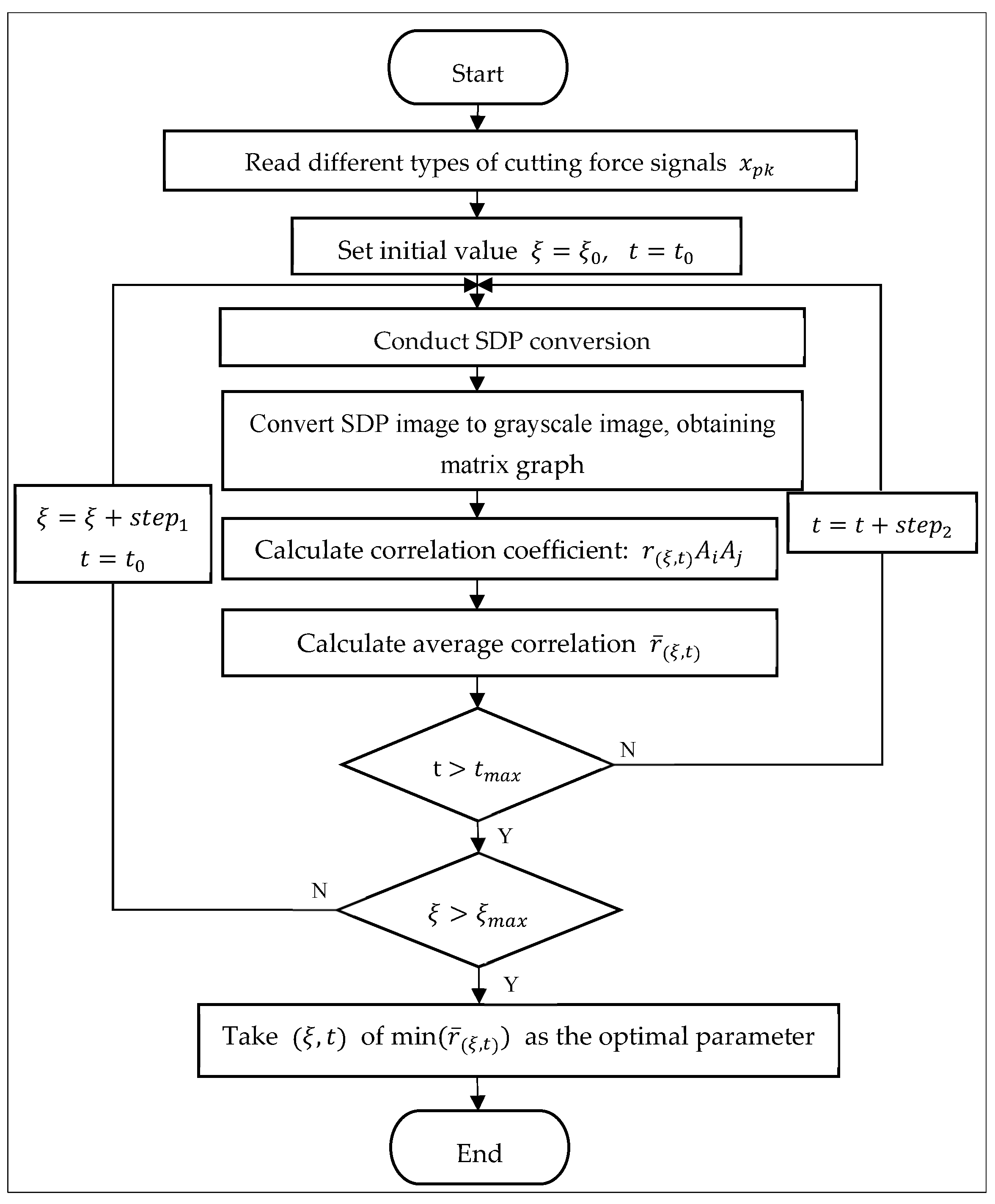
The strategy of SDP parameter optimization and feature map construction is shown in Figure 3.
The procedure mainly includes the following steps:
(1)
Data selection: Select cutting force sample signals {xpk, p = 1, 2, …, P, k = 1, 2, …, K}, p and k represent tool conditions and the sample number of each condition, P and K are the number of tool conditions and the sample size of each condition, respectively;
(2)
Setting parameter range and step size: Set the ranges of ξ and t to ξ0 < ξ < ξmax, t0 < t < tmax, and their respective step sizes are step1 and step2;
(3)
SDP conversion and grayscale image generation: Perform SDP conversion on the cutting force signal xpk based on the parameter set (ξ, t), and convert it into a grayscale image;
(4)
Calculation of cross-correlation coefficient: Select two samples Api and Aqj (p, q = 1, 2, …, P, i, j = 1, 2, …, K, pq) from different categories, and calculate the cross-correlation coefficient r(ξ,t)ApiAqj using Equation (3);
(5)
Determination of optimal parameter: Calculate the average value of the correlation coefficient in the way shown in Equation (4). The values of t and ξ corresponding to the minimum value of the average value are the optimal parameter values.
r ¯ ξ , t = 2 P P 1 K 2 p = 1 P i = 1 K q = 1 , q p P j = 1 K r ξ , t A p i A q j

2.4. ResNet18 Model

Residual network (ResNet) was proposed by He et al. to solve the problems of gradient vanishing and gradient explosion in deep convolutional neural networks, which can occur as the model depth increases [27]. Residual networks are easy to optimize, and accuracy can be improved by increasing the depth. The residual blocks inside a residual network adopt skip connections to mitigate the problems of gradient vanishing and model degradation in deep neural networks caused by increase in depth. Its biggest feature of residual networks is the use of skip connections between network layers, which makes it possible to train deeper networks than before, thus achieving higher accuracy. The residual unit can be expressed by Equation (5):
x l + 1   =   x l   +   F x l , ω l
where x l and x l + 1 respectively represent the model input and output of the l -th layer in the residual network, F is the residual function, and ω l is the network weight f the l -th layer. The F function can be modified according to task needs, F ( x )   =   ω 2 σ ( ω 1 x ) , where σ represents the ReLU activation function whose bias is omitted, w1 and w2 are the network weight f the first and second layers respectively. When F is a layer, the output can be regarded as the result of the input passing through a linear layer once, which is y   =   x   +   ω 1 x , and the stacking layer learns new features after learning the input features. In this way, the model is optimized and updated continuously. Moreover, when the model fits the residual function F(x), the process is much simpler than directly fitting the mapping function H(x) = x, and the change in feature weight is very small after passing through each layer of the network. However, the residual function F(x) and the direct mapping x have completely different variation trends. It is obvious that the output change in F(x) has a greater effect on adjusting weights; therefore, it can achieve better results. The idea of residual is to remove the same main part so as to highlight minor changes.

3. Experiment and Observation

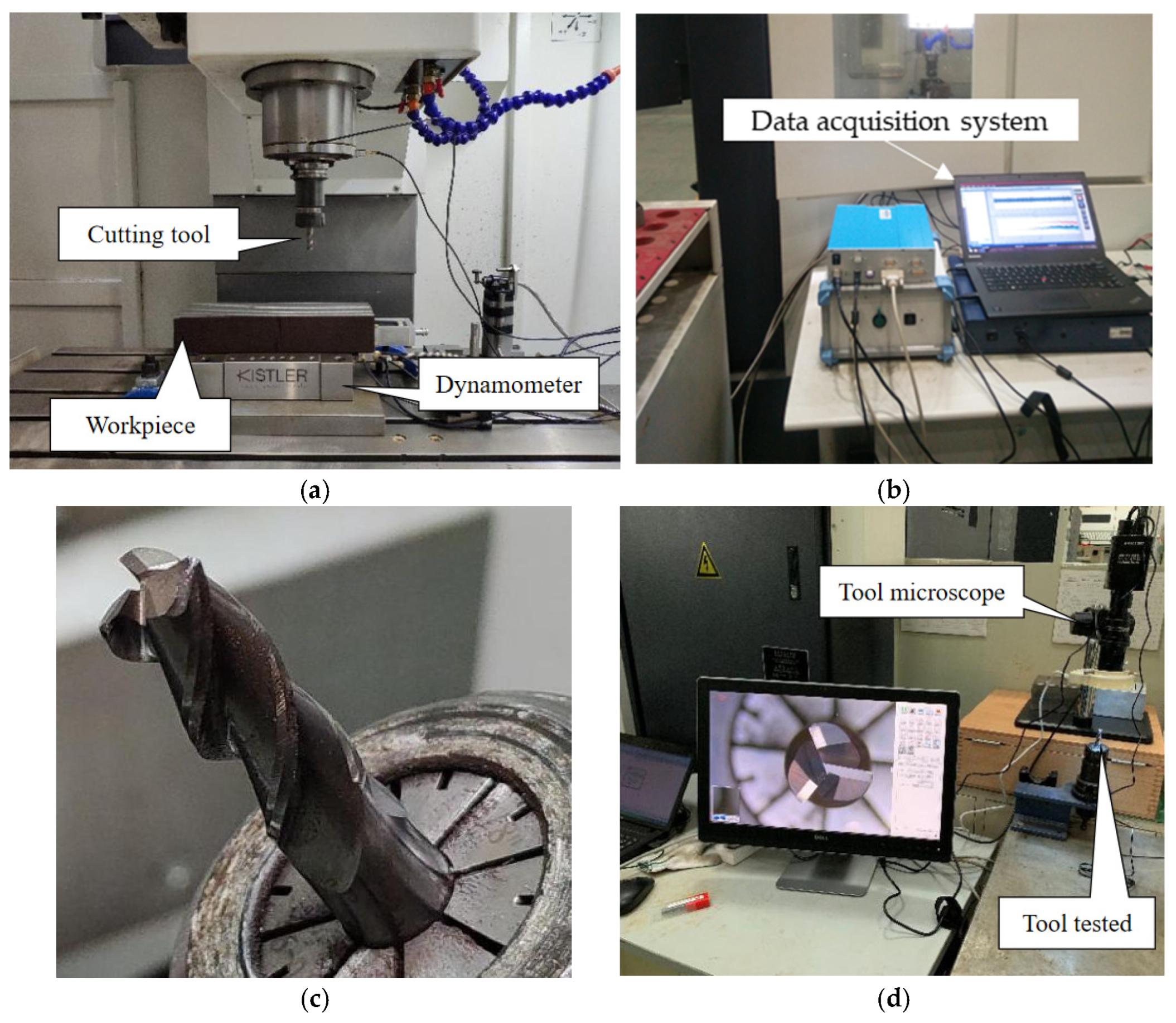
The TCM experimental platform, as shown in Figure 4a, uses the dry milling method to mill workpieces on a vertical machining center (DMTG VDL850A, Dalian Machine Tool Co., Ltd, Dalian, China). The dimensions of the workpiece to be processed are 300 mm × 100 mm × 80 mm, and the material of the workpiece is AISI-1045 (shown in Table 1). A Φ10 mm three-slot straight-shank tungsten steel end mill cutter (Changzhou Pengjin Precision Tools Co., Ltd., Changzhou, China) was selected for the cutting operation in the experiment (as shown in Figure 4c).
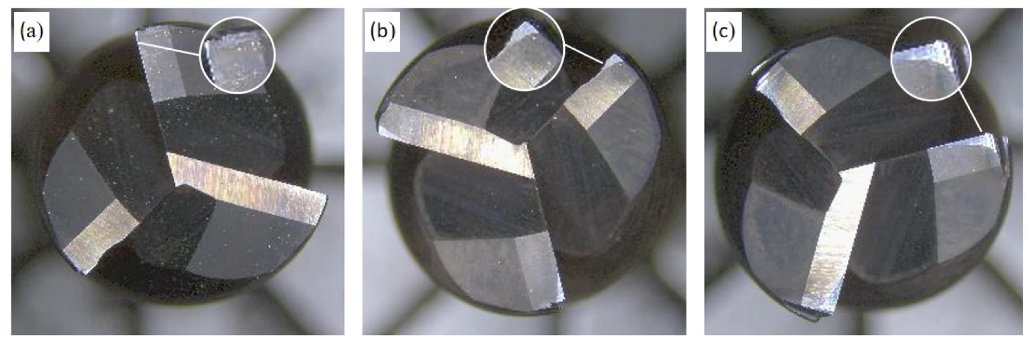
The procedure of the experiment is as follows: a brand new milling cutter is selected to perform milling on the entire surface of the workpiece through forward and reverse milling operations. This complete machining process is defined as a tool cutting state. A Kistler dynamometer (9139AA) is installed between the workpiece and the workbench to measure the cutting force during the cutting process (as shown in Figure 4a). A signal acquisition system is used to collect, amplify, and store cutting force signals (as shown in Figure 4b). Throughout the entire signal acquisition process, the sampling frequency is kept at 12 KHz. After completing each milling stage, the cutting operation is halted, and the end milling cutter is removed. The wear degree of the milling cutter is measured using a tool microscope, and the wear image is recorded (as shown in Figure 4d). Each end milling cutter will be used repeatedly until it becomes unusable. Figure 5 shows the wear images of the first end milling cutter after finishing the first, fifth, and tenth milling stages.
In total, fourteen end milling cutters made of identical materials were used for TCM experiment under different cutting conditions. The cutting parameters are shown in Table 2. In order to assess the actual wear state of each end milling cutter more comprehensively, this paper proposes to use the wear area of the milling cutter end face as the metric for measuring wear degree. Specifically, the wear area of the tooth with the most severe wear among the three teeth of the milling cutter is selected as the wear value of the milling cutter [28]. All the end milling cutters used in the experiment are brand new at the beginning of the experiment. When the wear value of an end milling cutter reaches 0.8 mm2, it will no longer be used in the experiment. After each milling stage is completed, its wear value (maximum wear area) corresponding to this stage is measured. According to the wear trend, the wear degree of the end milling cutter can be divided into five states: initial wear, slight wear, stable wear, sharp wear, and failure, as shown in Table 3.

4. Results and Discussion

4.1. Optimization of SDP Parameters

According to article [29], when the value of t is in the range of 1–10 and the value of ξ is in the range of 10°–50°, the generated SDP images usually have quite good quality. Therefore, ξmax = 50° and tmax = 10, and the step sizes of t and ξ are set to step1 = step2 = 1. According to the strategy of parameter optimization shown in Figure 3, the optimization result is as follows: when the combination of t and ξ is (30°, 1), the correlation coefficient is the smallest to 0.0632.
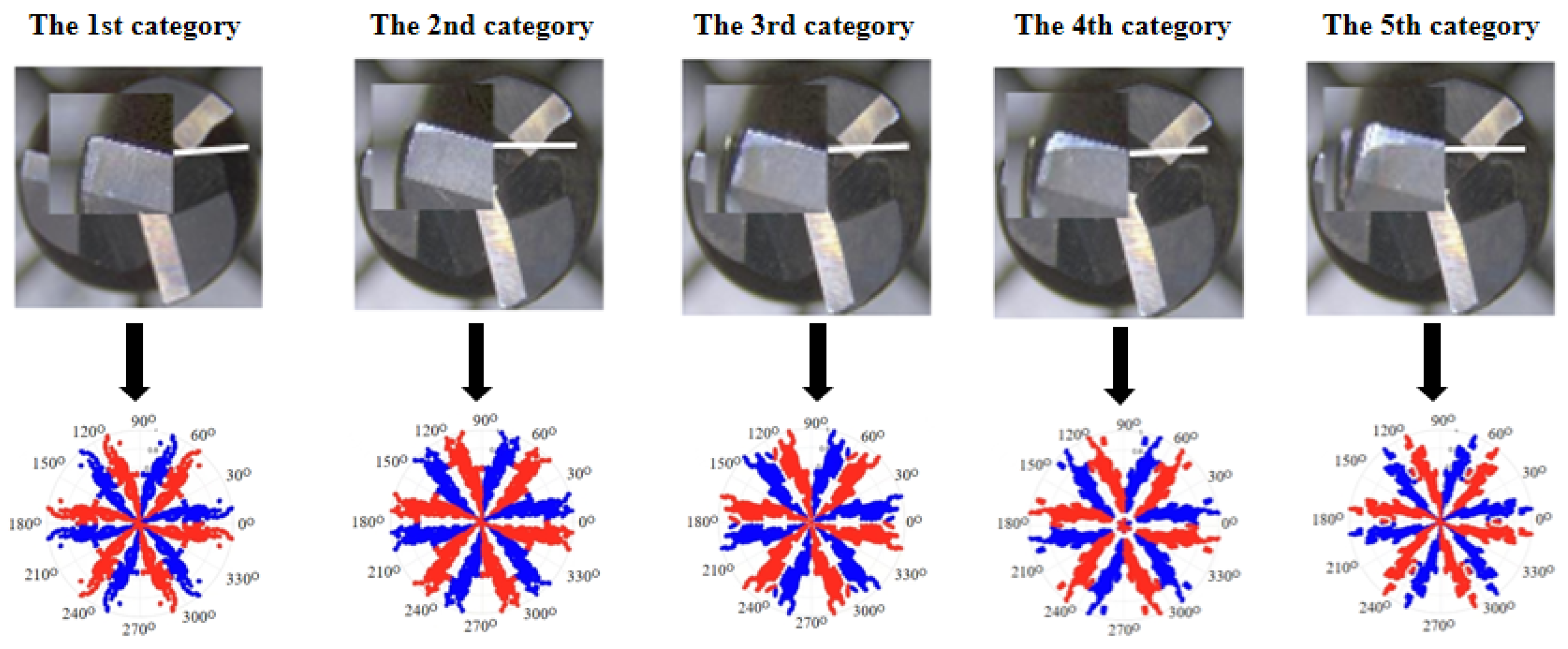
Figure 6 shows the lobe diagrams of parameter-optimized SDP corresponding to different wear states of the first end milling cutter. As can be seen easily from the five types of SDP lobe diagrams, the end milling cutter in question exhibits significantly different patterns under different wear states.

4.2. Comparison of Model Results

SDP conversion was performed based on the results of SDP parameter optimization, with the corner gain factor set to 30°, the time delay factor set to 1, and the window sliding length set to 512. An experimental dataset was constructed, with 600 samples for each tool condition. The dataset was divided into training set, verification set and testing set in a 3:1:1 ratio. For each tool condition, the training set contains 360 samples, the verification set contains 120 samples, and the test set contains 120 samples. In order to test the effectiveness of the proposed method, we selected five popular small sample image classification methods for comparative analysis: STFT ResNet, GAF ResNet, STFT-VGG16, GAF-VGG16, and SDP-VGG16. According to the parameter settings in [30], the window length and step size of STFT are set to 256 and 128 in the STFT-based method, respectively. According to the parameter settings for GAF in [31], the piecewise length of GAF is set to 128. The network structures of the ResNet18 and VGG16 models are shown in Table 4, and detailed information can be found in [27,32].
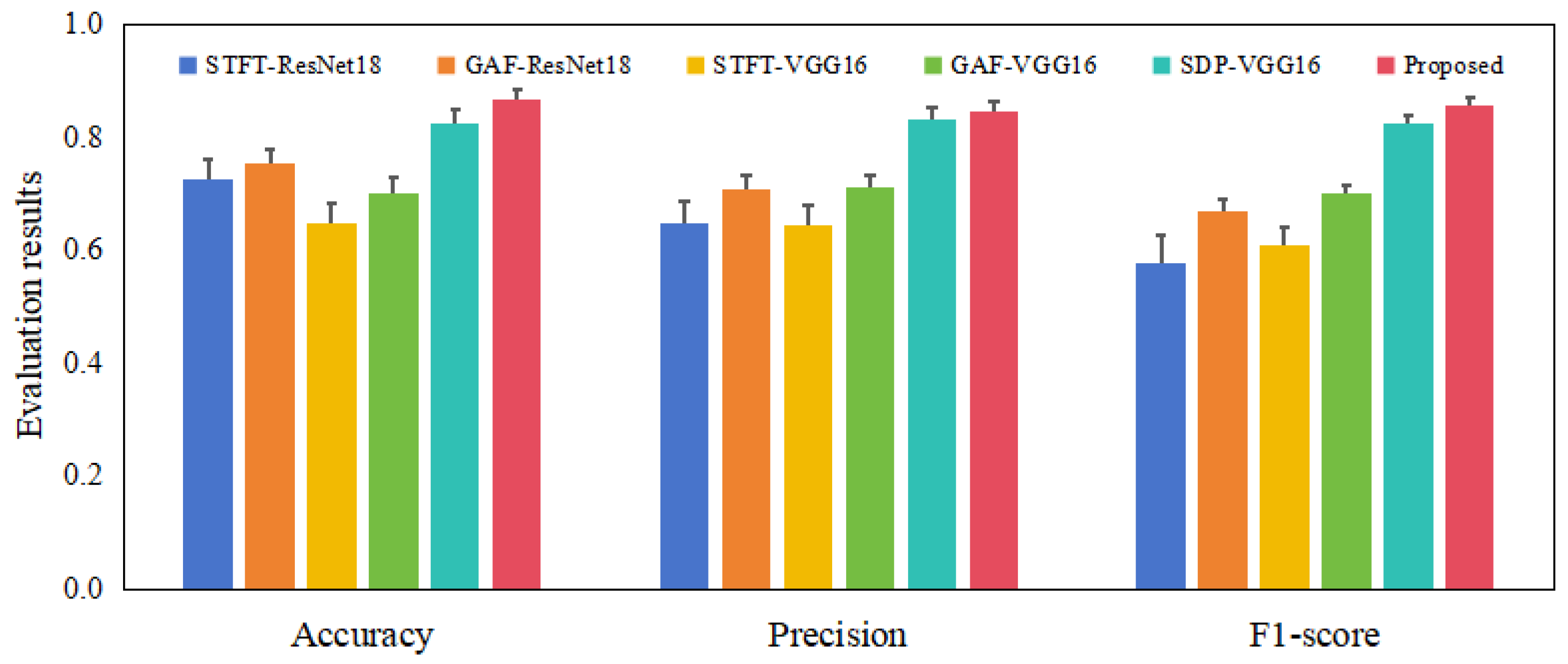
Each method was trained five times, and the obtained average classification accuracy and standard deviations are shown in Figure 7 and Table 5. It can be found from Figure 7 that, among the three signal processing methods, the model trained using the parameter-optimized SDP method has significantly higher testing accuracy than the models trained using the STFT and GAF methods, with a classification accuracy of more than 10% higher. It indicates that compared with STFT and GAF, the SDP method can extract the essential features of the cutting force signals collected in the experiment more effectively. In addition, regardless of which signal processing method is used, the classification accuracy of ResNet18 is higher than that of VGG16, indicating that the proposed method can achieve better classification performance under small samples. From the perspective of error, it can be found from Table 5 that the fluctuation of the proposed SDP-based method is significantly lower than that of the methods based on STFT and GAF, only 46% and 78% of their standard deviations, respectively.
Figure 8 shows the confusion matrix of the proposed method. It can be found that, although the overall classification accuracy of the proposed method is superior to the other methods, there are significant differences in classification accuracy across different conditions. The classification accuracy of the third condition exceeds 90%, but the classification accuracies of the remaining four conditions are only between 84% and 86%.

4.3. Sensitivity Analysis

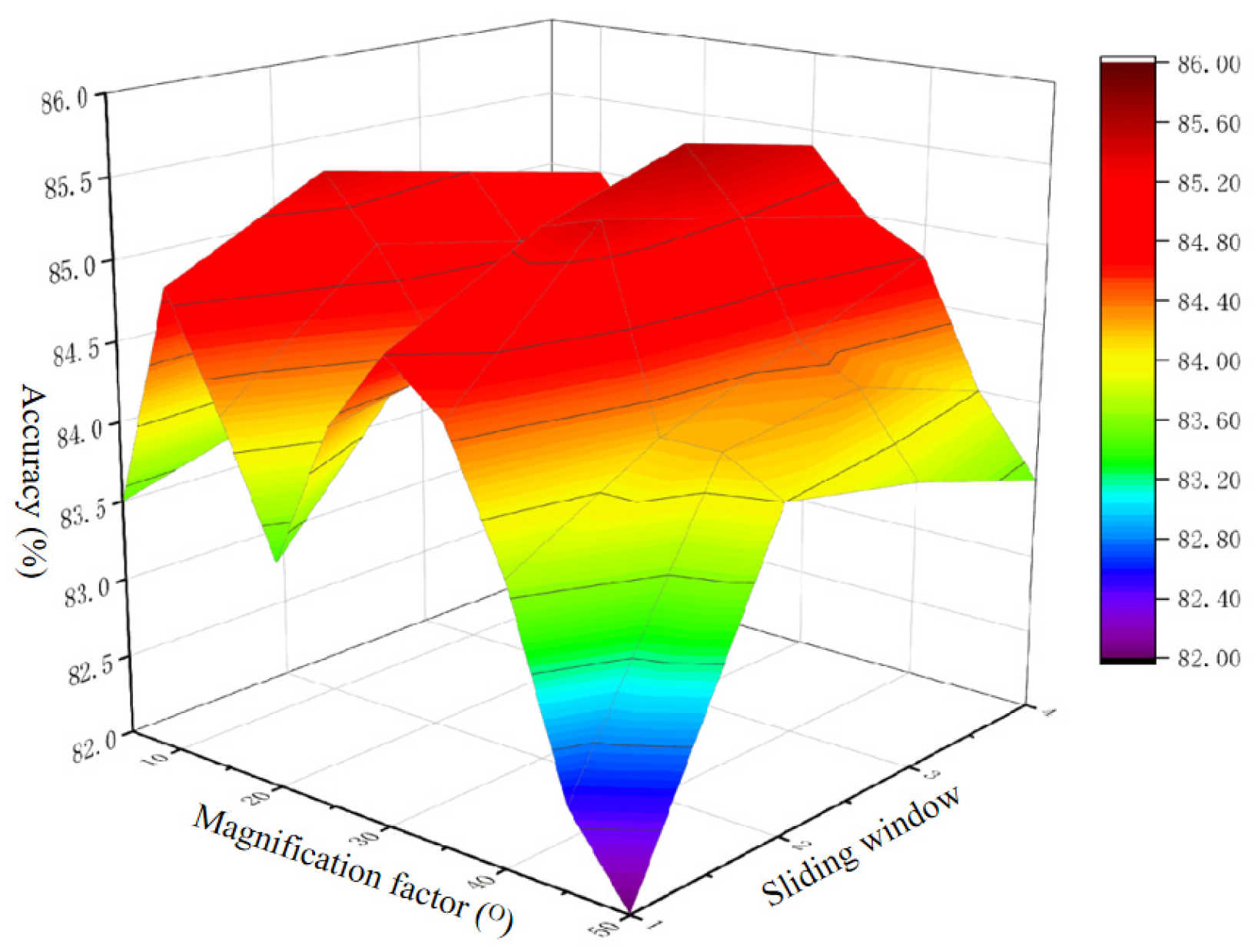
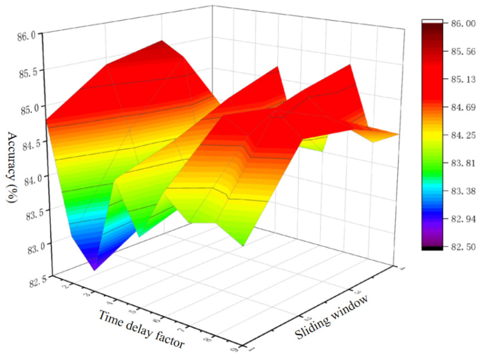
In addition to comparing the impact of the above methods on classification accuracy, we also analyzed the influence of SDP parameters on classification accuracy. Two sensitivity tests were conducted: (1) when the time delay factor t was set to 1, the magnification factor ξ was given a value from 5° to 50°, and the sliding window length was set to 128, 256, 512, and 1024, and the corresponding changes in classification accuracy were observed and recorded. The results are shown in Figure 9. (2) When the magnification factor ξ is set to 30°, the time delay factor t is given a value from 1 to 9, and the sliding window length was set to 128, 256, 512, and 1024, and the corresponding changes in classification accuracy were observed and recorded. The results are shown in Figure 10. For the convenience of observation, the length of the sliding window is represented by numbers 1, 2, 3, and 4 in the figure.
As revealed by comparative analysis, when the magnification factor ξ is 30°, relatively high accuracy can be achieved if the time delay factor t is set to 1 or 2. When t is set to 1, the sliding window has a smaller impact on accuracy, which means better stability. When the time delay factor is fixed to 1, the deviation is relatively large if the magnification factor ξ is in the range of 5°–50°. When the magnification factor is 30° and the sliding window length is 512, the highest accuracy can be achieved. The closer the magnification factor is to 30°, the higher the accuracy, and the smaller the impact of sliding window length on accuracy. Therefore, when the magnification factor ξ of SDP is 30°, the time delay factor t is 1, and the sliding window length is 512, the model has the highest and most stable accuracy.

5. Conclusions

This paper proposes a TCM method based on SDP enhanced ResNet18 to address the problem of low performance in tool wear detection under the condition of a small sample size. The results of a series of experiments conducted on an experimental TCM platform demonstrate that the proposed TCM method is superior to several popular TCM methods.
(1)
The proposed SDP enhanced ResNet 18 method for TCM achieves an improvement of the classification accuracy of over 10% compared to methods based on STFT and GAF.
(2)
The model parameters have a significant impact on the SDP results, and the algorithm proposed to optimize the SDP parameters by minimizing the cross-correlation coefficient can obtain effective model parameters, avoiding the subjective influence on SDP performance.
(3)
In the case of small samples, the TCM classification results based on the Resnet18 model are about 3% higher than those based on the VGG16 model.
The proposed method has shown the potential to improve classification accuracy in small sample situations for TCM, but still cannot achieve good performance. There are several directions worth studying in future research:
(1)
Optimize the SDP algorithm to obtain better feature imaging samples, such as parameter optimization based on evolutionary theory, and obtain richer feature information combining other feature extraction technologies.
(2)
Only 14 tools were conducted in the TCM experiments; leading the repetitive errors are difficult to estimate. Thus, more tool tests will be conducted in the future to eliminate random measurement errors.
(3)
There is a strong correlation between cutting temperature and tool condition. Combining the non-contact advantage of temperature measurement, studying temperature-based TCM methods has great value for industrial applications.

Author Contributions

Conceptualization, X.C. and C.G.; Methodology, G.W. and C.G.; Software, G.W. and H.Z.; Validation, X.C., G.W. and H.Z.; Formal analysis, Y.F.; Investigation, X.C., G.W. and Y.F.; Resources, X.C., G.W. and Y.F.; Data curation, X.C., G.W. and Y.F.; Writing—original draft, X.C. and Y.F.; Writing—review & editing, H.Z. and C.G.; Visualization, X.C. and H.Z.; Supervision, C.G.; Project administration, C.G.; Funding acquisition, C.G. All authors have read and agreed to the published version of the manuscript.

Funding

This work was supported in part by the Research Projects of Zhejiang Provincial Department of Education in China (Grant. Y202354102), in part by the Science and Technology Plan Project of Jiaxing City in China under Grant 2025CGZ057, and in part by the Science and Technology Plan Project of Wenzhou (Grant. G20220006).

Data Availability Statement

The original contributions presented in the study are included in the article, further inquiries can be directed to the corresponding author.

Conflicts of Interest

The authors declare no conflict of interest.

References

  1. Mohanraj, T.; Kirubakaran, E.; Madheswaran, D.; Naren, M.; Dharshan, S.; Ibrahim, M. Review of advances in tool condition monitoring techniques in the milling process. Meas. Sci. Technol. 2024, 35, 092002. [Google Scholar] [CrossRef]
  2. Zhou, Y.; Xue, W. Review of tool condition monitoring methods in milling processes. Int. J. Adv. Manuf. Technol. 2018, 96, 2509–2523. [Google Scholar] [CrossRef]
  3. Kulkarni, N.; Valente, N.; Sabato, A. Time-Inferred Autoencoder: A noise adaptive condition monitoring tool. Mech. Syst. Signal Process. 2023, 204, 110789. [Google Scholar] [CrossRef]
  4. Jing, C.; He, X.; Xu, G.; Li, L.; Yao, Y. Finite Element Modeling Assisted Deep Subdomain Adaptation Method for Tool Condition Monitoring. Processes 2025, 13, 545. [Google Scholar] [CrossRef]
  5. Hei, Z.; Sun, B.; Wang, G.; Lou, Y.; Zhou, Y. Multi-feature spatial distribution alignment enhanced domain adaptive method for tool condition monitoring. Eksploat. I Niezawodn. Maint. Reliab. 2023, 25, 171750. [Google Scholar] [CrossRef]
  6. Zhi, G.; He, D.; Sun, W.; Zhou, Y.; Pan, X.; Gao, C. An edge-labeling graph neural network method for tool wear condition monitoring using wear image with small samples. Meas. Sci. Technol. 2021, 32, 064006. [Google Scholar] [CrossRef]
  7. Mishra, D.; Pattipati, K.; Bollas, G. Gaussian mixture model for tool condition monitoring. J. Manuf. Process. 2024, 131, 1001–1013. [Google Scholar] [CrossRef]
  8. Fu, Y.; Zhong, M.; Huang, J.; Jiang, Y.; Sun, W.; Lou, Y.; Wang, G.; Zhou, Y. Denoising diffusion probabilistic model enhanced tool condition monitoring method under imbalanced conditions. Meas. Sci. Technol. 2024, 36, 015018. [Google Scholar] [CrossRef]
  9. Zhou, Y.; Wang, H.; Wang, G.; Kumar, A.; Sun, W.; Xiang, J. Semi-Supervised Multiscale Permutation Entropy-Enhanced Contrastive Learning for Fault Diagnosis of Rotating Machinery. IEEE Trans. Instrum. Meas. 2023, 72, 3525610. [Google Scholar] [CrossRef]
  10. Zhao, P.; Lin, B.; Zhou, J.; Lv, B.; Li, J.; Zhang, J.; Wang, L.; Sui, T. Review of grinding temperature theory and measurement for the needs of the times: Promoting the development of advanced manufacturing. J. Mater. Process. Technol. 2025, 337, 118744. [Google Scholar] [CrossRef]
  11. Chen, X.; Kong, X.; Yang, M.; Qiang, F.; Zhang, Y.; Cui, X.; Liu, M.; Li, B.; Ma, X.; Li, C. Heat transfer in cutting and grinding processes: Mechanisms, models, and applications. Front. Mech. Eng. 2025, 20, 22. [Google Scholar] [CrossRef]
  12. Kumar, A. Research overview and prospect in condition monitoring of compressors. Expert Syst. Appl. 2025, 277, 127284. [Google Scholar] [CrossRef]
  13. Gao, C.; Nuawi, M.; Wang, J. Tool condition monitoring using I-kaz enhanced kernel extreme learning machine. Eng. Res. Express 2024, 6, 045569. [Google Scholar] [CrossRef]
  14. Yin, H.; Wang, Y.; Sun, W.; Wang, L. Fault diagnosis of hydraulic system based on D-S evidence theory and SVM. Int. J. Hydromechatron. 2024, 7, 1–15. [Google Scholar] [CrossRef]
  15. Zhang, J.; Liu, M.; Deng, W.; Zhang, Z.; Jiang, X.; Liu, G. Research on electro-mechanical actuator fault diagnosis based on ensemble learning method. Int. J. Hydromechatron. 2024, 7, 113–131. [Google Scholar] [CrossRef]
  16. Zhu, Q.; Sun, B.; Zhou, Y.; Sun, W.; Xiang, J. Sample augmentation for intelligent milling tool wear condition monitoring using numerical simulation and generative adversarial network. IEEE Trans. Instrum. Meas. 2021, 70, 3516610. [Google Scholar] [CrossRef]
  17. Zhou, Y.; Sun, B.; Sun, W.; Lei, Z. Tool wear condition monitoring based on a two-layer angle kernel extreme learning machine using sound sensor for milling process. J. Intell. Manuf. 2022, 33, 247–258. [Google Scholar] [CrossRef]
  18. He, X.; Zhong, M.; He, C.; Wu, J.; Yang, H.; Zhao, Z.; Yang, W.; Jing, C.; Li, Y.; Gao, C. A Novel Tool Wear Identification Method Based on a Semi-Supervised LSTM. Lubricants 2025, 13, 72. [Google Scholar] [CrossRef]
  19. Hei, Z.; Yang, H.; Sun, W.; Zhong, M.; Wang, G.; Kumar, A.; Xiang, J.; Zhou, Y. Multiscale conditional adversarial networks based domain-adaptive method for rotating machinery fault diagnosis under variable working conditions. ISA Trans. 2024, 154, 352–370. [Google Scholar] [CrossRef] [PubMed]
  20. Yang, X.; Yuan, R.; Lv, Y.; Li, L.; Song, H. A Novel Multivariate Cutting Force-Based Tool Wear Monitoring Method Using One-Dimensional Convolutional Neural Network. Sensors 2022, 22, 8343. [Google Scholar] [CrossRef]
  21. Cheng, Y.; Xue, J.; Lu, M.; Zhou, S.; Gai, X.; Guan, R. MS-DenseNet-GRU tool wear prediction method based on attention mechanism. Struct. Health Monit. 2025, 24, 517–533. [Google Scholar] [CrossRef]
  22. Dai, L.; Liu, T.; Liu, Z.; Jackson, L.; Goodall, P.; Shen, C.; Mao, L. An Improved Deep Learning Model for Online Tool Condition Monitoring Using Output Power Signals. Shock. Vib. 2020, 2020, 8843314. [Google Scholar] [CrossRef]
  23. Li, S.; Li, M.; Gao, Y. Deep Learning Tool Wear State Identification Method Based on Cutting Force Signal. Sensors 2025, 25, 662. [Google Scholar] [CrossRef] [PubMed]
  24. Sun, Y.; Li, S. Bearing fault diagnosis based on optimal convolution neural network. Measurement 2022, 190, 110702. [Google Scholar] [CrossRef]
  25. Liang, G.; Song, X.; Liao, Z.; Jia, B. Optimal Time Frequency Fusion Symmetrized Dot Pattern Bearing Fault Feature Enhancement and Diagnosis. Sensors 2024, 24, 4186. [Google Scholar] [CrossRef]
  26. Wang, H.; Xu, J.; Gao, Y. New intelligent bearing fault diagnosis method using SDP representation and SE-CNN. IEEE Trans. Instrum. Meas. 2020, 69, 2377–2389. [Google Scholar] [CrossRef]
  27. He, K.; Zhang, X.; Ren, S.; Sun, J. Deep Residual Learning for Image Recognition. In Proceedings of the 2016 IEEE Conference on Computer Vision and Pattern Recognition (CVPR), Las Vegas, NV, USA, 27–30 June 2016. [Google Scholar] [CrossRef]
  28. Zhou, Y.; Zhi, G.; Chen, W.; Qian, Q.; He, D.; Dun, B.; Sun, W. A new tool wear condition monitoring method based on deep learning under small samples. Measurement 2022, 189, 110622. [Google Scholar] [CrossRef]
  29. Zheng, Y.; Niu, L.; Xiong, X.; Qi, H.; Xie, H. Fault diagnosis of CNN bearing cage based on EMD-SDP feature fusion. J. Mech. Electr. Eng. 2021, 38, 81–87. [Google Scholar] [CrossRef]
  30. Wang, J.; Abdullah, S.; Arifin, A.; Singh, S.; Gao, C. A Semi-supervised Fault Diagnosis Method for Rolling Bearing Using TimeFrequency Transform Enhanced Contrastive Learning. Eksploat. I Niezawodn. Maint. Reliab. 2026, 28, 207015. [Google Scholar] [CrossRef]
  31. Wang, H.; Sun, W.; Sun, W.; Ren, Y.; Zhou, Y.; Qian, Q.; Kumar, A. A novel tool condition monitoring based on Gramian angular field and comparative learning. Int. J. Hydromechatron. 2023, 6, 93–107. [Google Scholar] [CrossRef]
  32. Fatima, T.; Soliman, H. Application of VGG16 Transfer Learning for Breast Cancer Detection. Information 2025, 16, 227. [Google Scholar] [CrossRef]
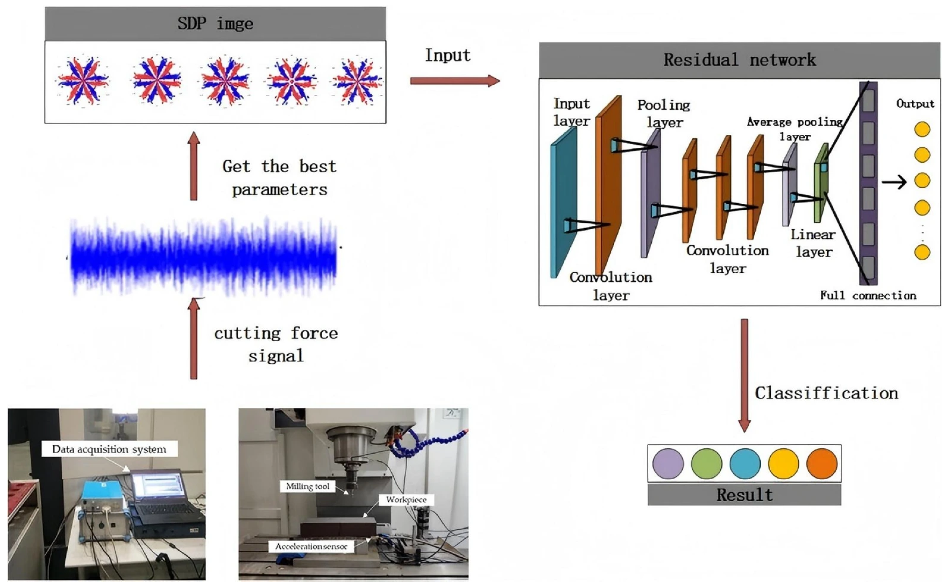
Figure 1. Flow diagram of the proposed method.
Lubricants 13 00503 g001
Figure 2. SDP method theory diagram [26]. (a) Original time-domain signal. (b) SDP lobe diagram.
Lubricants 13 00503 g002
Figure 3. Strategy for SDP parameter optimization and feature map construction.
Lubricants 13 00503 g003
Figure 4. TCM experimental platform. (a) Cutting bench. (b) Data acquisition instrument. (c) Three-slot end milling cutter. (d) Tool microscope.
Lubricants 13 00503 g004
Figure 5. Tool wear images after different milling stages. (a) First cutting stage. (b) Fifth cutting stage. (c) Tenth cutting stage.
Lubricants 13 00503 g005
Figure 6. SDP images of five tool wear conditions.
Lubricants 13 00503 g006
Figure 7. Classification performances of six TCM methods.
Lubricants 13 00503 g007
Figure 8. Confusion matrix of the proposed method.
Lubricants 13 00503 g008
Figure 9. Effect of magnification factor and sliding window length on accuracy.
Lubricants 13 00503 g009
Figure 10. Effect of time delay factor and sliding window length on accuracy.
Lubricants 13 00503 g010
Table 1. Material parameters in J-C model of workpiece material AISI 1045.
A (MPa)B (MPa)CnmTroom (°C)Tmelt (°C)
Value553.1600.80.01340.231201460
Table 2. Cutting parameters in milling experiments.
S/NSpindle Speed (rpm)Cutting Depth (mm)Feed Rate (mm/min)S/NSpindle Speed (rpm)Cutting Depth (mm)Feed Rate (mm/min)
123000.4400825000.5400
223000.5450925000.6450
323000.65001023000.4500
424000.44501123000.6400
524000.55001225000.6500
624000.64001325000.6400
725000.45001425000.4400
Table 3. Classification of tool wear condition and its range.
Tool Category Tool   Wear   Value / mm 2 Tool Wear Condition
1[0, 0.1)Initial wear
2[0.1, 0.3)Slight wear
3[0.3, 0.5)Stable wear
4[0.5, 0.8)Sharp wear
5[0.8, +∞)Failure
Table 4. Network structures of the ResNet18 andVGG16 models.
ComponentResNet18VGG16
Total Layers18 layers16 layers
Convolutional Layers17 layers with 3 × 3 kernel13 (all 3 × 3 kernels)
Fully connected layers1 layer with 1 × 1 kernel3 layers (FC6, FC7, FC8)
Activation FunctionReLU (after each batch norm)ReLU (after every conv/FC)
PoolingAverage pooling before FC layer5 MaxPool layers (2 × 2, stride 2)
Table 5. Classification results of six methods.
STFT-ResNet18GAF-ResNet18STFT-VGG16GAF-VGG16SDP-VGG16Proposed
Accuracy0.725 ± 0.03630.753 ± 0.02350.646 ± 0.03780.701 ± 0.02850.823 ± 0.02400.856 ± 0.0181
Precision0.646 ± 0.03840.707 ± 0.02590.645 ± 0.03370.711 ± 0.01930.832 ± 0.01910.857 ± 0.0156
F1-score0.578 ± 0.04960.669 ± 0.02260.608 ± 0.03120.699 ± 0.01520.817 ± 0.01450.841 ± 0.0143
Disclaimer/Publisher’s Note: The statements, opinions and data contained in all publications are solely those of the individual author(s) and contributor(s) and not of MDPI and/or the editor(s). MDPI and/or the editor(s) disclaim responsibility for any injury to people or property resulting from any ideas, methods, instructions or products referred to in the content.