Measurement Strategies for the Monitoring of the Electric Behavior of Journal Bearings

Abstract

The condition monitoring of machine elements and, more precisely, journal bearings, is beneficial to prevent unnecessary wear and identify critical operating conditions. One method for that is the monitoring of the electric behavior of the bearing by monitoring its capacitance. While the general electric behavior of journal bearings is known, assessments of suitable measurement setups and data analysis methods are usually neglected. This contribution identifies potential measurement setups and analysis methods used in the literature for monitoring rolling-element bearings or journal bearings. These setups and analysis methods are then discussed theoretically and based on measurements of the electric behavior of journal bearings. The findings show that voltage divider setups with AC signals are the most promising solution to monitor the journal bearing electrically. Linear regression algorithms can be used to obtain the amplitude and phase of the measured voltage signal. These values are then used to calculate the impedance and capacitance of the bearing. Lastly, this contribution investigates how existing PCT (percent contact time) analyses need to be altered to improve the precision and robustness of the analysis and allow for the physical interpretation of the measurement results. These findings may be used in the future to predict wear and identify critical operating conditions in journal bearings, such as mixed lubrication.

1. Introduction

Within the context of Industry 4.0, monitoring the condition of systems to provide safety and security and optimize maintenance intervals remains an important goal [1]. For that purpose, suitable sensors and measurement methods have to be identified that can obtain the necessary data. In recent years, the concept of sensory-utilizable machine elements promises to use behavior that is intrinsic to the machine element to generate information [2]. Examples of this are the electric behavior of lubricated contacts in rolling-element bearings [3,4], helical gears [5] and journal bearings [6]. Some research also aims to improve the electric models to be able to predict the electrically induced bearing damage in electric motors and their transmissions, which also requires the measurement of the electric behavior of bearings [7].

Journal bearings are one category of bearing that consist of a bearing shell, the shaft and a lubricant, as can be seen in Figure 1. The main focus of this contribution is hydrodynamic journal bearings. In this type of bearing, the lubrication film is created through the rotation frequency $\omega$ of the shaft and the simultaneous eccentricity e caused by the acting force F. This causes a constriction of the lubrication film down to the minimum lubrication film thickness $h_0$. If the minimum lubrication film thickness is large enough to separate the asperities of the shaft from the asperities of the shell, hydrodynamic lubrication is achieved. Journal bearings are generally used in applications where continuous operation at high rotation speeds are required [8], such as in the energy industry [9,10], aircraft turbines [11] and ship drive trains [12].

Although journal bearings have become increasingly more important due to their high efficiency at high rotation speeds, unexpected failure in potentially safety-critical applications still occurs [13]. Research into the electric behavior of journal bearings could allow the monitoring of these bearings in future to prevent or reduce the amount of unexpected failures; however, research into this topic is limited. This is despite the fact that few other condition-monitoring solutions for these bearings exist. As Koetz et al. showed, the monitoring of the electric behavior of a hydrodynamic journal bearing allows the detection of mixed lubrication [6], which is a critical failure mode of journal bearings [13].

However, multiple approaches and concepts exist which allow the measurement of the electric behavior of machine elements and specifically journal bearings. Contributions to this research topic rarely discuss different measurement concepts and setups. Therefore, this contribution aims to discuss different measurement approaches with regard to the electric circuit setup, the electric signal type and the analysis method. Furthermore, the analysis methods are discussed with regard to their suitability to interpret the measurement results obtained. The aim of this is to present the advantages and disadvantages of different measurement and interpretation approaches and identify one approach that maximizes the information generated through the measurement of the electric behavior of journal bearings. The discussion is limited to mixed and hydrodynamic lubrication regimes as those are technically relevant for the electric monitoring of journal bearings.

In line with the aim of this study, the following research questions will be answered:

• RQ1: Which electric circuit setups and electric signal types can be used to measure the electric behavior of journal bearings for mixed and hydrodynamic lubrication robustly?
• RQ2: Which analysis methods can most reliably be used to quantify the electric behavior of the journal bearing bearing based on the measurement signals?
• RQ3: How can the data analysis method be optimized to improve the physical interpretation of the measurement results and allow for the development of wear models in future?

2. Materials and Methods

In this section, the state of research is discussed. Thereafter, the basics for this contribution are outlined such as the electric behavior of journal bearings, measurement setups from the literature, the test bench that was used to generate the measurement results for this contribution and data analysis methods.

2.1. State of Research

To investigate the state of research on journal bearing impedance measurement, a literature review was performed based on the PRISMA 2020 statement [14]. The search was performed using the database “Web of Science” with the search string “ALL = ((capacitance AND bearing) OR (impedance AND bearing)) AND ALL = (measurement) AND (ALL = ((electric) OR (electrical)))”, yielding 392 results.

A title screening of the results yielded 324 results which were not relevant to bearings and mechanical engineering. A total of 28 results specifically dealt with the electric behavior of rolling elements or rolling-element bearings. A further 36 results mentioned bearings in general; however, upon reviewing the abstracts and the results, it became clear that they also specifically dealt with rolling-element bearings in electric motor applications. Only two contributions could be identified that directly dealt with journal bearings. Cui et al. dealt with the capacitance measurement of lubrication film by applying a external capacitive distance sensor on a shaft [15]. This is not the aim of this current study, as the overarching goal of the research presented here lies in using the intrinsic capacitive behavior of journal bearings. Koetz et al. dealt with the electric behavior of journal bearings and showed that the measurement can be used to identify the lubrication condition of the bearing in detail [6].

From the results concerning rolling-element bearings, some conclusions can be drawn with regard to the measurement setup used. Clarke et al. use the measured voltage signals directly to monitor the electric behavior of rolling-element bearings [16]. This works in principle; however, the voltage is a result of the electric properties of the bearing and is dependent on the measurement setup. Therefore, for the analysis of the electric behavior, this is not deemed sufficient and a calculation of the electric properties such as capacitance or impedance should be performed to be independent of the measurement setup.

One method found in the literature is the use of the charging curve of the bearing under DC voltage, as used by Wittek and others [7,17,18,19]. Other measurement setups used include voltage dividers, such those used by Martin et al. and others [6,20,21]. Sometimes, this is also referred to as shunt measurement [22] but it is the same working principle. An alternative circuit setup is an AC Wheatstone bridge, as used by Puchtler et al. [3]. Some publications also specifically used an impedance analysis device, such as in Hausmann et al.’s work [5]; however, due to the fact that the device can be considered a black box, this measurement setup is not discussed here.

Apart from in the work of Puchtler et al., the measurement setup is rarely a subject of discussion but rather one setup is used that works sufficiently for the specific aim of the publication. Therefore, this contribution aims to take the measurement concepts from these publications and discuss their suitability to monitor the electric behavior of journal bearings.

2.2. Electric Behavior of Journal Bearings

The electric behavior of tribological contacts and more precisely journal bearings has been known for decades, particularly through the work of Prashad [23,24,25,26]. In his work, the journal bearing is modeled according to a parallel eccentric cylindrical capacitor in a fully flooded hydrodynamic contact. Bittner and Kluth showed that alternatively, the bearing can be modeled as a plate capacitor [27]. In recent years, Furtmann extended the work on the journal bearing capacitance to include the tilting of the shaft [18].

Capacitive components are represented by their electric capacitance C, with two electrically conductive surfaces as electrodes, which are separated by a dielectric material. The capacitance C is then dependent on the overlapping area between the two plates, the distance and the permittivity of the dielectric material. The measurement of the capacitance C can be performed by utilizing the electric properties of a capacitance when loaded with AC voltage or DC voltage [28,29].

2.2.1. DC Voltage Behavior

When a capacitance is subjected to a DC voltage, a charging curve can be measured. This charging curve is determined by the time constant $\tau$, which can be calculated using Equation (1), with the charging resistance R and the capacitance of the capacitor C. It is known that a capacitor reaches $62\%$ of its charge after $\tau$. Therefore, the time taken until $62\%$ of its charge can be measured and used to calculate the capacitance C [30]. A visualization of such a signal is included in Figure 2 (blue line), using a voltage signal that discharges with a virtual resistance of $0\Omega$ at $0.05$ s when a discharge is triggered. In reality, the discharge resistance is never $0\Omega$, but for the capacitance measurement, this is not important. The charge of the capacitor starting at $0.1$ s is what is measured. The capacitor charges over a known resistance with an observed time constant $\tau$ of $0.01$ s. Using the known resistance R and the measured time constant $\tau$, the capacitance C can be calculated using Equation (1).

$$\tau =R·C$$

(1)

2.2.2. AC Voltage Behavior

When capacitances are subjected to AC signals, they act as a complex resistance. This resistance is called impedance Z in AC circuits and can be depicted as a complex number according to Equation (2) [28]. This equation uses the resistance of the circuit R and the capacitive reactance of the capacitor $X_C$.

$$Z=R+j{X}_C$$

(2)

This impedance can also be depicted in the complex plane according to Figure 3. The phase angle $\phi$ determines the phase offset between the measured voltage signal and the reference voltage signal. The reference is usually taken from an ohmic resistor which per definition has a phase of $0^{\circ }$. Consequently, the phase shift $\phi$ of a serial or parallel connection depends on the ratio between the resistance R of the resistor and the reactance $X_C$ of the capacitor. A tribological contact such as a journal bearing is generally modeled as a parallel connection between the resistive behavior of the lubricant and the capacitive behavior between the bearing shell and the shaft. By measuring the apparent impedance of the bearing Z, the reactance $X_C$ and then the capacitance C can be calculated.

One effect observed especially in rolling-element bearings is the electric breakdown of the lubricant, which discharges the capacitor without direct contact [31]. The dielectric strength of mineral oils can be found in the literature as being somewhere between 5 kV/mm and 30 kV/mm [32]. In the case of this study, the maximum voltage applied is 2 V. It can be assumed that the breakdown will occur at the minimum lubrication film thickness around the circumference of the bearing. A simple estimation according to Equation (3) can be used with the critical voltage $V_{crit}$ and the dielectric strength of the mineral oil $E_{crit}$. Assuming a voltage $V_{crit}$ of 2 V and a dielectric strength $E_{crit}$ of 5 kV/mm, the breakdown would occur at a minimum lubrication thickness of $0.4\mathsf{\mu }$m [31].

Journal bearings have significantly greater lubrication film thicknesses than rolling-element bearings. Since a breakdown would occur at a lubrication film thickness of at least $0.4\mathsf{\mu }$m and typical lubrication film thicknesses for journal bearings are generally bigger than that by a factor of 10 or more, the electric breakdown of the lubricant can be neglected for the purpose of this contribution.

$$Vcrit=E_{crit}·h_{crit}$$

(3)

2.3. Test Bench

The test bench for this contribution consists of two rolling element support bearings with the journal bearing housing between them, as depicted in Figure 4. Test bench parameters and measurement parameters are depicted in

Table 1. Overview of test bench parameters.

Name	Value
Shell diameter	35 $\mathrm{m}$$\mathrm{m}$
Shell thickness	30 $\mathrm{m}$$\mathrm{m}$
Temperature	30 °C
Maximum rotation rate	3000 $\mathrm{rpm}$
Maximum force y axis	2000 $\mathrm{N}$
Maximum force z axis	2000 $\mathrm{N}$
Bearing play	100 $\mu$$\mathrm{m}$
Electric voltage amplitude	2 $\mathrm{V}$
Electric signal frequency	10 $\mathrm{k}$$\mathrm{Hz}$

. The journal bearing housing is free-swinging and only supported by the bearing. One horizontal (y-axis) and one vertical (z-axis) displacement mechanism can be used to apply a load on the bearing housing via disc springs. The mechanisms additionally allow a rotation via belt drives which can be used to set up specific tilt angles of the housing. The tilt angle is measured using eddy current sensors. In this contribution, these are only used to ensure a parallel shaft. The oil used for this contribution is a HLP 46 oil manufactured by Mannol.

The shaft of the test bench is driven by an electric motor that is connected via a V-belt which prevents the leaking of currents from the motor onto the shaft. The shaft is contacted electrically via a friction contact consisting of graphite. It allows the transmission of electric signals. The second contact is via the journal bearing housing. The resulting electric circuit is depicted in Figure 5 and is explained in Section 2.4.

2.4. Electric Measurement Setup

The circuit used in this contribution utilizes a shunt measurement setup. In a shunt measurement, the voltage drop over the bearing $V_B$ and over the known reference resistor $V_R$ is measured. The reference resistor is an ohmic resistor with a known resistance, although an impedance would also be possible as long as the value of the impedance was known. The reference resistance used in this contribution is an ohmic resistor with a resistance of $1500\Omega$. With the known resistance, the bearing impedance is $Z_B$ calculated using Equation (4). This measurement setup was described by Martin et al. [20].

$${\displaystyle \frac{Z_{\mathrm{B}}}{R}}={\displaystyle \frac{V_{\mathrm{B}}}{V_{\mathrm{R}}}}$$

(4)

It is important to consider the value of the known resistance R as it has to be chosen to be within the range of values of the impedance to be measured to optimize the accuracy of the measurement [28]. This is problematic when measuring in all lubrication conditions as the bearing impedance can range from $0\Omega$ in boundary lubrication up to a virtually infinite impedance at low electric frequencies and with thick lubrication films.

It should be added that the measurement setup presented so far is already a simplification. The more precise model of the setup is depicted in Figure 6. In this Figure, the known resistance is depicted using the resistance $R_{ref}$ and the inductance $L_{ref}$. The inductance of the resistance leads to a positive phase shift which affects the measurement results of the first oscilloscope measurement; however, at the measurement frequency used in this contribution, the inductance creates a phase shift of less than $1^{\circ }$. Therefore, this inductance can be neglected and only needs to be considered at higher electric frequencies.

A more relevant disturbance when measuring the electric behavior of the lubrication film is the resistive behavior of the lubricant $R_{oil}$. This depends on the oil, the surface area and the lubricaiton film thickness. In practice, machine oil has specific resistances $\rho$ of ${10}^8\Omega ·$m [33]. The surface area $A_{oil}$ of the bearing shell used in this contribution is about $3·{10}^{-3}$ m², with lubrication film thicknesses $h_{min}$ in the region of ${10}^{-5}$ m (as observed in tests and calculated according to DIN 31652 [34]). With these values, Equation (5) shows the resulting oil resistance $R_{oil}$ to be in the region of ${10}^5\Omega$. Since the capacitive reactance $X_C$ caused by the capacitance of the bearing $C_{oil}$ reaches maximum values of 12 k$\Omega$, the resistance of the oil is magnitudes greater and therefore can be neglected in this contribution. This can also be seen in the phase angle in the Results section (e.g., Figure 7b), which reaches values of $-{88}^{\circ }$ during temporary hydrodynamic lubrication. If the resistance was relevant, it would result in significant deviations of the phase angle towards $0^{\circ }$. It should be noted that this simplification is valid for this circuit setup within the observed operating range of the specific bearing used here. If the bearing capacitance changes significantly from the capacitance range of this contribution, the resistance of the oil cannot be neglected. In that case, the electric circuit model in Figure 6 needs to be used to calculate the resistance of the oil $R_{oil}$ and the capacitance of the bearing $C_{oil}$.

$$R_{oil}=\rho ·{\displaystyle \frac{h_{min}}{A_{oil}}}$$

(5)

Similarly, the resistance and the capacitance of the measurement equipment need to be considered. The internal resistance of the picoscope 4444 used in this contribution is 1 M$\Omega$ per channel [35]. Therefore, it is not relevant here, similarly to the resistance of the oil. The capacitance of the measurement equipment is 12 pF [35]. With a maximum capacitive reactance of the oil of 12 k$\Omega$ at 10 kHz (as observed during measurements), the capacitance of the bearing can be calculated as 1.3 nF. Since capacitances in parallel circuits are cumulative, the measurement equipment causes an increase in the observed capacitance of 12 pF and therefore of less than $1\%$. Consequently, in the measurement setup used in this contribution, the measurement equipment can also be neglected.

An alternative measurement setup was published by Puchtler et al., who used an AC bridge. In the AC bridge, the resistors are replaced with capacitors [3]. The main advantage of this setup is that it is robust against environmental influences such as temperature deviations and electromagnetic fields [29]. Both the AC bridge and the shunt measurement have to be balanced for the expected capacitance of the bearing. The measurements taken for this measurement are limited to the shunt measurement setup for the reasons that will be discussed in Section 3.1.

2.5. Data Analysis Methods

The analysis of the DC signal does not require additional signal processing steps for the calculation of the electric behavior. The accuracy of the results may be improved through filtering; however, that is optional. The AC or offset AC signal (see Figure 2), however, need to be analyzed before calculations can be made. For that purpose, a Fast Fourier Transform (FFT) can be used, or a linear regression algorithm, which will be explained in the following.

2.5.1. FFT

The FFT is a common algorithm in signal processing that allows a user to retrieve the phase and the amplitude of a signal. This is necessary as the capacitive electric effects cause a phase shift in the voltage signals as well as a change in amplitude. The signal to be analyzed is usually divided into multiple time windows and the FFT is performed for each window [36]. Since in this contribution, the frequency of the electric signal is known as 10 kHz, the amplitude and phase that the FFT calculates at 10 kHz can be interpreted as the real amplitude and phase of the electric signal.

According to He and Feng, multiple errors may occur in the calculation of the FFT which need to be avoided. Spectral leakage may occur when the signal frequency of the electric signal is not a multiple of the frequency of windows [36]. The Fence Effect also reduces the accuracy of a FFT analysis [36]. Based on the finite number of measurement points in each window, the frequency vector of the FFT also has a limited number of frequencies. The signal frequency to be analyzed, e.g., 10 kHz, has to coincide with one of the entries of the frequency vector for accurate results [36].

A practical example of the problems caused by the fence effect in this application is shown in the following section. The length of a window of the signal is of interest when detecting mixed lubrication; so, ideally, each time window is as short as possible to allow the detection of individual metallic contacts during mixed lubrication. But, the length of a window determines the number of measurement points inside each window. The frequencies to be analyzed in an FFT also contain as many frequencies as there are measurement points in a window. The frequency vector is defined according to Equation (6), with the number of measurement points per window $N_w$, the overall sampling frequency $F_s$ and the length of a window in seconds T. The product of the sampling frequency $F_s$ and the length of a window T results in the number of measurement points per window $N_w$. The smallest non-zero entry of the frequency vector is $1/T$. The frequency vector represents the frequency resolution (also size of a frequency bin) of the analysis which is not influenced by the measurement frequency but only by the length of a window.

$$\overrightarrow{f_{FFT}}=\left(\begin{array}{c}0\\ 1\\ 2\\ N_w-1\end{array}\right)·{\displaystyle \frac{F_s}{F_{s}T}}$$

(6)

Assuming an electric signal frequency of 10 kHz, the time window length has to be at least ${10}^{-4}$ s long to ensure that the smallest entry of the frequency vector is at least the electric frequency. In that case, a metallic contact during mixed lubrication has to last at least 0.1 ms in order to be clearly identified as metallic contact in the FFT signal. However, the actual length of a contact is expected to be significantly shorter. This limits the applicability of the FFT analysis for tribological problems.

2.5.2. Regression Analysis

One alternative to the FFT analysis is a regression analysis. In this case, the relationship between the frequency resolution and window length no longer applies. Since the signal frequency is known, in theory, the regression model requires only a fit of amplitude and phase of the signal. A division into windows is again useful to improve the time resolution of the measurement. However, it is not clear how long a window has to be in order to have a sufficient number of data points in each window.

A least squares method may be applied to identify the best match of amplitude and phase of the sine curve to be matched to the data points [37]. It has to be considered that the minimum residual of the calculated regression model can be a local minimum [38]. This has to be avoided by the algorithm. Another aspect to be considered is the influence of individual contacts between bearing and shaft, which reduce the bearing voltage significantly for a short period of time. These reductions in voltage will have a significant influence on the regression model, as the errors between regression model and measured data are squared [39].

The algorithm used in this study assumes that the measurement signal is described according to Equation (7), with the known signal frequency $\omega$ and the unknown amplitude $\widehat{x}$ and phase offset $\phi$. By using trigonometric identities, Equation (7) can be written as Equation (8). This allows the use of linear regression as opposed to an iterative regression algorithm, which would be necessary when using Equation (7) directly. After solving the linear regression problem, the overall amplitude $\widehat{x}$ and the phase shift $\phi$ can be calculated using Equations (9) and (10) [40].

$$\begin{array}{c}\hfill y=\widehat{x}·sin(\omega ·t+\phi )\end{array}$$

(7)

$$\begin{array}{c}\hfill y=\widehat{x_c}·cos(\omega ·t)+\widehat{x_s}·sin(\omega ·t)\end{array}$$

(8)

$$\begin{array}{c}\hfill \widehat{x}=\sqrt{{\widehat{x_c}}^2+{\widehat{x_s}}^2}\end{array}$$

(9)

$$\begin{array}{c}\hfill \phi =arctan\left({\displaystyle \frac{\widehat{x_c}}{\widehat{x_s}}}\right)\end{array}$$

(10)

2.5.3. PCT

Hemskeerk et al. introduced the concept of the percent contact time (PCT) when monitoring rolling-element bearings. They used DC voltage which was monitored to detect individual electric contacts. The combined time of all contact was then measured and expressed using the percentage of time in which the bearing voltage would drop to zero [21]. This works well for DC voltage monitoring; however, if AC voltages are used, then the concept of the PCT becomes ambiguous. The AC voltage cannot be used to identify contact times easily as the signal passes through 0 V twice in every period. Additionally, when the data analysis method is used to calculate the phase $\phi$ of the capacitive impedance, it shows values between ${10}^{\circ }$ and $-{80}^{\circ }$. It can be assumed that the only physical phase angles in the circuit are $0^{\circ }$ for boundary lubrication and close to $-{90}^{\circ }$ for hydrodynamic lubrication [6]. Every other result is caused by an averaging behavior of the FFT, e.g., $-{45}^{\circ }$ corresponds to a ratio of metallic contact and hydrodynamic lubrication within a time window. Hausmann et al. introduced a method that allows the use of the PCT value for AC voltages despite the limited time resolution and the ambiguity of the phase angle by assuming an averaging behavior of the data analysis method. The PCT can consequently be calculated according to Equation (11) using the phase angle $\phi$ [5].

$$PCT=\{\begin{array}{cc}NA& \mathrm{if}\phi <-{90}^{\circ }\\ 1+{\displaystyle \frac{\phi }{{90}^{\circ }}}& \mathrm{if}-{90}^{\circ }\le \phi \le 0^{\circ }\\ NA& \mathrm{if}\phi >0^{\circ }\end{array}$$

(11)

3. Results

In the following section, the answers to the initial research questions will be given. The first section focuses on the measurement setup and a signal type according to RQ1. The setup is then chosen as a prerequisite to discuss the following research questions of the data analysis method (RQ2) and how to improve the data analysis method to allow for a more accurate interpretation of the results obtained (RQ3).

3.1. Measurement Setup and Signal Type

As discussed in Section 2, the capacitive behavior of bearings can generally be measured using DC voltage signals and AC voltage signals. When DC voltages are applied, the charging curve can be measured and the capacitance calculated through Equation (1).

For that measurement setup, it is necessary to ensure a constant capacitance for the duration of $\tau$. However, this cannot be assumed for tribological systems as individual metallic contacts may occur during this time frame. Additionally, small changes in lubrication film thickness can cause significant changes in capacitance [6], thus reducing the accuracy of this approach.

In practice, this means that the automated analysis of these measurements has to recognize the initiation of a charging curve (e.g., immediately after a metallic contact has occurred). The determination of the exact point in time is difficult as background noise will affect the measured signal, leading to erroneous readings. After the determination of this point, the algorithm has to measure the time until $62\%$ of the charge is reached and ensure that no additional metallic contact occurs during this time. If there is additional metallic contact, the measured time has to be reset and start again. For a human operator, the analysis of a single metallic contact and measurement of $\tau$ is easy; however, the automation of such an algorithm is more complex in systems with transient behavior.

One advantage of the DC measurement is the simple observation of individual metallic contacts, as performed by Hemskeerk et al. [21] and described in Section 2.5.3. This approach only allows the detection of metallic contacts in mixed lubrication but it does not allow a measurement of the lubrication film thickness. However, it is beneficial to measure the lubrication film thickness because this information can be used to determine how much additional load the bearing can support before operating in potentially harmful mixed lubrication. Therefore, for practical purposes, the DC signal is not considered further for the measurement of the electric behavior of journal bearings.

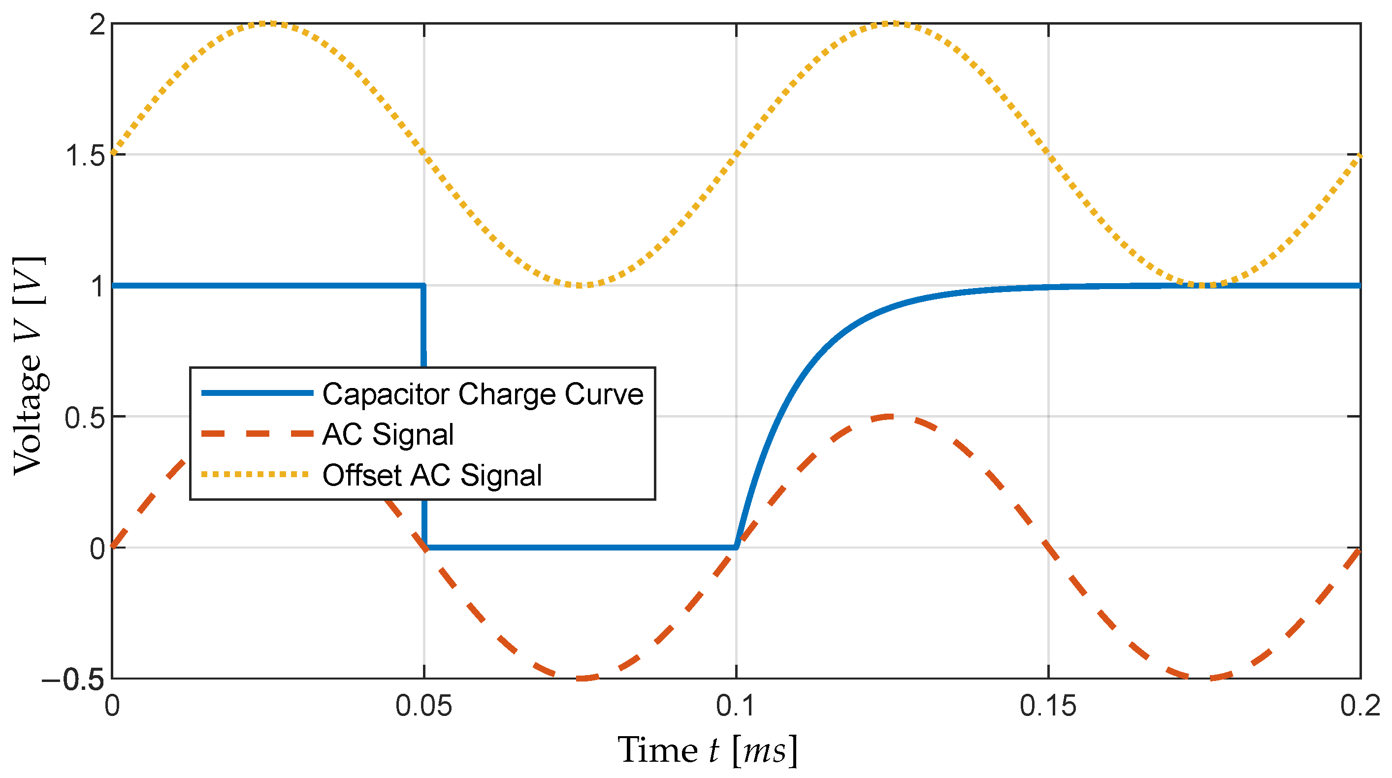
When using AC signals, a simple PCT analysis cannot easily be made as these signals reach 0 V at least twice per period. An automated analysis of contact times is therefore difficult. They also require additional signal analysis methods, as discussed in Section 2.5. However, the advantage of these signal is the long duration which means that periodically repeating dynamic effects (e.g., the roundness deviations of a shaft) can be compensated by averaging the measurement. Therefore, this signal can be considered to be more robust and automated analysis is possible, as will be discussed in Section 3.2.

One last signal type that in theory offers the benefits of both signals is an offset AC signal, as depicted for visualization in Figure 2. In this signal, the AC signal is superimposed with a constant DC signal. If the DC part of the offset signal is sufficiently high, the signal no longer reaches 0 V unless metallic contacts occur. Therefore, the individual contacts can be identified by an algorithm and the data analysis methods mentioned in Section 2.5 can still be used. The choice between an AC signal and an offset AC signal is discussed further in Section 3.3.

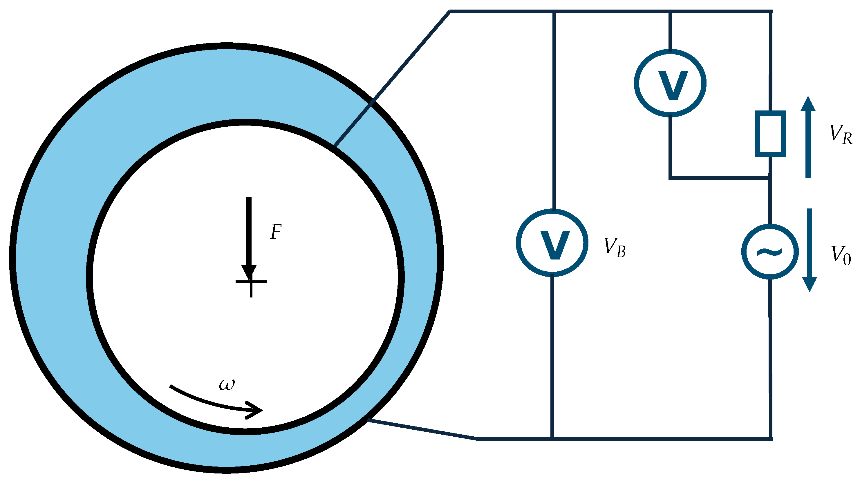
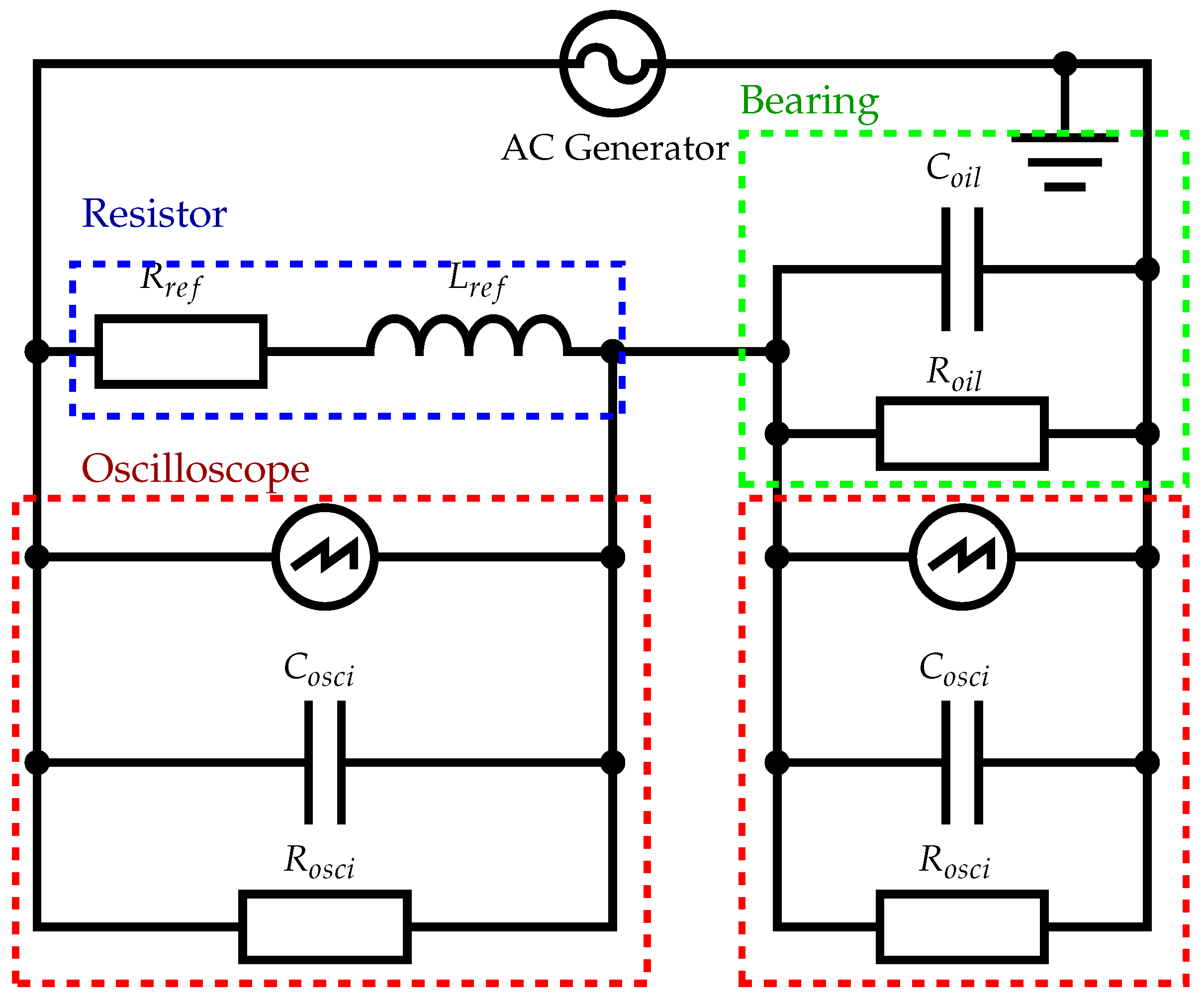
When using AC signals or offset AC signals, a voltage divider-based setup or an AC measurement bridge are both possible measurement setups, as discussed in Section 2.4. The main advantage of the measurement bridge is its robustness against environmental factors such as temperature deviations and the influence of electric fields [3]. Setups based on a voltage divider, however, can easily be modified and adapted to changes in bearing impedance. For the best accuracy, the reference resistance needs to be within the range of magnitudes of the bearing impedance [16]. Since the test bench for this contribution is placed within a controlled environment, the simpler voltage divider setup is used as this setup can be more easily adapted to the fluctuating bearing impedance in different lubrication conditions [3].

3.2. Data Analysis Method

In general, FFT and linear regressions can be used to extract phase and amplitude from a sine signal. In the context of this contribution, the FFT is used as a filtering mechanism to identify known signal frequency from voltage signals. Since the FFT is then no longer a superposition of multiple sine signals but only one sine signal, the FFT and the linear regression yield the same calculation result apart from numerical errors with relative errors between both algorithms of ${10}^{-15}$. Even artificially introduced random noise influences the calculation results of both algorithms equally.

This is the case as long as the FFT calculation is not affected by the fence effect described in Section 2.5.1. The fence effect plays a role if the signal frequency does not match with one of the entries of the frequency vector. An extreme case would be if the signal frequency remains at 10 kHz and the length of a time window is at ${10}^{-5}$ s. In that case, the FFT analysis calculates a sine signal at 100 kHz with an amplitude of 0 V as there is no sine signal at 100 kHz which can reproduce the actual signal frequency of 10 kHz. In this case, the linear regression can still extract an amplitude and a phase as long as there is a sufficient number of data points in a time window.

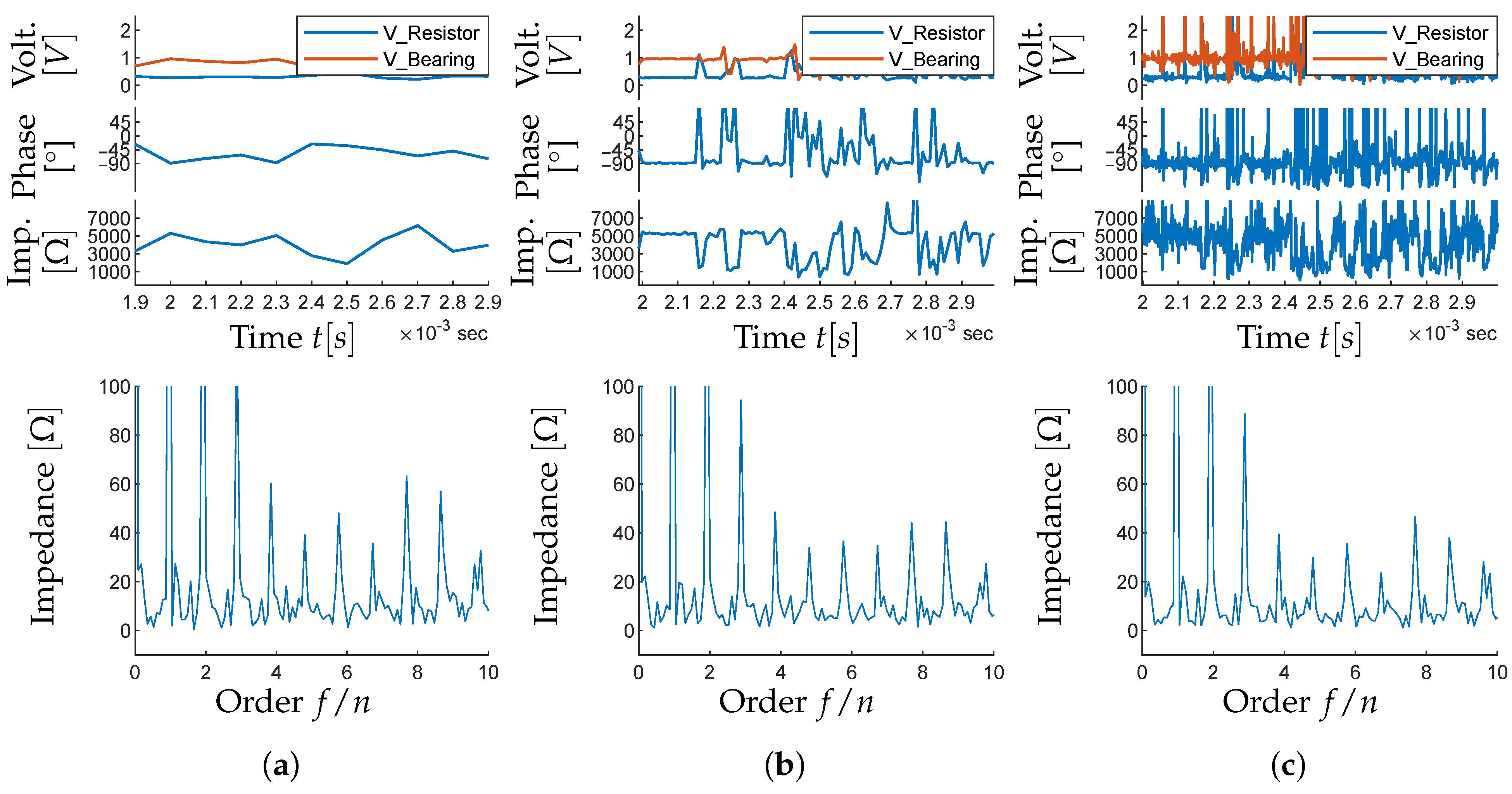
In order to investigate the influence of the window size on the measurement analysis, Figure 7 shows identical measurements taken at 1000 N and 1000 rpm with window sizes between ${10}^{-4}$ s and ${10}^{-6}$ s. The analysis is performed using a linear regression algorithm as the FFT analysis can only yield window sizes of up to ${10}^{-4}$ s, as described in Section 2.5.1. Figure 7a shows the first measurement at a window size of ${10}^{-4}$ s. That means for each ${10}^{-4}$ s, the measurement results are fed into a linear regression algorithm that fits the amplitude and the phase of a sine signal to the measurement results. The resulting sine functions describe the two voltages $V_{Resistor}$ and $V_{Bearing}$ from which the phase and the impedance are calculated. Therefore, each window yields exactly one value for phase and one value for impedance. For the plots in Figure 7, the time is plotted between 1.9 ms and 2.9 ms, which is kept constant for each of the subfigures. In subfigure (a), that means only ten measurement values are available for the phase and impedance plots. At 200 rpm, mixed lubrication is expected. However, within the selected time interval, the phase does not reach $0^{\circ }$ as would be expected during temporary metallic contact. This is because the contacts captured within this time frame are shorter than one window.

This becomes apparent in Figure 7b, in which the window size is reduced to ${10}^{-5}$ s. Now individual contacts are visible more clearly in the phase and impedance signal. One example is seen between $2.1$ ms and $2.2$ ms, which shows a period of metallic contact that can be identified by a reduction in impedance and an increase in phase towards $0^{\circ }$. It should be noted that the phase angle reaches positive values; however, that is the result of measurement inaccuracies at low impedances. A more realistic interpretation of the phase angle would be $0^{\circ }$. In subfigure (a), this contact is not noticeable, as one time window ranges from $2.1$ ms to $2.2$ ms and the contact is relatively short compared to the rest of the window at hydrodynamic lubrication. The contact only slightly increases the phase for the data point at $2.2$ ms in subfigure (a). Therefore, it can be said that larger window sizes act as a summarizing factor in which individual contacts are not noticeable within an analysis window.

Figure 7c shows the reduction of the window size to a more extreme case at ${10}^{-6}$ s. With the measurement frequency of 10 MHz, this means that each window only contains ten measurement points which are used for the regression algorithm. Consequently, the time resolution of the analysis is further improved and even shorter contacts are potentially still visible. However, that also means that inaccuracies play a more significant role as it is questionable how accurate a regression algorithm can be with only ten available measurement points with noise effects from the environment. This could be improved by increasing the measurement frequency but that also increases the size of the measurement data further. The noisy signal of subfigure (c) is not only the result of inaccuracies. Metallic contacts cause low impedance values, which create calculation inaccuracies and result in non-physical phase angles. Some of the noise in Figure 7c could be due to the fact that window sizes are small enough that individual contacts last for the full window length and consequently create non-physical phase angles and inaccurate impedance values. This can only be falsified with an increase in measurement frequency beyond 10 MHz.

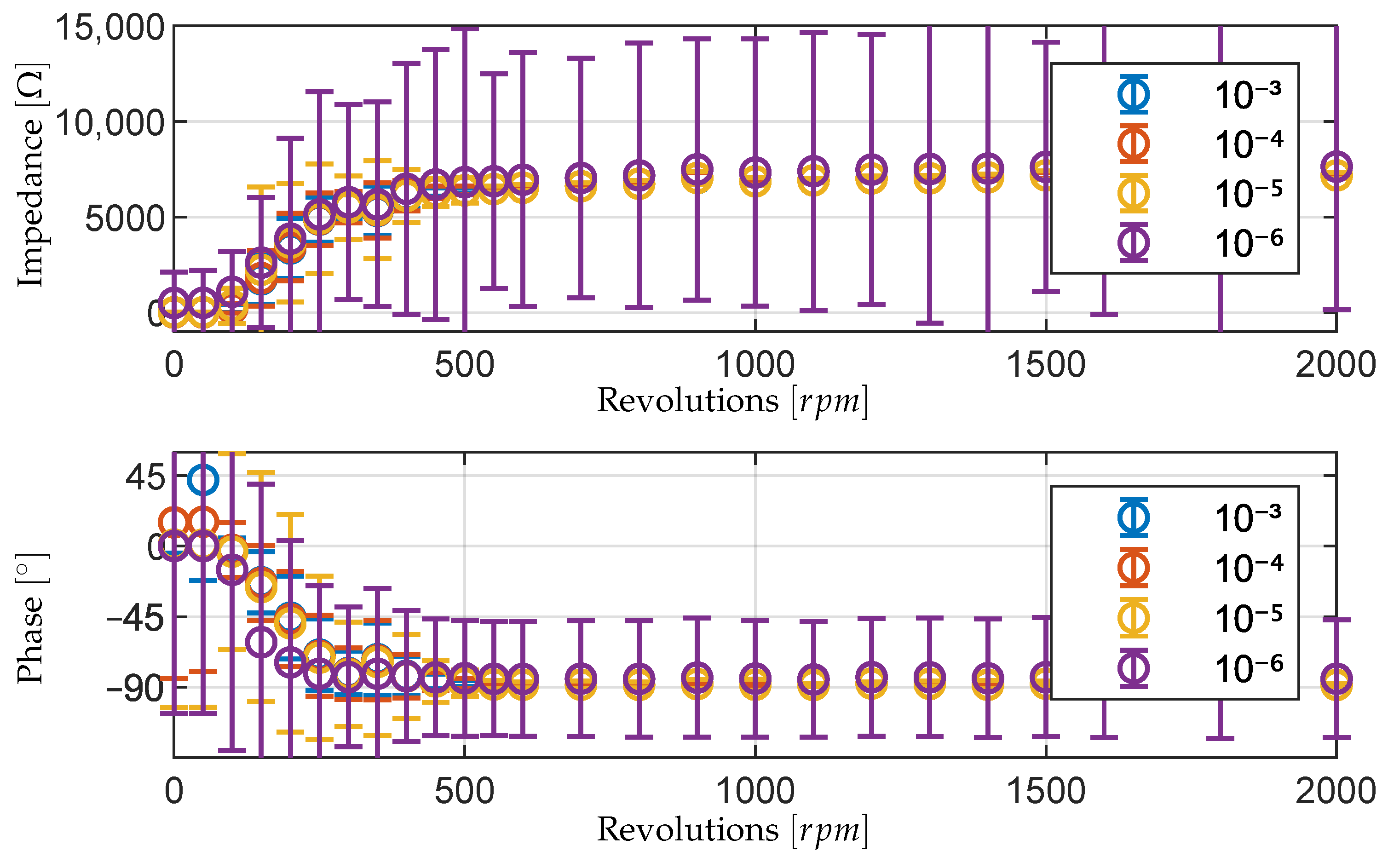
Figure 8 shows the summary of different time window sizes over the rpm range of the measurements by analyzing the measurements for each rpm step, calculating the mean and the standard deviation and plotting them as an errorbar plot. While all measurements generally show the same behavior, as would be expected, it is noticeable that the window size of ${10}^{-6}$ s causes a significant increase in standard deviation. Based on these results, the window size of ${10}^{-5}$ s seems to represent the best compromise between the detection of individual metallic contacts and reliability of the measurement. Since the FFT analysis can only reach window sizes of ${10}^{-4}$ s, the regression algorithm is to be preferred.

One tool for monitoring the amount of metallic contact when using impedance measurement is the PCT value (see Section 2.5.3). PCT analysis can be used in conjunction with the analysis described in this section to gain information about the ratio of metallic contact. However, as described by Hausmann et al. [5], PCT analysis is ambiguous and would require small window sizes to be accurate. For that reason, the next section discusses how the interpretation of the measurement results can be improved when mainly using PCT as a concept.

3.3. Physical Interpretation of Analyzed Data Using PCT Analysis

In this section, firstly, adaptations to the analysis methods are presented which allow an improvement to the precision of the PCT analysis when using AC signals in transient system behavior such as when changing from metallic contact to hydrodynamic lubrication temporarily. Secondly, the interpretation of an offset AC signal is performed to compare the suitability of AC signals and offset AC signals when measuring the electric behavior of journal bearings.

3.3.1. Behavior of PCT Analysis in Transient Systems

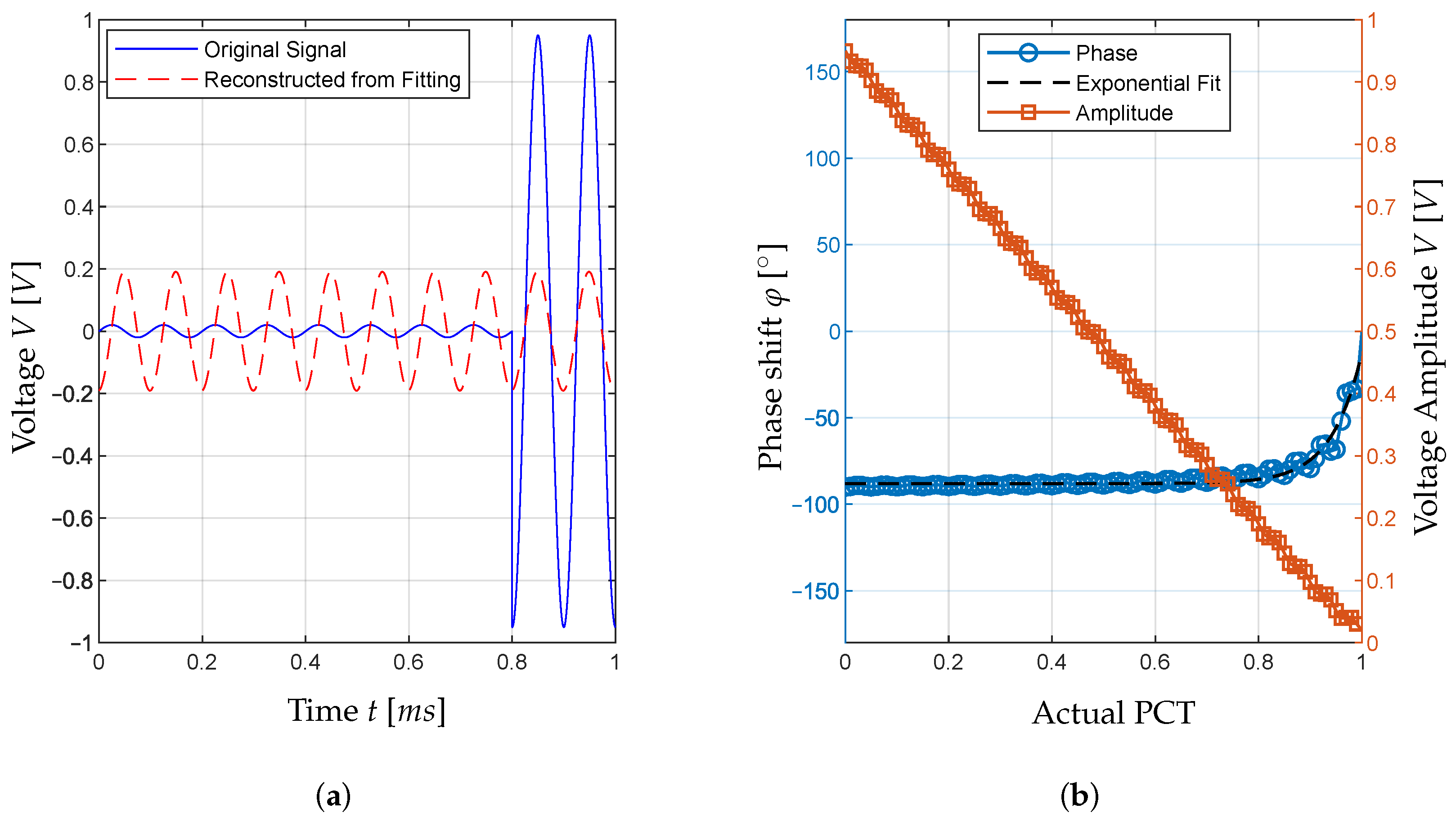
As described in Section 2.5.3, Hausmann et al. introduced a way to estimate the PCT value based on the phase angle and Equation (11) [5]. However, it is not known whether a linear estimation of the PCT value based on the phase angle represents an approximation of the actual PCT value. Therefore, a test is set up that simulates different PCT values of signals. For that purpose, a sine signal represented by Figure 9a is setup in MATLAB R2025b. The signal lasts for the length of one time window, as it would when FFT or regression analysis is used. The sine signal is described by Equation (7), with a peak value of $0.95$ V for hydrodynamic lubrication and $0.02$ V for boundary lubrication. The values are taken from measurements at the test bench to ensure that the simulated signal is representative. It is further assumed that the phase of the signal during hydrodynamic lubrication is shifted by $-{90}^{\circ }$ compared to the phase during boundary lubrication. The resulting signal can be written according to Equation (12). In this case, a PCT value of $0.8$ is assumed with metallic contact at first and hydrodynamic lubrication in the final $0.2$ ms.

$$y=\{\begin{array}{ccc}0.02\mathrm{V}·sin(2·\pi ·10\mathrm{kHz}·t+0^{\circ })& & \mathrm{if}t<0.8\mathrm{ms}\\ 0.95\mathrm{V}·sin(2·\pi ·10\mathrm{kHz}·t-{90}^{\circ })& & \mathrm{if}t\ge 0.8\mathrm{ms}\end{array}$$

(12)

This signal is analyzed using the regression analysis described before, although it should be noted that the choice between an FFT analysis and a regression analysis does not affect the results of the conclusions drawn in this section. The regression analysis leads to the reconstructed signal, which is also plotted in Figure 9a. As can be seen, the phase of the reconstructed signal does not visibly differ from the phase of the original signal during the final $0.2$ ms. However, the amplitude is significantly affected by the initial $0.8$ ms of the signal. The size of a time window does not affect the results presented here. Additionally, the order in which boundary and hydrodynamic lubrication occur or how often the behavior changes inside a time window does not alter the results.

To analyze the influence of the PCT value on the phase and the amplitude of the reconstructed signal, the calculations presented here are repeated for different PCT values. The result are then plotted in Figure 9b. As can be seen from the results, the phase of the reconstructed signal is at $-{90}^{\circ }$ for $PCT=0$. However, with an increase in the PCT value, the phase does not change significantly. This is due to the fact that the voltage amplitude at simulated hydrodynamic lubrication is larger by a factor of 50 compared to the amplitude during simulated boundary lubrication. Therefore, the phase at hydrodynamic lubrication dominates the analysis. This indicates that the phase is not a suitable variable to calculate the PCT value.

The amplitude behaves linearly between the different PCT values. Physically, the amplitude represents the magnitude of the impedance. If the estimation according to Hausmann et al. [5] (Equation (11)) is applied, it should be applied using the amplitude instead of the phase angle. For that, both amplitudes at boundary lubrication and hydrodynamic lubrication need to be known, which is not always possible, e.g., Hausmann et al. had no way to measure or estimate the amplitude of the measurement at hydrodynamic lubrication. In this case, the phase angle, which is known to be between $0^{\circ }$ and $-{90}^{\circ }$, is the only option. For that purpose, the function of the phase shift in Figure 9b is approximated using an exponential function in Equation (13) with the parameters $A,B,C$ and the $PCT$ value x. The parameters for the function of the phase shift in this contribution are calculated using the MATLAB function “fminsearch”. The resulting fit yields an RMSE value of ${2.79}^{\circ }$ and an R² value of $0.95$. The resulting exponential function is also shown in Figure 9b.

$$\begin{array}{cc}\hfill \phi & =A·e^{B·x}-C\mathrm{with}:\hfill \\ \hfill A& =2.78·{10}^{-6}\hfill \\ \hfill B& =17.12\hfill \\ \hfill C& =88.03\hfill \end{array}$$

(13)

In conclusion, it can be said that the calculation of the PCT value using the amplitude can be performed linearly. The calculation of the PCT value based on the phase angle can only be performed using an exponential function with parameters A, B and C being dependent on the ratio between the amplitudes at boundary lubrication and at hydrodynamic lubrication. That means that either those are known, in which case the PCT value can be calculated based on those, or that they are unknown, in which case they have to be estimated, leading to inaccuracies.

It should also be said that the conclusions drawn from the simulation here are based on the assumption of one crossover from simulated boundary to simulated hydrodynamic lubrication. In reality, the voltage signal will drop upon direct metallic contact and only slowly recharge, depending on the resistance and capacitance in the electric circuit. It is likely that individual contacts will occur briefly but multiple times per time window, which means that potentially a significant amount of time of the window will be spent while recharging the voltage. The results shown here don not account for that. However, they show the general behavior of the calculated phase and amplitude depending on the PCT, which allows a more accurate assessment of PCT values when using AC signals for impedance and capacitance measurements.

3.3.2. PCT Analysis of AC Signal Measurements

Based on the findings described in the previous section, a PCT analysis is performed on the measurements described in Figure 7. Figure 9 shows that the PCT analysis can be performed using the impedance or the phase. In this section, both analyses are conducted and compared to identify which one is preferable in practice.

Figure 10 shows the PCT analysis based on the magnitude of the impedance (Figure 10a). In this case, it is assumed that PCT equals 0 for the detachment point, which is selected manually based on the impedance signal at 550 rpm in which no individual contacts can be identified. It is also assumed to be 1 for the impedance of $0\Omega$. In between these two points, a linear function is assumed, as described in Equation (14). For investigation, the analysis is performed for different window sizes. As expected, it can be seen that the PCT analysis for the window sizes 1 ms, $0.1$ ms and ${10}^{-5}$ s are consistent and are overlapping. This indicates that the PCT analysis based on Equation (14) is now independent of the window size, which is an improvement to existing PCT analysis. The only influence the person performing the analysis still has lies in the selection of the reference value for hydrodynamic lubrication. However, with this analysis, the reference value of 550 rpm is a facts-based choice instead of an arbitrarily selected value.

$$PCT=\{\begin{array}{cc}1& \mathrm{if}\left|Z\right|\le 0\Omega \\ 1-{\displaystyle \frac{\left|Z\right|}{\left|Z\right(n=550\mathrm{rpm}\left)\right|}}& \mathrm{if}0\Omega \le \left|Z\right|\le \left|Z\right(n=550\mathrm{rpm}\left)\right|\\ 0& \mathrm{if}\left|Z\right|>\left|Z\right(n=550\mathrm{rpm}\left)\right|\end{array}$$

(14)

Figure 10b shows the PCT analysis performed based on the phase shift between the two measured voltage signals, as conducted by Hausmann et al. [5]. However, since it is now known that the phase is not a linear equation, the analysis is performed by inverting Equation (13) with the parameters A, B and C. As can be seen from Figure 10b, the results are dependent on the window size and are scattered. This is due to the exponential equation creating significant changes in PCT, with small deviations in the observed impedances. This becomes more apparent when looking at Figure 11.

$$PCT=\{\begin{array}{cc}0& \mathrm{if}\phi \le -{88.03}^{\circ }\\ {\displaystyle \frac{1}{B}}·ln\left({\displaystyle \frac{\phi +C}{A}}\right)& \mathrm{if}-{88.03}^{\circ }\le \phi \le 0^{\circ }\\ 1& \mathrm{if}\phi >0^{\circ }|\end{array}$$

(15)

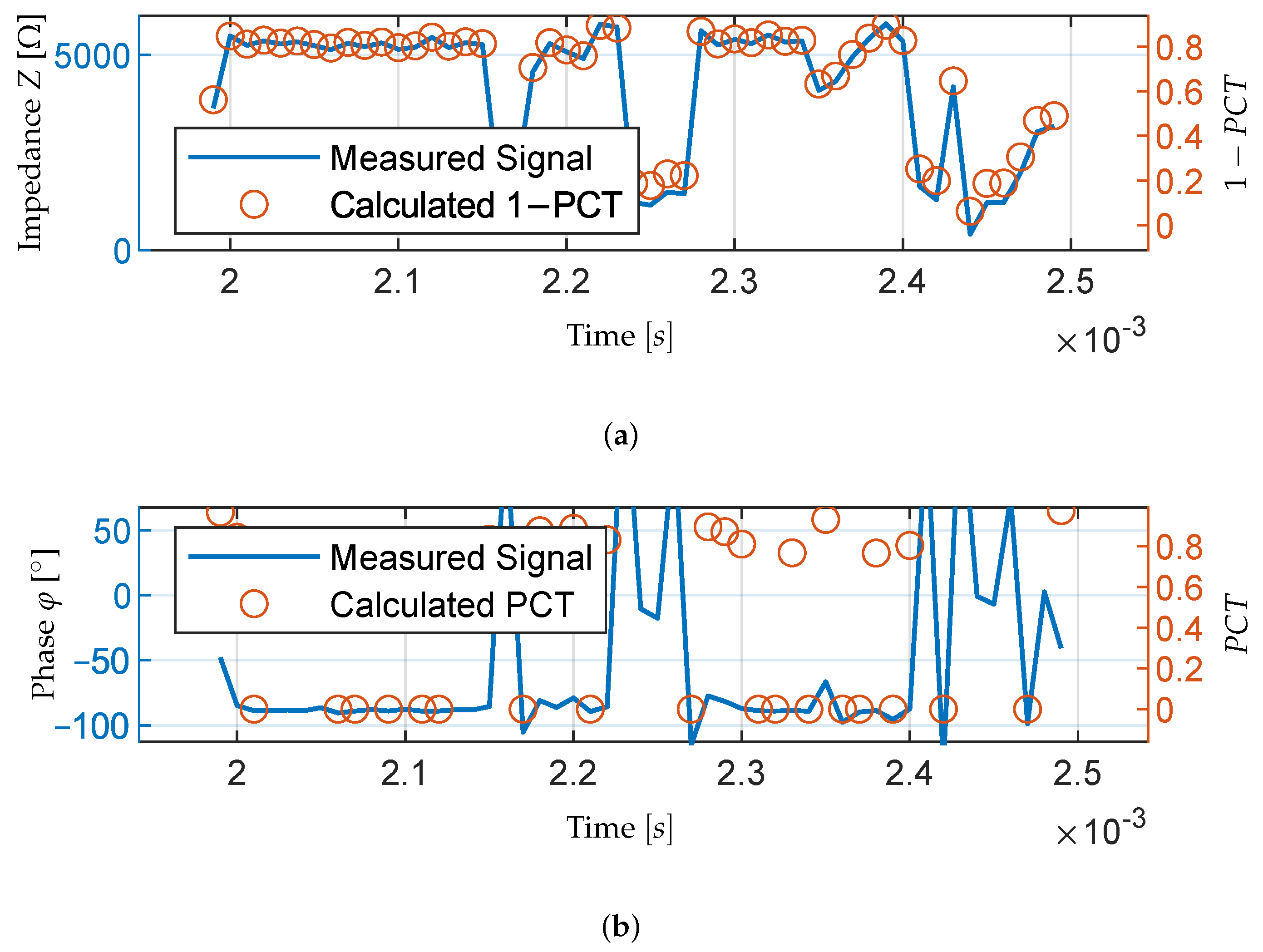
Figure 11 shows the same PCT analysis performed for a short impedance signal. The impedance and phase curves are the same as those used in Figure 7 but additionally, the PCT values for each window are added with a second y-axis. Figure 11a uses the inverse PCT value simply due to the fact that PCT and impedance are inversely proportional, as higher impedance values imply lower PCT values. This way, both values can be compared within one picture.

Figure 11 shows a good correlation of PCT and impedance values. It can be seen that even at 200 rpm, the signal temporarily indicates hydrodynamic lubrication but is disrupted by momentary metallic contact. With this analysis, it is possible to achieve a reliable PCT analysis with relatively large window sizes. One disadvantage is that the PCT value of 1 is difficult to reach as the reference value for this is taken from the detachment point at higher rotation rates. However, this is still a significant improvement compared to existing PCT analyses.

As Figure 11b shows, this is not possible for the phase analysis despite the good fit of parameter R² of $0.95$ and the low RMSE value of ${2.79}^{\circ }$. This is due to a multitude of factors. Firstly, the phase angle is more prone to show non-physical values due to inaccuracies at low impedances, as can be seen by the phase curve indicating positive values at multiple contact points. Due to the discontinuity of Equation (15), this leads to jumps in the PCT value. Additionally, Equation (15) is only defined for $\phi >-{88.03}^{\circ }$ as this is the value of parameter C. Any phase angle below $-{88.03}^{\circ }$ yields $PCT=0$, while $-{88.02}^{\circ }$ yields $PCT=0.48$, a significant change in PCT value despite almost no change in the phase. However, we also know from Section 3.3.1 that assuming a linear equation is not a valid alternative.

In summary, the analysis shows that impedance-based PCT calculations yield reliable results which are only dependent on the selection of the reference value. This still yields inaccuracies but is significantly more reliable than PCT analyses based on the phase.

3.4. PCT Analysis of Offset AC Signals

As discussed in previous sections, the PCT analysis of an offset signal in principle promises to alleviate the problems of the PCT analysis of an AC signal. To verify that hypothesis, an offset measurement is analyzed in this chapter.

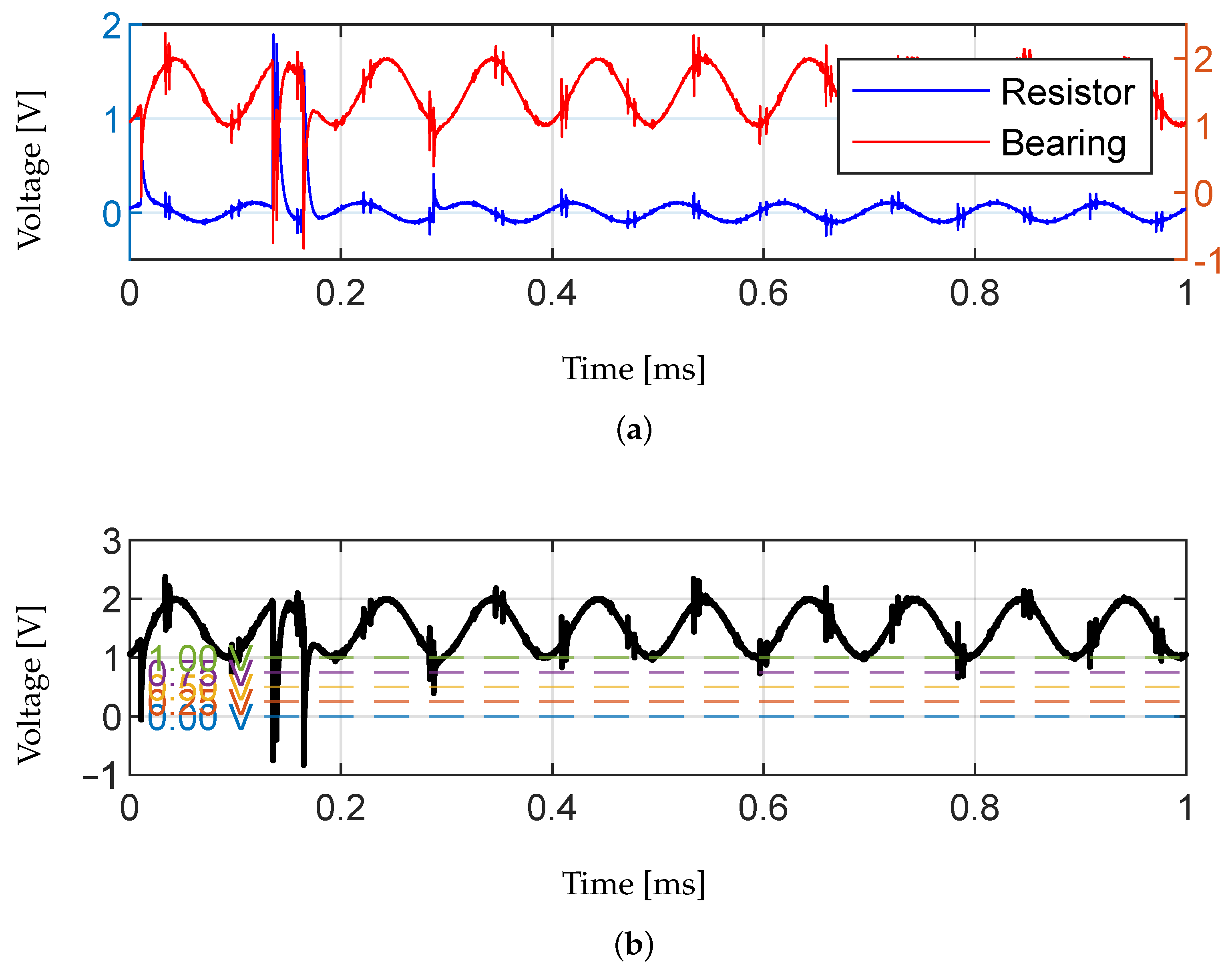
Figure 12a shows such an offset measurement at 1300 rpm. As before, the resistor and bearing of the voltage divider are shown over a time frame. An offset signal is a superposition of a constant DC signal and an AC signal. For the DC signal, the capacitance of the bearing represents an infinite resistance. Consequently, the DC part of the offset signal only drops off over the capacitance and is not present in the resistance signal. In Figure 12, one metallic contact can be seen representing an individual contact just before $0.2$ ms, with the voltage over the capacitance dropping off and the voltage over the resistance rising. During the contact, the voltage over the resistance rises to almost 2 V as for a brief time, the voltage drops entirely over the resistor and not the bearing.

In Figure 12b, the concept of a PCT analysis is visualized using threshold values between 0 V and 1 V. When the voltage signal is below the threshold value, a metallic contact is assumed. The duration of each contact is measured and used to calculate the PCT. It is, however, not obvious which threshold value is to be used as in theory, any voltage below 1 V represents a metallic contact. The metallic contact before $0.2$ s can be identified by each of the threshold values. However, in the event of a metallic contact, the capacitance of the bearing discharges and has to be recharged. During the charge, the voltage drop over the bearing rises continuously above 1 V over the course of approximately $15\mathsf{\mu }$s. The PCT analysis currently cannot account for the charging time. This will result in varying PCT results depending on which threshold value is used. Furthermore, just before $0.3$ ms, it can be seen that signal noise creates a drop in voltage likely caused by the inverter of the electric motor. Depending on which threshold value is used, this deviation can influence the PCT value. Therefore, the selection of the threshold value has an influence on the calculated PCT. Another question that remains is whether the measurement frequency has an influence on the PCT analysis, as discussed in previous sections.

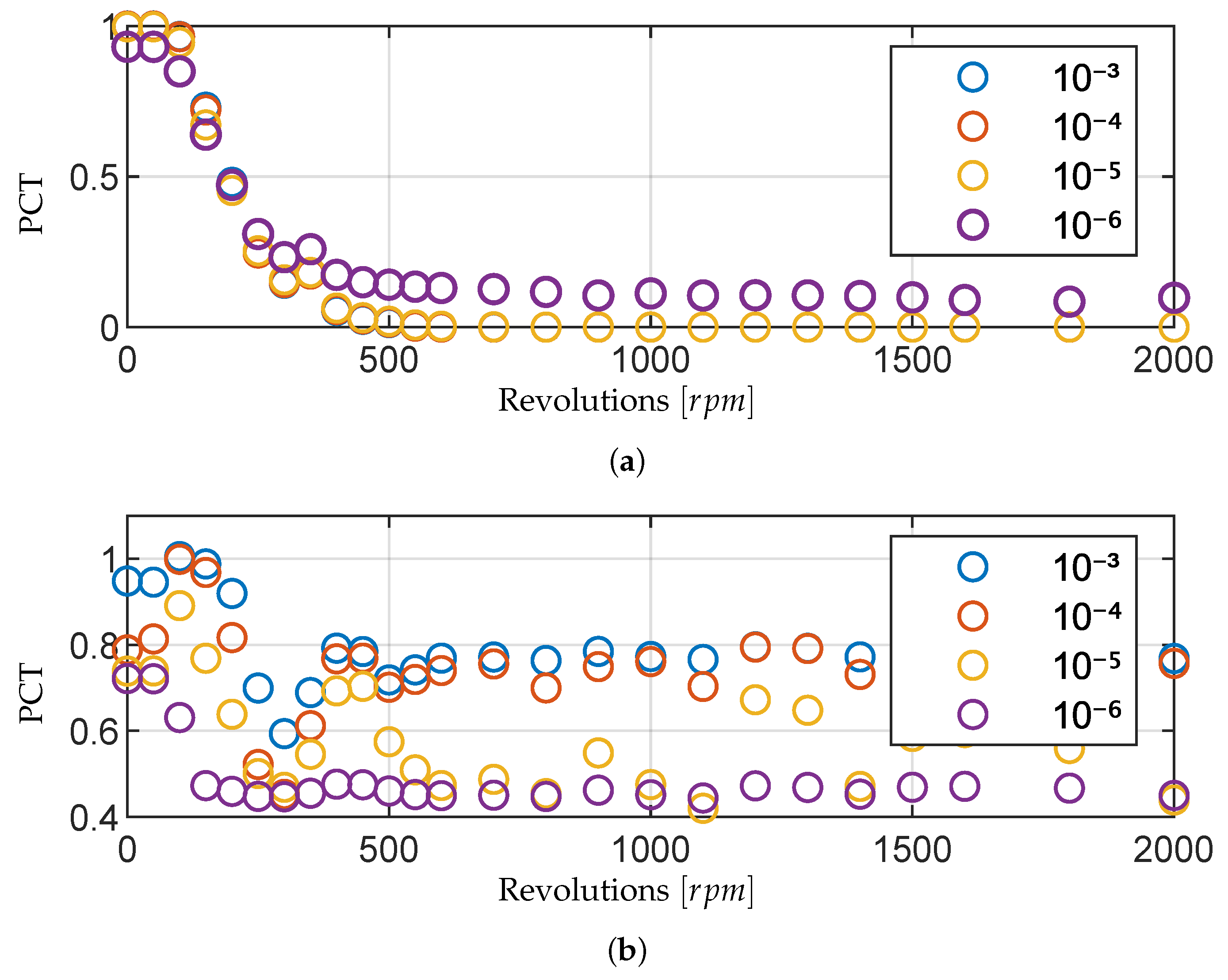
To answer this question, Figure 13a shows the PCT analysis using the threshold value of $0.5$ V and varying measurement frequencies. The PCT value is calculated by taking identical measurements and artificially reducing the measurement frequency by calculating the mean of multiple measurement points to represent the measurement frequencies of 1 kHz to 10 MHz. It should be noted that the measurement shows an unexpected jump in PCT between 300 rpm and 400 rpm; however, this is due to the complex behavior of bearings in mixed lubrication. Minor changes in the test bench parameters like temperature or lubricant pressure can cause significant changes in the lubrication film thickness in mixed lubrication. The focus of this section is not to analyze this discrepancy but the consistency of the PCT analysis of offset signals.

Figure 13a shows a good fit of different measurement frequencies, implying that the frequency itself does not have a significant impact on the calculated PCT. This can be compared to Figure 7, where the measurement frequency significantly alters the observed contact events and thus would impact the calculated PCT. This can only be compensated to some degree by the analysis presented in Section 3.3.2. This does not have to be performed when using offset measurements.

Figure 13b shows the impact of the threshold values as presented in Figure 12b at the maximum measurement frequency of 10 MHz. The selection of the threshold parameter determines the calculated PCT value and influences any conclusions that could be drawn from the value significantly. Taking the threshold value of 0 V would indicate that metallic contact only occurs for 50% of the running time, even at 50 rpm. This is clearly non-physical as the bearing stays in contact 100% of the time at slow rotation rates. However, we also know that 1 V is susceptible to noise which can influence the calculated value, as can be seen in Figure 12b. Potentially, the most promising threshold value is $0.5$ V due to it being the median between both sources for errors. However, at this point, no definitive answer to this question can be given. Due to this problem, the PCT analysis of an offset signal offers no significant advantage over the analysis discussed in Section 3.3.2.

4. Discussion

In this contribution, the measurement setup for the measurement of the electric behavior of journal bearings consisting of possible electric circuit setups, electric signal types and data analysis methods was discussed. For that purpose, initially, a selection of electric circuit types and electric signal types were identified based on theoretical assessments of their suitability. Measurements were then taken using a voltage divider setup with AC signals and offset AC signals and analysis methods analyzed their suitability. The results showed that FFT and linear regression algorithms can both deliver identical results when used to derive the amplitude and phase of a sine signal. However, linear regression in allow time windows to be analyzed that are smaller than the period of the electric AC signal, something which FFT analysis does not allow. A regression algorithm is therefore the better tool to identify the phase and amplitude of sine signals in impedance measurements.

Additionally, the resulting impedance obtained using a linear regression algorithm are interpreted using PCT analysis. For that purpose, a simulation was set up to analyze the behavior of the PCT value when the electric behavior of the bearing changes within a time window. Based on this, equations were derived to calculate the PCT value despite the transient behavior inside a time window during mixed lubrication. The PCT analysis was then carried out for real measurements and it was shown that PCT calculations based on the amplitude of the sine signals yield consistent and reliable results compared to a PCT calculation based on the phase. Inaccuracies remain because the results are dependent on the determination of the detachment point, but they are significantly smaller than previous PCT analyses based on the phase, as conducted by Hausmann et al. [5].

Lastly, the suitability of offset AC signals for PCT assessments was investigated. The results showed that PCT assessment is largely independent of the measurement frequency but highly dependent on the selection of the reference value. An offset signal therefore does not offer advantages over a PCT assessment performed using AC signals without offset but it complicates the linear regression algorithm. Therefore, AC signals are to be preferred over offset AC signals.

5. Conclusions

With the knowledge presented here, a measurement setup and data analysis method can be selected for the electrical monitoring of journal bearing lubrication films. Additionally, a PCT assessment is available which allows the physical interpretation of the results obtained. These results may allow the implementation of predicting wear and identifying critical operation conditions in future. However, some inaccuracies remain in the PCT analysis and a verification of the results is not possible as the true contact time during operation is not measurable.

The conclusions can also be transferred to other applications of monitoring the lubricated contact, such as for rolling-element bearings and gear contacts. While the monitored capacitance will differ and will require individual modeling, the setup and approach presented here are transferable. The physical interpretation of electrically monitored tribological contacts in general can also benefit from the findings presented here. However, it should be noted that the simplifications made in Section 2.4 need to be checked critically as they are likely to lead to inaccurate results when the observed capacitance differs significantly from the capacitance range observed here.