Communication

A Fully Implicit Coupled Scheme for Mixed Elastohydrodynamic Problems on Co-Allocated Grids

by
Sören Wettmarshausen
* and
Hubert Schwarze
Institute of Tribology and Energy Conversion Machinery, Clausthal University of Technology, 38678 Clausthal-Zellerfeld, Germany
*
Author to whom correspondence should be addressed.
Lubricants 2024, 12(9), 322; https://doi.org/10.3390/lubricants12090322
Submission received: 26 June 2024 / Revised: 9 September 2024 / Accepted: 16 September 2024 / Published: 19 September 2024
(This article belongs to the Special Issue Advances in Mixed Lubrication)

Abstract

:
In the modeling of elastohydrodynamic lubrication problems considering mixed friction, strongly coupled dependencies occur due to piezo-viscous effects and asperities, which can make a numerical solution exceptionally difficult. A fully implicit coupled scheme for solving mixed elastohydrodynamic lubrication problems is presented. Our scheme uses finite-volume discretization and co-allocated grids for hydrodynamic pressure and elastic deformation. To provide strong coupling between pressure and deformation even in the highly loaded zone, a correction term that adds numerical diffusion is used. The resulting linear equation system of this scheme can be efficiently solved by Krylov subspace methods. This results in an improved accuracy and computational efficiency compared to the existing methods. This approach was validated and has been shown to be accurate.

Graphical Abstract

1. Introduction

Mixed elastohydrodynamic lubrication (EHL) is a mechanism found in many tribological problems. Analysis of EHL problems is essential for the operational reliability and performance of a wide range of applications in mechanical and medical engineering. In modeling EHL problems, the interaction between elastic deformations of solids and the flow of a viscous lubricant leads to complex and strongly coupled dependencies. Due to piezo-viscous effects, the viscosity varies by many orders of magnitude for highly loaded contacts. The resulting poor conditioning of the problem makes a numerical solution exceptionally difficult and requires efficient and stable computational methods. A solution for EHL contact was first proposed by Hamrock and Dowson [1] using the Gauss–Seidel method. Later, a solution technique using geometric multigrid methods was developed by Venner [2]. Hughes presented a coupled solution for pressure and deformation using a differential deflection method [3]. In [4] A Computer Program Package for mixed elasto-hydrodynamic lubrication is presented. A coupled solution procedure is introduced by [5] using a finite element approach and a direct solver for the linearized system of equations. To handle stability issues, a streamline upwind/Petrov–Galerkin formulation introduced in [6] that adds numerical diffusion is used. A solution procedure for elasto-hydrodynamic lubrication problems based on the Navier-Stokes equations is presented in [7] and a solution procedure with a coupled solution of a structural model and the Reynolds equation for elastohydrodynamic contacts is described in [8]. Khonsari describes a numerical model for mixed EHL contact with inner and outer loops [9]. In [10], the solution for mixed EHL problems was described using an iterative scheme, and later, in [11], cavitation was also considered using an iterative scheme. In this work, a new approach to overcoming these challenges for mixed EHL problems is presented through a fully implicit coupled scheme. This scheme provides strong coupling between hydrodynamic pressure and deformation and works on co-allocated grids.

2. The Mathematical Model

2.1. Governing Equations

2.1.1. Average Reynolds Equation

The EHL contact is described by a pressure field, a deformation field, and rigid body displacement. These variables are specified by solving governing equations. To determine the hydrodynamic pressure, the average Reynolds equation introduced in [12] by Patir and Cheng is used. Unlike Patir and Cheng, we use a generalized formulation for compressible fluids.
f p : = · ρ θ h 3 12 η Φ p p · ρ θ h U 1 + U 2 2 · ρ θ h Φ s U 2 U 1 2 ( ρ θ h ) t = 0
In a Cartesian coordinate system, the flow factor tensors for pressure Φ p and shear flow Φ s have the components
Φ p = Φ p x 0 0 Φ p y , Φ s = Φ s x 0 0 Φ s y .
The flow factors are determined separately. This can be done by interpolating from table values, which is done in this work, or by evaluating an empirical correlation, for example [12,13]. In the case of smooth surfaces, the average Reynolds equation simplifies by Φ p = 1 and Φ s = 0 .

2.1.2. Film Thickness Equation

Assuming that two arbitrarily shaped bodies are in contact in a sufficiently small area, the shape of these bodies can be approximated by an ellipsoid with two radii. The distance between these bodies can be expressed as a sum of the gap height from the curvature, the change by deformation w, and the rigid body displacement h 0 . From this, a function for the determination of h is derived:
f w : = h x 2 2 R x + y 2 2 R y + w + h 0 = 0
with the auxiliary radii R x = R 1 x R 2 x R 1 x + R 2 x and R y = R 1 y R 2 y R 1 y + R 2 y .

2.1.3. The Force Balance Equation

Furthermore, another equation is needed to determine the displacement. For this purpose, a predefined load condition is balanced.
f h 0 : = Ω p + p c d x d y F = 0
The contact pressure p c ( h ) is a function of the averaged gap height and can also be interpolated from table values. For smooth surfaces, p c = 0 everywhere.

2.2. Equation of State

For the treatment of the lubricant’s compressibility, the density pressure relation given by Dowson and Higginson [14] is used.
ρ = ρ 0 5.9 × 10 8 P a + 1.34 p 5.9 × 10 8 P a + p
Without considering cavitation, negative pressures occur in the solution. In early publications, these negative pressures were set to zero after the solution process [2]. This resulted in a discontinuous pressure gradient, which led to violation of the conservation of mass and could lead to numerical instability. In particular, it cannot be treated implicitly. Later publications have used a penalty function introduced by [15]. Other authors use Elrod’s cavitation algorithm, which is mass-conserving but, beyond that, is not physically motivated and cannot be treated implicitly either because the relationship between pressure and density is non differentiable. Our cavitation approach is mass-conserving and physically motivated and can be treated implicitly. The relation for fractional film content that incorporates the influence of cavitation effects and is motivated by pseudo cavitation is
θ = 1 + α B 1 + α B p a p .
Here, α B = 0.08 0.1 is the Bunsen solubility coefficient, p a is the atmospheric pressure. In EHL, the influence of α B on the results is negligible. The use of Elrod’s cavitation algorithm [16] is also possible in principle, but it cannot be linearized. In this context, α B can be interpreted as a numerical parameter. For α B 0 , the relationship is equivalent to Elrod’s cavitation algorithm with zero cavitation pressure.

2.3. Viscosity–Pressure Relation

There are several models for describing the viscosity–pressure relation. The simplest is the one by Barus.
η = η 0 e x p ( α p )
where η 0 is the reference viscosity, and α = 1 2.2 × 10 8 P a 1 is the pressure–viscosity coefficient for common lubricants. For a high pressure, this equation predicts an enormous and progressive increase in viscosity. However, experiments show a degressive correlation [17]. So, a better approximation can be obtained using the expression from Roelands [18].
η = η 0 e x p l n ( η 0 ) + 9.67 1 + p p 0 z 1
where p 0 = 1.98 × 10 8 Pa is the reference pressure. The exponent z can be computed from the well-known pressure–viscosity coefficient by
z = α p l n ( η 0 ) + 9.67 .

2.4. Elastic Deformation

To determine the elastic deformation of the two surfaces, the Boussinesq equation for the elastic half-space
w = 2 π E Ω p + p c ( x ξ ) 2 + ( y η ) 2 d ξ d η
is used, where E is the reduced Young’s modulus, which is defined by 2 E = 1 ν 1 2 E 1 + 1 ν 2 2 E 2 .

3. Spatial and Temporal Discretization

The equations presented above are now solved approximately using numerical methods. In the following, the spatial discretization of the model equations is performed on a Cartesian grid with m × n cells with extensions of Δ x and Δ y for interior cells and Δ x / 2 and Δ y / 2 at the boundary.

3.1. The Average Reynolds Equation

Written as an integral over a domain Ω , the Reynolds Equation (1) is
Ω ρ θ h 3 12 η Φ p p · n ^ d C Ω ρ θ h U 1 + U 2 2 · n ^ d C Ω ρ θ h Φ s U 2 U 2 2 · n ^ d C Ω ( ρ θ h ) t d A = 0
and after discretization, the three flux terms read in general as
Ω ρ θ h 3 12 η Φ p p · n ^ d C = f ρ ¯ θ ¯ f h ¯ f 3 12 η ¯ f Φ ¯ p f p f + d p f p ¯ f · n f
Ω ρ θ h U 1 + U 2 2 · n ^ d C = f ρ ˜ f θ ˜ f h ¯ f U 1 + U 2 2 · n f
Ω ρ θ h Φ s U 2 U 2 2 · n ^ d C = f ρ ˜ f θ ˜ f h ¯ f Φ ¯ s f U 2 U 1 2 · n f
where the subscript ( ) f means that the variable is evaluated at the face f. h ¯ f , η ¯ f , ρ ¯ f , θ ¯ f , Φ ¯ p f , and Φ ¯ s f are linear interpolations from the nodal values to f, and ρ ˜ f and θ ˜ f are the values from the upwind node. The gradient p f is an approximation at f like the central difference, and p ¯ f is an interpolation from approximations of the gradient at the nodes to f. The additional second term in (12) is a correction that adds numerical diffusion and guarantees strong coupling between hydrodynamic pressure and deformation. It can be shown that this term vanishes when the pressure varies as a second-order polynomial Appendix A. Higher-order pressure oscillations will be damped rapidly. This technique is known as ”Rhie-Chow interpolation” from the pressure-velocity coupling in the solution of the Navier-Stokes equations. Thereby, the term is motivated by the condition of continuity, and the coefficient d is approximated from the momentum equation [19]. In this case, d has to be approximated so that the correction is effective even in the high-pressure zone with large values for η . So,
d : = λ ρ 0 h 0 3 12 η 0
is proposed, where λ is an optional empirical factor. In the following, the discretization is evaluated for the grid shown in Figure 1. For this, we have the faces f = { w , e , s , n } , and the face normal vectors are n f = Δ y 0 , Δ y 0 , 0 Δ x , 0 Δ x . The linear interpolation example for the film thickness is h ¯ f = h P + h n b 2 with the central node P and its neighbor nodes n b = { W , E , S , N } . The pressure gradient approximation as an example at the face w is p f · n w = Δ y Δ x ( p P p W ) , and the interpolation from the approximations at the nodes is p w ¯ · n w = 1 2 ( p P + p W ) · n w with the approximations at the nodes p P · n w = Δ y 2 Δ x ( p E p W ) and p W · n w = Δ y 2 Δ x ( p P p W W ) . A similar procedure is used for the remaining faces. In sum, the correction term is
f d p f p ¯ f · n f = d Δ y Δ x 3 2 p P p W p E + 1 4 p W W + 1 4 p E E + d Δ x Δ y 3 2 p P p S p N + 1 4 p S S + 1 4 p N N .
The discretization of the temporal term is
Ω ( ρ θ h ) t n d A = Δ x Δ y Δ t ρ P θ P h P ρ P 0 θ P 0 h P 0
for the first-order backward Euler scheme and
Ω ( ρ θ h ) t n d A = Δ x Δ y 2 Δ t 3 ρ P θ P h P 4 ρ P 0 θ P 0 h P 0 + ρ P 00 θ P 00 h P 00
for the second-order backward Euler scheme, where ( ) 0 denotes a value from the last time step and ( ) 00 a value from the second last time step.

3.2. The Film Thickness Equation

Assuming that the pressure at the boundaries vanishes, (10) in the discretized form is
w i , j = k = 2 m 1 l = 2 n 1 K i , j , k , l ( p k , l + p c , k , l )
whereby
K i , j , k , l = 2 π E x i ξ k Δ x 2 x i ξ k + Δ x 2 y i η k Δ y 2 y i η k + Δ y 2 1 ( x i ξ ) 2 + ( y i η ) 2 d ξ d η
is the kernel of the elastic deformations. On an equidistant Cartesian grid, there are redundancies that can be used to reduce the size of K. With x p = | x i x k | and y q = | y j y l | , the kernel is
K p , q = 2 π E x p Δ x 2 x p + Δ x 2 y q Δ y 2 y q + Δ y 2 1 ( x p ξ ) 2 + ( y q η ) 2 d ξ d η
and the elastic deformation reads as
w i , j = k = 1 m l = 1 n K i k , j l ( p k , l + p c , k , l )
The evaluation of these integrals is
K p , q = 2 π E | y + | a s i n h x + y + + | x + | a s i n h y + x + | y + | a s i n h x y + | x | a s i n h y + x | y | a s i n h x + y | x + | a s i n h y x + | y | a s i n h x y + | x | a s i n h y x
with x + = x p + Δ x / 2 , x = x p Δ x / 2 , y + = y q + Δ y / 2 and y = y q Δ y / 2 [2].

3.3. The Force Balance Equation

The discretized force balance equation reads as
f h 0 = i = 2 m 1 j = 2 n 1 ( p i j + p i j , c ) Δ x Δ y F = 0

4. Solution Strategy

4.1. The Coupled System of Equations

The numerical discretization provides a non-linear system of equations. For the coupled solution for all the equations, the general equation system f ( X ) = [ f p , f w , f h 0 ] T = 0 is defined with the general solution variable X = [ p , w , h 0 ] T , which has the dimensions ( 2 m n + 1 ) × 1 . For the solution of this non-linear system of equations, the Newton–Raphson method is used. Starting from a previous solution, a better solution can be found by
X i , k + 1 = X i , k + Δ X i , k + 1 = X i , k J i j , k 1 f i , k
with the Jacobian
J = f p p f p w f p h 0 f w p f w w f w h 0 f h 0 p f h 0 w f h 0 h 0
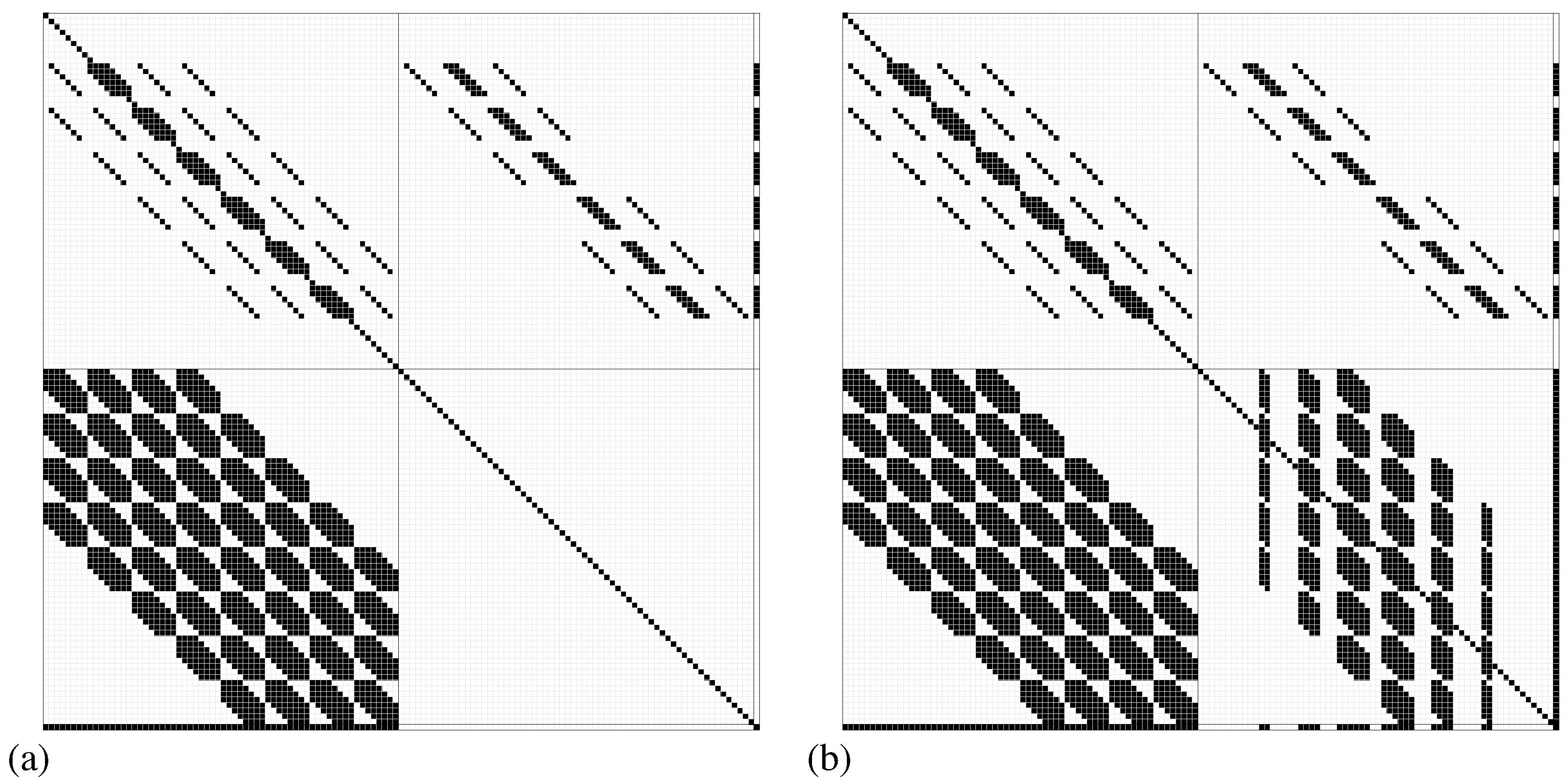
For simplicity and generality, the derivatives are evaluated numerically by forward differences. As the step size, ε X t y p i c a l is used, where ε is the machine accuracy and X t y p i c a l , i 0 is a typical expected value for X i . For the pressure and the deformation, the maximum values p H and d H from the Hertzian contact ellipse [20] can be used as X t y p i c a l . For the displacement, h c d H can be used. For better numerical efficiency, a sparsity pattern can be used when evaluating the Jacobian. This is shown in Figure 2. It can be seen that f p p is always banded, and f w p is always strongly populated. f w w is diagonal for smooth surfaces and strongly populated for rough surfaces. Furthermore, it is not necessary to re-compute the Jacobian for every iteration. Only at the beginning of the solution process when the change in the solution vector is high are the non-linearity and thus the change in the Jacobian significant. A simple and efficient way is to retain the Jacobian when all the residuals decrease at an acceptable rate.

4.2. The Relaxation Scheme

Relaxation of the solution is implemented in two different ways, one implicit and one explicit. For the deformation and displacement, an implicit scheme is utilized by adding a part to the diagonal of the Jacobian.
J i , i = J i , i 1 ω i 1 f i X t y p i c a l , i
Here, ω w = 1 and ω h 0 = 0.3 are used. This procedure guarantees sufficient large diagonal elements for the deformation and displacement so that the linear equation sytem can be solved by the iterative solver. For the pressure equation this is guaranteed by the correction term, and ω p = 1 is used for the pressure, but explicit relaxation is used with
Δ X i , k + 1 = β i Δ X i , k + 1 *
with β p = 0.5 . For the deformation and displacement, β w = β h 0 = 1 is used.

4.3. The Linear Equation Solution

Before solving the system of equations, each equation is scaled by its pivot element for better conditioning:
f i * = f i J i , i , J i , j * = J i , j J i , i
The final system of linear equations J i j , k * Δ X i , k + 1 * = f i , k * can be solved efficiently with iterative solvers like Krylov subspace methods. Combining this with the Newton–Raphson method is also known as the Newton–Krylov method. Here, BiCGSTAB is used with ILU as the preconditioner [21].

4.4. Initialisation

The values for the pressure and the deformation can be initialized with zeros. The rigid body displacement can be initialized with the central film thickness by the Hamrock–Dowson method [1].
h c D = 1.69 G 0.53 U 0.67 W 2 0.067 ( 1 0.61 e 0.73 k ) R x
with W 2 = w E R x 2 , U = η 0 ( U 1 + U 2 ) E R x , G = α E and k = 1.03 R y R x 0.64

5. Numerical Results

5.1. Test Case

The method developed was then analyzed using test examples. For validation, a test case (smooth case) according to Venner [2] was used. The parameters and the numerics used are listed in Table 1. These values are used for both smooth and rough cases.
Here, a and b are the values for the Hertzian contact ellipse [20].

5.2. Surface Roughnes

To create the rough case, flow factors and contact pressure were determined for a pair of randomly generated synthetic surfaces with a given height probability distribution (tangent function) and autocorrelation function. The surfaces were generated by correlating Gaussian random numbers with an exponential autocorrelation function and then correcting the height distribution to fulfil the specified characteristics. For details on the surface generation, see [23,24]. The surfaces have the characteristics of the Abbott–Firestone curve R k = 0.3 μm, R p k = R v k = 0.15 μm, which results in a average roughness of R a = 0.1 μm, a quadratic mean roughness of R q = 0.13 μm, a kurtosis of K = 3 , and a skewness of S k = 0 . The correlation function is isotropic with a correlation length of λ 0.5 = 5 μm.
The surface roughness as well as the flow factors and the contact pressure are shown in Figure 3 and listed in Table 2. In the following, the results are shown for this case.

5.3. Mesh Study

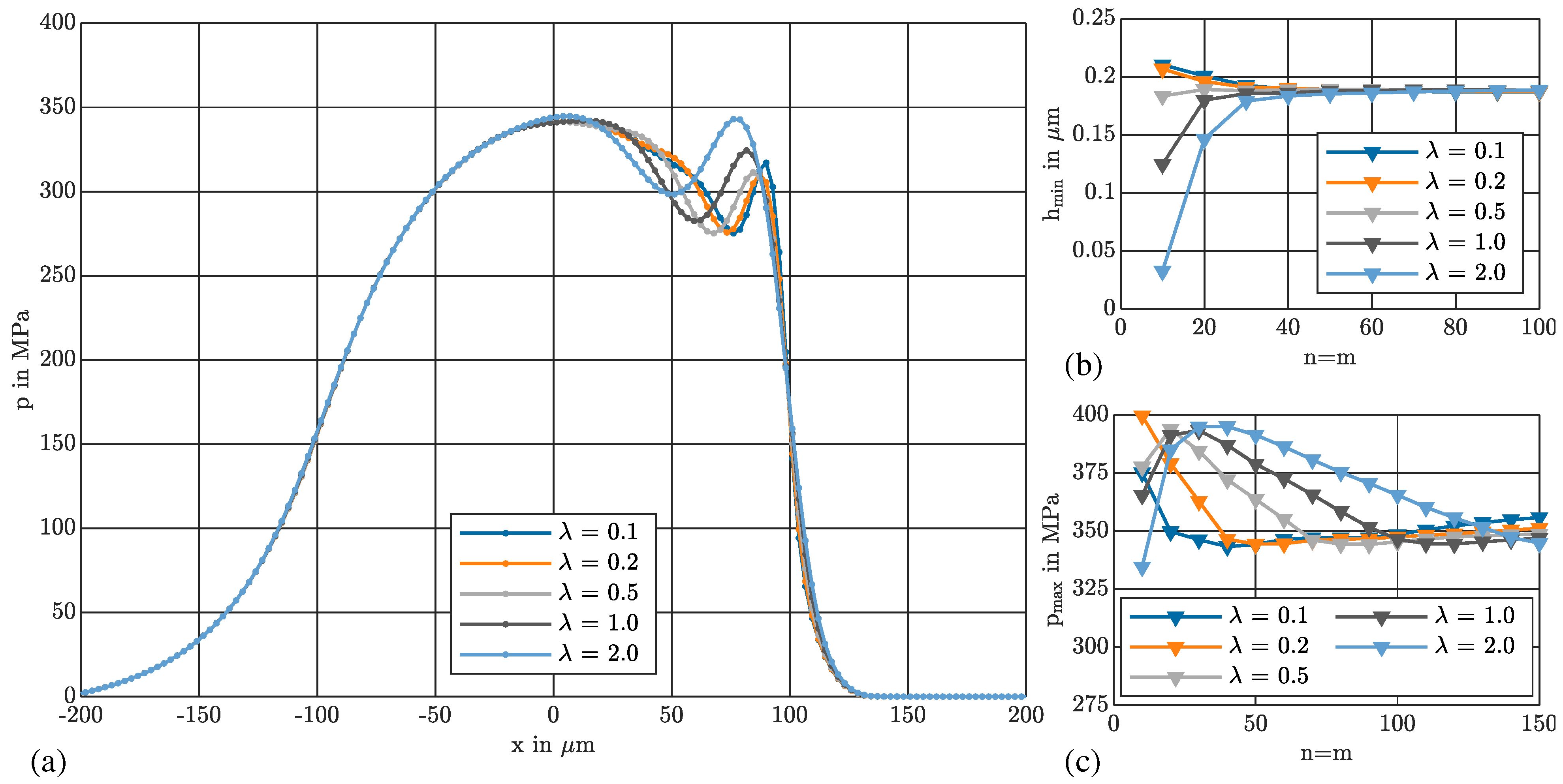
The magnitude of the correction term in (12) depends on the grid spacing via the accuracy of the approximations of the pressure gradient. If the approximations are exact, the correction term has no influence on the solution. So, the choice of λ and the number of grid points are not independent. In Figure 4a, the pressure distribution is shown for n = m = 150 and different values of λ .
A smaller lambda value is better for resolving the pressure spike. Figure 4b,c show the influence of the number of grid points on the minimum film thickness and the maximum film pressure for different values of λ . It can be seen that the larger the value of λn, the finer the specifications of the grid must be to achieve grid independency. For λ = 0.2 , grid-independent values of h m i n and p m a x can be achieved with n = m 40 .

5.4. Verification

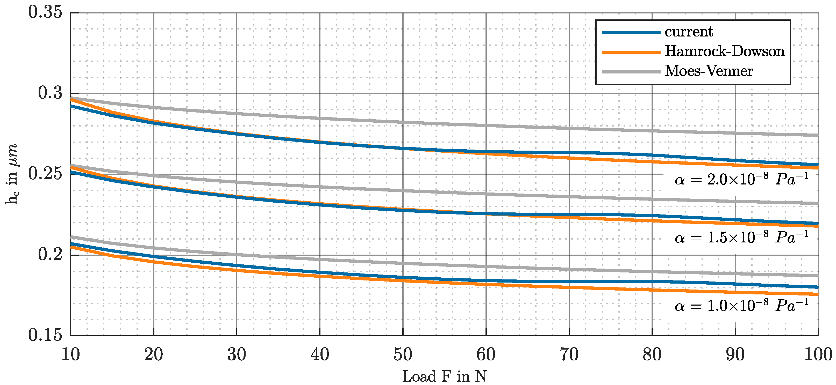
In Figure 5, the results for the central film thickness in the smooth case are compared with the results of Hamrock–Dowson and Moes–Venner [2].

5.5. Results for the Rough Case

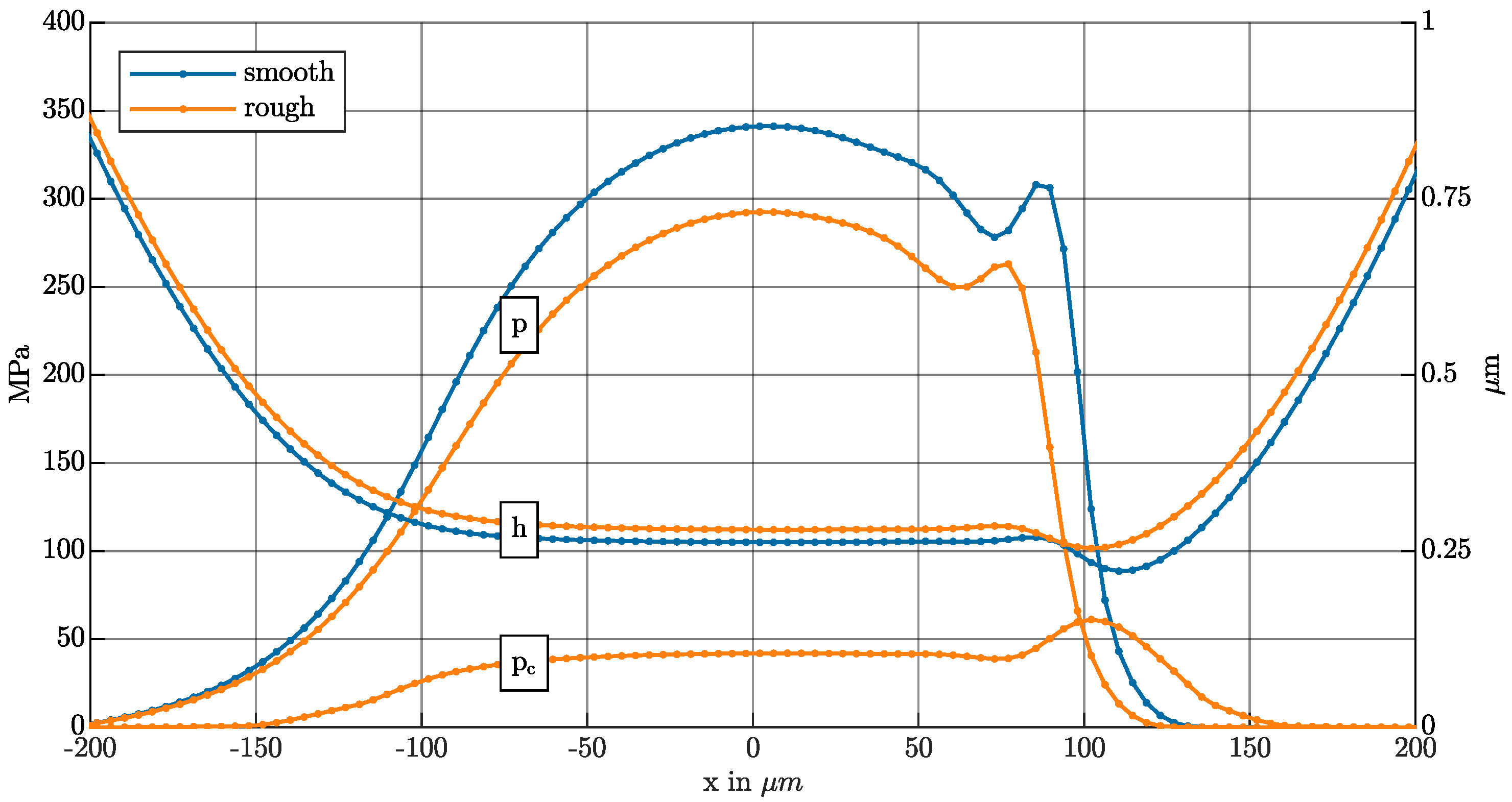
In Figure 6, the results for both cases are compared. Due to the solid body contact pressure, the hydrodynamic pressure is lower in the rough case, as shown in Figure 7. The total pressure is also lower. The minimum gap height is higher.
As a further test, the results of our model were compared with the results published by Khonsari [9]. The results for a dimensionless central film thickness H c = h c / R x , a dimensionless minimum film thickness H m i n = h m i n / R x , and an asperity–load aspect ratio L a are shown in Table 3. The fixed input parameters are R x = 13 mm, U 1 = U 2 = 6.2 m/s, E = 226 GPa, η 0 = 0.03 Pa·s, and α = 2 · 10 8 m2/N. The other parameters are determined to satisfy the dimensionless numbers κ = a / b , W = F E R x 2 , U = η 0 ( U 1 + U 2 ) 2 E R x , G = α E , and σ ¯ = R q / R x , whereby the roughness was scaled in our model. Khonsari treated the roughness differently, which limits the comparability. However, the predictions of both models agree well for the operating points analyzed, although our model predicts slightly lower values for the film thickness.

6. Convergence and Solution Time

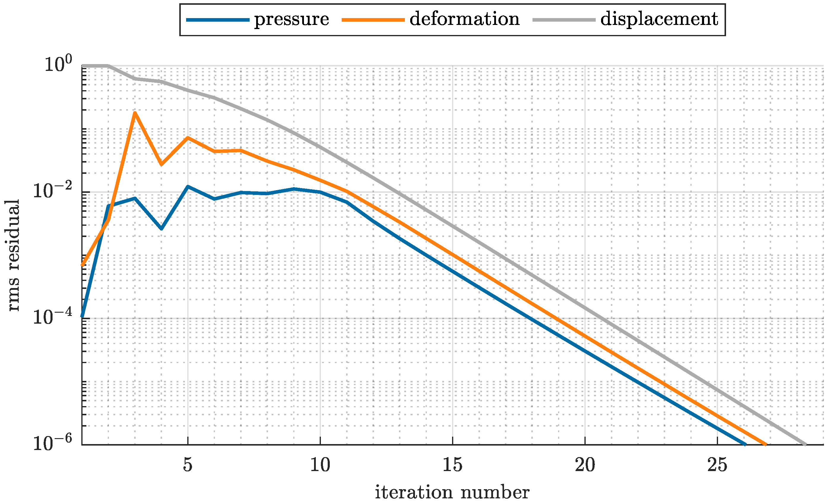
To monitor the solution process and to obtain a convergence criterion, the raw residuals are normalized. In Figure 8, the RMS residuals for each set of equations are displayed over the iteration number for n = m = 40 . The convergence criterion is 10 6 .
To demonstrate the number of iterations and the solution time required for the model, we performed a test with our implementation and using an Intel Xeon W-2123 CPU, the results of which are shown in Table 4.
The convergence and solution time of our approach can be compared with the solution method of Gu [11], which used a similar model with an iterative strategy. Gu gives a number of iterations between 56 and 210 for a smooth case and between 231 and 941 for a rough case. For the solution time, he gives a value between 2.86 and 9.58 s for the smooth case and between 11.16 and 39.17 for the rough case but without specifying the mesh size used. The convergence of our approach can also be compared, with restrictions, with the approach of Habchi [5], which also coupled pressure and deformation but determined h 0 in an outer iteration loop and applied a deformation equation for a 3D structure. Habchi gives a total number of iterations from 10 to 100 depending on the initialization but without giving a convergence criterion. For the computation time, he gives 2.875 to 50.281 seconds per iteration.

7. Conclusions

In this paper, a new scheme for the implicit treatment of general mixed EHL problems was presented. The method developed has been validated and shown to be accurate and robust. Our fully implicit method offers significant advantages in terms of computational efficiency and stability. The use of co-allocated grids reduces the complexity of the implementation and the computational effort. The resulting linear equation system can be efficiently solved by Krylov subspace methods. By implementing our method in a computational program, an almost arbitrary EHD problem can be solved by a user. This is an enrichment of many applications in mechanical engineering and medical technology. The current implementation already has a good solution time and a lower number of iterations compared to similar models. Further improvements in speed can be expected with optimized code in a machine-oriented language. In summary, it can be said that this fully implicit coupled scheme represents a significant advance in numerical tribology.

Author Contributions

Conceptualization, methodology, software, validation, investigation, writing—original draft preparation, and visualization, S.W.; writing—review and editing, H.S. and S.W.; supervision, H.S. All authors have read and agreed to the published version of the manuscript.

Funding

This research received no external funding.

Data Availability Statement

The original contributions presented in the study are included in the article, further inquiries can be directed to the corresponding authors.

Conflicts of Interest

The authors declare no conflicts of interest.

Nomenclature

Latin symbols
a , b radii of the Hertzian contact ellipse
dcoefficient of the pressure correction term
d H deformation of the Hertzian contact ellipse
E 1 , E 2 Young’s modulus of body 1, 2
E reduced Young’s modulus
hfilm thickness
welastic deformation
h c central film thickness
h 0 rigid body displacement
J Jacobian
Kdeformation kernel
n normal vector
phydrodynamic pressure
p a atmospheric pressure
p c contact pressure
p 0 ref. pressure in Roelands’ equation
R x , R y auxiliary radii
R 1 x , R 2 x radii of body 1, 2 along x
R 1 y , R 2 y radii of body 1, 2 along y
U 1 , U 2 surface velocity
Xgeneral solution variable
x , y spatial coordinates
zexponent in Roelands’ equation
Greek symbols
α pressure–viscosity coefficient
β explicit under-relaxation factor
α B Bunsen solubility coefficient
θ fractional film content
λ empirical factor of pressure correction term
ν 1 , ν 2 Poisson’s ratio of body 1, 2
ρ fluid density
ρ 0 density at atmospheric pressure
Φ p tensor of pressure flow factors
Φ p x , Φ p y pressure flow factors
Φ s tensor of shear flow factors
Φ s x , Φ s y shear flow factors
η dyn. viscosity
η 0 viscosity at atmospheric pressure
ω implicit under-relaxation factor
Ω integration domain
Ω boundary of Ω

Appendix A. Accuracy of the Pressure Gradient Approximation

Assuming that the pressure varies as a second-order polynomial along x as follows
p ( x ) = a ( x x P ) 2 + b ( x x P ) + c
the pressure at the neighbor nodes becomes
p W W = 4 a Δ x 2 2 b Δ x + c p W = a Δ x 2 b Δ x + c p P = c p E = a Δ x 2 + b Δ x + c p E E = 4 a Δ x 2 + 2 b Δ x + c
As a result, correction term (16) becomes
3 2 p P p W p E + 1 4 p W W + 1 4 p E E = 3 2 c ( a Δ x 2 b Δ x + c ) ( a Δ x 2 + b Δ x + c ) + 1 4 ( 4 a Δ x 2 2 b Δ x + c ) + 1 4 ( 4 a Δ x 2 + 2 b Δ x + c ) = a Δ x 2 1 1 + 4 4 + 4 4 + b Δ x 1 1 2 4 + 2 4 + c 3 2 1 1 + 1 4 + 1 4 = 0
This can be applied analogously to each pair of opposite faces, and so the integral of the correction term vanishes for any closed boundary if the pressure varies as a second-order polynomial in space.

References

  1. Hamrock, B.J.; Dowson, D. Isothermal Elastohydrodynamic Lubrication of Point Contacts: Part III—Fully Flooded Results. J. Lubr. Technol. 1977, 99, 264–275. [Google Scholar] [CrossRef]
  2. Venner, C.H.; Lubrecht, A.A. Multilevel Methods in Lubrication; Elsevier: Amsterdam, The Netherlands, 2000. [Google Scholar]
  3. Hughes, T.; Elcoate, C.; Evans, H. Coupled solution of the elastohydrodynamic line contact problem using a differential deflection method. Proc. Inst. Mech. Eng. Part-J. Mech. Eng. Sci. 2000, 214, 585–598. [Google Scholar] [CrossRef]
  4. Zhu, D.; Hu, Y.Z. A Computer Program Package for the Prediction of EHL and Mixed Lubrication Characteristics, Friction, Subsurface Stresses and Flash Temperatures Based on Measured 3-D Surface Roughness. Tribol. Trans. 2001, 44, 383–390. [Google Scholar] [CrossRef]
  5. Habchi, W.; Eyheramendy, D.; Vergne, P.; Morales-Espejel, G.E. A Full-System Approach of the Elastohydrodynamic Line/Point Contact Problem. ASME J. Tribol. 2008, 130, 021501. [Google Scholar] [CrossRef]
  6. Brooks, A.N.; Hughes, T.J.R. Streamline upwind/Petrov-Galerkin formulations for convection dominated flows with particular emphasis on the incompressible Navier-Stokes equations. Comput. Methods Appl. Mech. Eng. 1982, 32, 199–259. [Google Scholar] [CrossRef]
  7. Hajishafiee, A.; Kadiric, A.; Ioannides, S.; Dini, D. A coupled finite-volume CFD solver for two-dimensional elasto-hydrodynamic lubrication problems with particular application to rolling element bearings. Tribol. Int. 2017, 109, 258–273. [Google Scholar] [CrossRef]
  8. Schmidt, J.H. An Efficient Solution Procedure for Elastohydrodynamic Contact Problems Considering Structural Dynamics; KIT Scientific Publishing: Karlsruhe, Germany, 2019. [Google Scholar]
  9. Masjedi, M.; Khonsari, M. On the Effect of Surface Roughness in Point-Contact EHL: Formulas for Film Thickness and Asperity Load. Tribol. Int. 2015, 82, 228–244. [Google Scholar] [CrossRef]
  10. Zhu, D.; Cheng, H. Effect of Surface Roughness on the Point Contact EHL. J. Tribol. 1988, 110, 32–37. [Google Scholar] [CrossRef]
  11. Gu, C.; Zhang, D.; Jiang, X.; Meng, X.; Wang, S.; Ju, P.; Liu, J. Mixed EHL Problems: An Efficient Solution to the Fluid–Solid Coupling Problem with Consideration of Elastic Deformation and Cavitation. Lubricants 2022, 10, 311. [Google Scholar] [CrossRef]
  12. Patir, N.; Cheng, H.S. An Average Flow Model for Determining Effects of Three-Dimensional Roughness on Partial Hydrodynamic Lubrication. J. Lubr. Technol. 1978, 100, 12–17. [Google Scholar] [CrossRef]
  13. Letalleur, N.; Plouraboué, F.; Prat, M. Average Flow Model of Rough Surface Lubrication: Flow Factors for Sinusoidal Surfaces. J. Tribol. 2002, 124, 539–546. [Google Scholar] [CrossRef]
  14. Dowson, D.; Higginson, G.R. Elasto-Hydrodynamic Lubrication: The Fundamentals of Roller and Gear Lubrication; Pergamon Press: London, UK, 1966. [Google Scholar]
  15. Wu, S.R. A penalty formulation and numerical approximation of the Reynolds-Hertz problem of elastohydrodynamic lubrication. Int. J. Eng. Sci. 1986, 24, 1001–1013. [Google Scholar] [CrossRef]
  16. Elrod, H.G. Titel. J. Lubr. Technol. 1981, 103, 350–354. [Google Scholar] [CrossRef]
  17. Bair, S. The high pressure rheology of some simple model hydrocarbons. Proc. Inst. Mech. Eng. Part J. Eng. Tribol. 2002, 216, 139–149. [Google Scholar] [CrossRef]
  18. Roelands, C.J.A. Correlational Aspects of the Viscosity-Temperature-Pressure Relationship of Lubricating Oils. Doctoral Thesis, Technical University of Delft, Delft, The Netherlands, 1966. [Google Scholar]
  19. Ferziger, J.H.; Peric, M. Numerische Strömungsmechanik; Springer: Berlin/Heidelberg, Germany, 2008. [Google Scholar]
  20. Boresi, A.P.; Schmidt, R.J. Advanced Mechanics of Materials, 5th ed.; John Wiley & Sons: Hoboken, NJ, USA, 1993. [Google Scholar]
  21. Saad, Y. Iterative Methods for Sparse Linear Systems; Society for Industrial and Applied Mathematics: Philadelphia, PA, USA, 2003. [Google Scholar]
  22. Findeisen, D.; Helduser, S. Ölhydraulik; (6.Auflage); Springer: Berlin/Heidelberg, Germany, 2014. [Google Scholar]
  23. Hu, Y.Z.; Tonder, K. Simulation of 3-D random rough surface by 2-D digital filter and fourier analysis. Int. J. Mach. Tools Manuf. 1992, 32, 83–90. [Google Scholar] [CrossRef]
  24. Arthur, F.; Noël, B. A hybrid method for fast and efficient rough surface generation. Proc. Inst. Mech. Eng. Part J. Eng. Tribol. 2015, 230, 747–768. [Google Scholar]
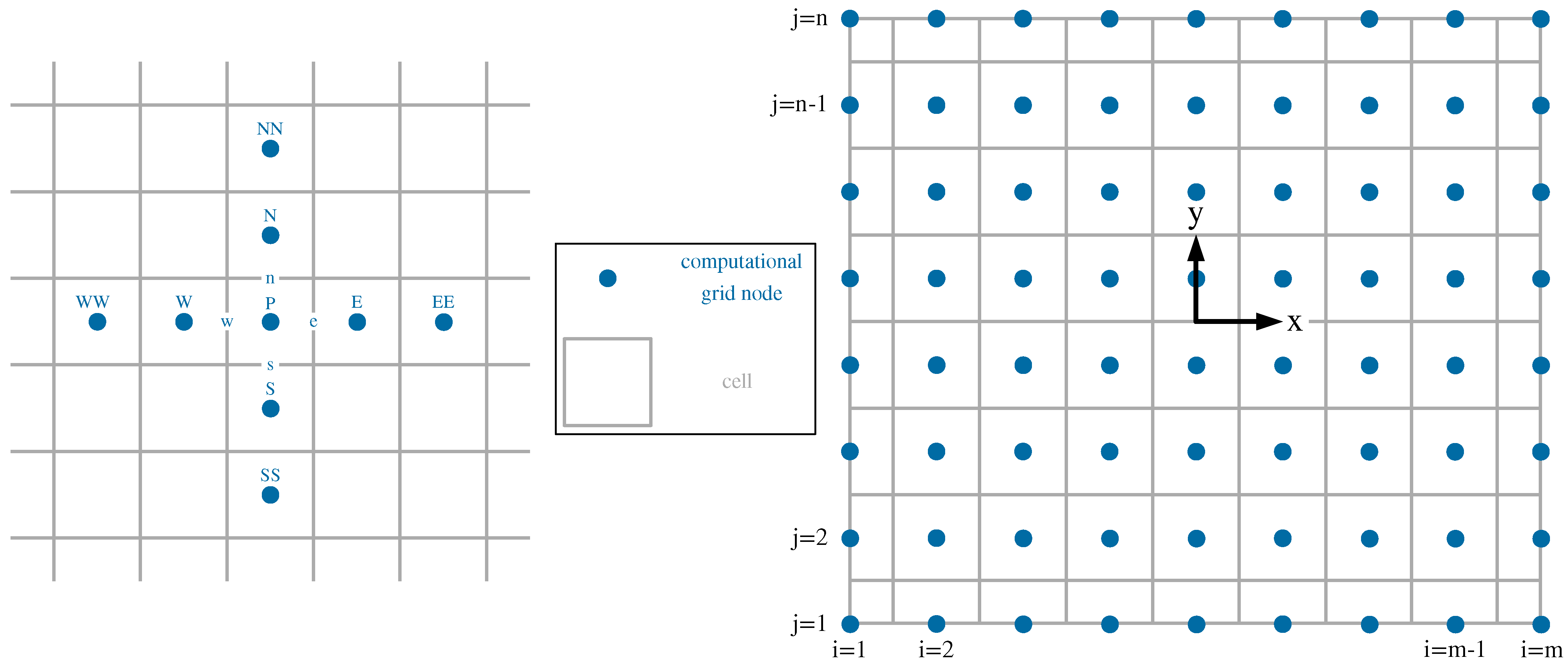
Figure 1. Spatial discretization on a co-allocated Cartesian grid.
Lubricants 12 00322 g001
Figure 2. Sparsity pattern for a 8 × 8 grid: (a) smooth case; (b) rough case.
Lubricants 12 00322 g002
Figure 3. (a) Surface height distribution of the generated surface; (b) flow factors and contact pressure for the rough case.
Lubricants 12 00322 g003
Figure 4. Mesh study for the smooth case: (a) pressure; (b) minimum fill thickness; (c) maximum pressure.
Lubricants 12 00322 g004
Figure 5. Central film thickness for various loads and viscosity–pressure coefficient combinations.
Lubricants 12 00322 g005
Figure 6. Rough case results: (a) hydrodynamic pressure; (b) contact pressure; (c) gap height.
Lubricants 12 00322 g006
Figure 7. Comparison of pressure and gap height for smooth and rough cases along x.
Lubricants 12 00322 g007
Figure 8. Convergence history for the smooth test case.
Lubricants 12 00322 g008
Table 1. Values of the parameters for the test case.
ParameterValueUnitParameterValueUnit
E 2.26 × 10 11 N/m2 α 2.2 × 10 8 m2/N
F 10 100 N α B 0.09 [22]1
L x / a = L y / b 41 η 0 40 × 10 3 N s/m2
R x = R y 16 × 10 3 m ρ 0 853kg/m3
U 1 = U 2 0.8 m/s
Table 2. Values for pressure flow factor, shear flow factor, and contact pressure.
h ¯ in μm Φ p Φ s p ¯ c in MPa
0.16260.0142−0.5397159.0373
0.17690.0583−0.4005133.2646
0.21150.2616−0.212387.8586
0.25450.5316−0.084649.5630
0.31170.7519−0.014422.5594
0.38590.87520.01058.5413
0.56260.95640.01190.0771
0.74990.97460.00680
0.93740.98330.00430
1.12490.98820.00300
1.31240.99120.00220
Table 3. Comparison of the results for the rough case using the current model (left) with those of Khonsari [9] (right).
κ WUG σ ¯ 10 5 · H c H m i n L a
1 1 × 10 6 1 × 10 11 4972 2 × 10 5 1.8 1.58 2.17 2.13 34 34.7
2 1 × 10 6 1 × 10 11 4972 2 × 10 5 2.04 2.15 2.35 2.51 31.2 31.9
3 1 × 10 6 1 × 10 11 4972 2 × 10 5 2.18 2.37 2.44 2.63 29.9 32.5
4 1 × 10 6 1 × 10 11 4972 2 × 10 5 2.28 2.43 2.5 2.74 29.3 34.1
6 1 × 10 6 1 × 10 11 4972 2 × 10 5 2.39 2.52 2.58 2.86 29.1 35.8
8 1 × 10 6 1 × 10 11 4972 2 × 10 5 2.42 2.58 2.63 2.93 29.4 37.7
Table 4. Iteration numbers and CPU time for the test cases.
nNumber of IterationsSolution TimeTime per Iteration
SmoothRoughSmoothRoughSmoothRough
1031300.923551.8480.0297920.061601
1532322.28885.22060.0715260.16314
2031305.815915.0330.187610.50111
25293011.05629.9990.381250.99998
30293021.2867.1310.733782.2377
35293036.181123.411.24764.1136
40293060.634227.512.09087.5836
45293091.972414.363.171413.812
502930142.6730.074.917324.336
553430231.81213.46.817840.446
606330595.411918.19.450963.935
Disclaimer/Publisher’s Note: The statements, opinions and data contained in all publications are solely those of the individual author(s) and contributor(s) and not of MDPI and/or the editor(s). MDPI and/or the editor(s) disclaim responsibility for any injury to people or property resulting from any ideas, methods, instructions or products referred to in the content.