Abstract
The present study aims to efficiently predict the wear volume of a journal bearing under start–stop operating conditions. For this purpose, the wear data generated with coupled mixed-elasto-hydrodynamic lubrication (mixed-EHL) and a wear simulation model of a journal bearing are used to develop a neural network (NN)-based surrogate model that is able to predict the wear volume based on the operational parameters. The suitability of different time series forecasting NN architectures, such as Long Short-Term Memory (LSTM), Gated Recurrent Unit (GRU), and Nonlinear Autoregressive with Exogenous Inputs (NARX), is studied. The highest accuracy is achieved using the NARX network architectures.
1. Introduction
Preventing wear-induced failures of machines is one important measure to become more sustainable and reduce CO2 emissions, as maintenance and replacement efforts due to wear-induced failures share about 3% of global primary energy consumption [1]. Journal bearings are regarded as one wear-critical component in a machine. Hydrodynamic journal bearings can operate free of wear during nominal operation, but they are prone to abrasive wear during start–stop operation [2,3,4]. Advancing wear losses can lead to a loss of conformity, which may cause irregular vibrations or even a loss of load-carrying capacity. The latter can cause severe consequential damage to the machine. Therefore, potential methods to predict the wear of a journal bearing during mixed-friction operation are needed. Various studies have tackled the damage caused by mixed-friction operation, and promising physical approaches have been developed and validated [2,5,6]. These models can provide accurate results if the operating conditions of a specific machine in terms of load, speeds, and temperature as well as the physical properties of the specific bearing material–lubricant combinations are predefined. However, in many cases, these numerical approaches are still very time-consuming, making their effective utilization in design and direct integration into condition monitoring impractical.
In recent years, in the age of artificial intelligence (AI) and machine learning (ML), so-called surrogate or meta models have been developed in the field of tribology [7,8]. These models can replace computationally expensive physical and empirical models for different purposes, including wear prediction [9,10,11]. After successful training, these models can predict the desired output with high accuracy within much shorter calculation times than the original physical simulation approaches. Hence, ML-based models can handle a large variety of operating conditions and parameters in real time or near real time. This capability allows for predicting wear under dynamic conditions, such as start–stop conditions with sequential mixed-friction operation, which are often observed in real machinery. From a practical point of view, ML-based models of tribological systems can be applied in the design and the use phases of these systems. Specifically, the designer can use ML-based models to efficiently assess the impact of the design as well as operational conditions on wear. In the use phase, wear monitoring can benefit from a correlation between sensor data, i.e., measurable bearing condition indicators, and the corresponding wear losses, which can typically not be directly measured.
The focus of this study is use phase wear monitoring. For this purpose, it is hypothesized that the knowledge gained through experimentally validated physical simulation methods and the sensor data obtained through condition monitoring with tribology-related signals in the real system, e.g., temperature, load, torque, or Acoustic Emission, are complementary and can be used to develop novel methods for accurate and robust ML-based wear monitoring during the use phase of a particular machine.
As a first step towards this vision, the aim of this study is to evaluate the capabilities of ML for the prediction of wear in journal bearings under start–stop conditions. For this purpose, the wear data obtained with an existing, experimentally validated coupled mixed-elasto-hydrodynamic (mixed-EHL) and wear simulation model are used to train and evaluate an ML-based surrogate model. Three similar start–stop cycles in terms of time and speed with different bearing loads and temperatures serve as the input, whereas the corresponding wear volume serves as the output.
2. Methods and Parameters
The methodology of this work is shown in Figure 1. Firstly, the mixed-EHL and wear simulation model was used to generate wear data. Following the pre-processing of the generated data, multiple variants of the three time series forecasting recurrent neural network (RNN) architectures, namely Long Short-Term Memory (LSTM), Gated Recurrent Unit (GRU), and Nonlinear Autoregressive with Exogenous Inputs (NARX), were built. The aim was to explore the suitability of the chosen architectures as well as the impact of the number of hidden layers (HL) and neurons per layer on the prediction accuracy. To compare RNN architectures, each network architecture was simulated using the same training and test data sets. At the beginning of the training, the weights and biases of the neural network must be set to specific initial values. The initial determination of the values is called the “initial guess”. The training algorithm does this by means of random initialization. As the choice of initial values for weights and biases influences the training, the training was repeated several times, and the best result was saved. Subsequently, the aim was to elucidate whether the best-performing RNN can predict wear if the sampling rate of the data sets is reduced. The reason for this is twofold. On the one hand, training with large data sets is computationally expensive and time-consuming. By using lower sampling rates, not only can the time be reduced but also the necessary hardware costs. On the other hand, the acceleration and deacceleration rates as well as the operating time of dynamically operating machines may vary, which affects the number of sampling points in a whole cycle and thereby the seasonality of the data. From a data science point of view, this different seasonality of the data can also be achieved by varying the sampling rate of the data sets, as it is conducted in this study. It should be noted that the stochastic operation is far more complex in terms of loads, speeds, and temperatures. Hence, this can only be seen as a first step towards wear prediction under dynamic conditions. In this study, the best-performing model architecture from our initial screening of LSTM, GRU, and NARX was trained again using training data with different sampling rates. Specifically, the sample rate of the training data was heuristically changed by a downsampling factor of 50, 100, and 400 using the function downsample within MATLAB. The downsampling factor determines the data points that are maintained from the original training data. With a downsampling factor of 50, only every 50th value is maintained. Subsequently, the model was tested with testing data at a downsampling factor of 200 to obtain a first idea of the model’s adaptability to condition-monitoring systems with lower sampling rates as well as dynamic operating conditions.
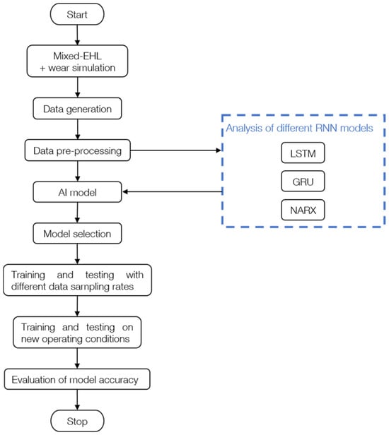
Figure 1.
Process chart depicting the methodology of the present work.
Finally, the best-performing RNN model from our initial screening was trained on series A and B and then tested on series C to show the transferability of the model to different operational conditions.
2.1. Coupled Mixed-EHL and Wear Simulation Model
In this study, a coupled transient mixed-elasto-hydrodynamic (mixed-EHL) and wear simulation model is used to simulate the wear behavior during multiple thousand start–stop cycles. The basic structure of the physical simulation model and its combination with a wear simulation with empirical wear laws is shown in Figure 2.
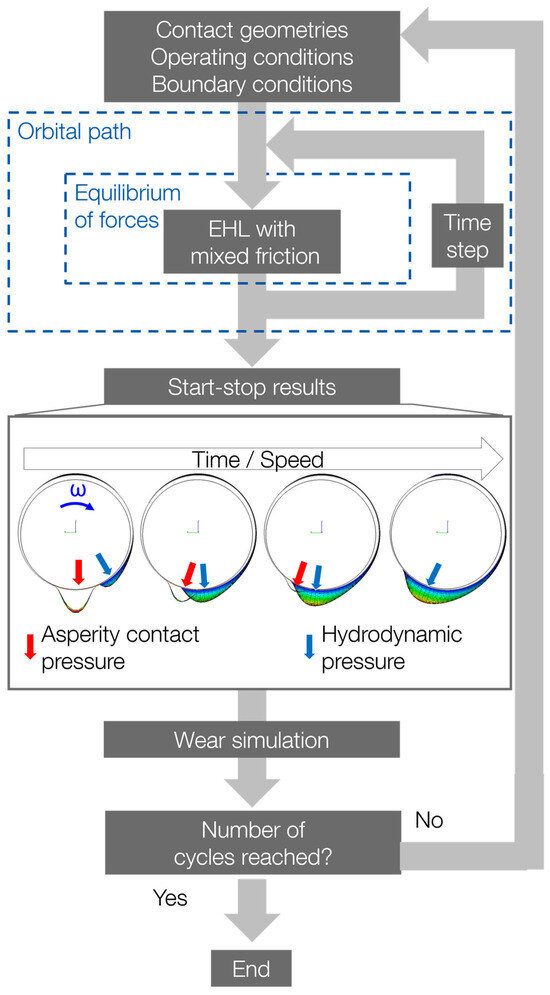
Figure 2.
Structure of the mixed-EHL and wear simulation.
In this model, which is built in AVL Excite PowerUnit, the initial contact geometry, the surface topography of the bearing and shaft, and the transient operating conditions are used as input parameters. Furthermore, the temperature, boundary friction, and wear coefficient are used as inputs. The variation in temperature affects the lubricant’s viscosity and therefore the hydrodynamic film formation. The relationship between temperature, pressure, and lubricant viscosity, which was used in this study, is shown in Figure A1 in Appendix A. The friction coefficient was modeled with the boundary friction model according to Knauss and Offner [12]. Changing the lubricant type, the base oil viscosity, and the additives will certainly have an influence on the friction coefficient.
In transient mixed-elasto-hydrodynamic simulations (EHL with mixed friction), the local, transient wear-critical pressures are calculated. After each simulation step, which corresponds to one start–stop cycle, the wear pattern is calculated using the energetic approach according to Fleischer [13,14], which calculates the local wear depth as a function of the locally resolved coefficient of friction (CoF), the asperity contact pressure, as well as a predefined wear coefficient. Subsequently, the maximum wear per simulation step is extrapolated to 0.25 µm for the maximum wear depth to calculate the wear loss caused by multiple start–stop cycles within one simulation step. In the next step, the wear volume is calculated via integration. After the wear calculation, a new simulation model is built with an updated contour and bearing roughness. This process is repeated with updated wear profiles and surface topographies of the bearing in each simulation step until a predefined simulation time is reached.
2.2. Data Generation from the Simulation Model
The coupled, transient mixed-EHL + wear simulation model can be used to predict the contact conditions inside of the journal bearing as well as volumetric wear losses for different operational conditions, i.e., loads, temperatures, and speeds. The data used in this study are from three different start–stop time series, namely series A, B, and C. In all cases, the modeled bearing has a diameter of 30 mm, a width of 15 mm, and a radial clearance of 25 µm. For Series A, a radial load of 900 N and a temperature of 80 °C were chosen, while a load of 900 N and a temperature of 90 °C and a load of 1350 N and a temperature of 80 °C were chosen for series B and C, respectively. With an increase from 80 °C to 90 °C, the base viscosity at 40 °C decreases from 7.2 to 5.7 mPas. In all series, the start–stop cycle is fixed to a 2 s acceleration from 0 to 600 min−1, 2 s at a constant speed for 600 min−1, and a 3 s deceleration from 600 to 0 min−1. Each start–stop cycle lasted 7 s, totaling 45 shaft revolutions per start–stop cycle (10 + 20 + 15 for starting, constant, and stopping mode, respectively). The coupled mixed-EHL + wear simulation was conducted for a total of 2500 start–stop cycles. With 4884 time steps per start–stop cycle, the overall time series contains more than 12 million time steps. The three different load–temperature combinations generate three distinct time series for the simulated contact conditions in the bearing as well as the resulting wear volume.
2.3. Data Pre-Processing
The three distinct data sets for series A, B, and C contain constant input data (load, temperature), transient input data (time, speed), and transient mixed-EHL simulation output data (CoF), alongside the transient output data of the wear simulation (wear volume, wear depth, and wear rate). The input and output variables are referred to as features. From all of these features, a few features were carefully chosen with the idea that only certain measured values are suitable to be measured in real machinery, such as the temperature and speed. The feature temperature was excluded due to the isothermal modeling as a first attempt and could be integrated at a later stage. In contrast, other features, such as the radial bearing load and friction, are difficult to measure and therefore commonly not available. The bearing load can be assumed from the overall torque or energy consumption of a machine. In this study, the radial bearing load remained constant within each simulation run, so it was also excluded from the model [15]. Friction cannot be measured directly, but it is an important parameter. Hence, various studies have shown that friction phenomena can instead be measured with Acoustic Emission technology. Because this is not within the scope of this study, the integral friction coefficient (CoF) was used.
However, it should be noted that the temperature and bearing load are implicitly considered. First, variations in the predefined isothermal temperature and the external load impact the oil viscosity due to temperature– and pressure–viscosity relationships, which affect the hydrodynamic film’s load-carrying capacity. Consequently, the ratio between oil and solid contact pressure is affected, influencing the global CoF, which contains both solid body and fluid friction via the integration of local shear stresses. Second, to incorporate the load’s influence, which also remained constant throughout the simulation, frictional torque was used instead of CoF, as it also contains the external load as a variable, as shown in Equation (1),
where r is the radius of the bearing. Hence, the data were significantly reduced to only contain frictional torque and speed as input parameters for the ML models. The wear prediction model needs to anticipate short-term fluctuations, like changes in operational conditions (such as start–stop cycles), termed seasonality, and long-term wear patterns, known as trend. Hence, “wear volume” was chosen as the output feature instead of transient measures like wear rate, as it effectively encapsulates both seasonality and trend aspects.
In the future, the aim is to replace the simulation data with measured data. Using the measured speed, temperature, and friction torque can be the first step to demonstrate the transferability from simulation to reality.
2.4. Machine Learning Models
The transient data obtained from the simulation model can be treated as a time series for ML-based surrogate modeling. Pragmatically speaking, wear monitoring and prognosis are a combination of regression modeling between input and output data and time series forecasting, commonly performed with RNNs, which are used to predict posterior data while considering the previous and current state of the system. RNNs are able to retain past sequential data in memory, making them exceptionally well-suited for tasks involving sequential data, such as time series analysis. Following the pre-processing of the data obtained from mixed EHL and wear simulations, the different RNN architectures LSTM, GRU, and NARX were trained and compared. These architectures are further introduced in Section 2.4.1, Section 2.4.2 and Section 2.4.3.
2.4.1. LSTM
Long Short-Term Memory (LSTM) is an RNN that avoids the vanishing gradient problem, which occurs during the training of long time series. As shown in Figure 3, LSTMs feature a unique architecture comprising an input gate, a forget gate, and an output gate, enabling them to retain and utilize information over extended sequences selectively. The input gate regulates the flow of new inputs (labeled x) into the cell state (labeled c). Conversely, the forget gate determines which information from the previous cell state is discarded, thereby facilitating the preservation of relevant long-term dependencies. Finally, the output gate controls the flow of information from the cell state to the output (labeled y). This gating mechanism allows LSTMs to capture and retain important temporal dependencies, making them particularly interesting for using sequential data [16,17,18].
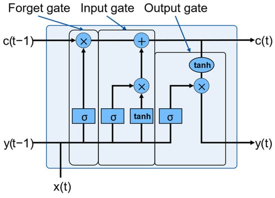
Figure 3.
Schematic representation of the LSTM model.
2.4.2. GRU
Gated Recurrent Unit (GRU) networks are a specialized variant of RNNs, similar to LSTM networks, designed to overcome the vanishing gradient problem inherent in traditional RNN architectures. Compared to LSTMs, GRUs employ a simpler architecture, featuring fewer gating mechanisms while maintaining competitive performance [17]. Within the GRU architecture, depicted in Figure 4, two primary gates regulate the flow of information: the update gate and the reset gate. The update gate in GRUs governs the flow of new inputs (labeled x) into the current state (labeled c), deciding how much past information to retain and how much new information to integrate. Similarly, the reset gate adjusts the contribution of past information when computing the current state, facilitating selective forgetting of irrelevant information. GRU models dynamically adjust these gates to capture and retain relevant information over extended sequences. Compared to LSTMs, GRUs are easier to train and faster to execute at the cost of modeling accuracy [19,20].
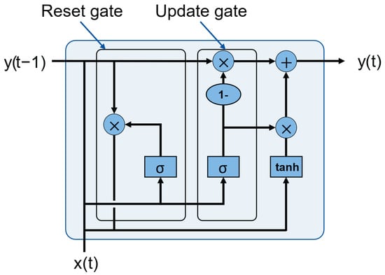
Figure 4.
Schematic representation of the GRU model.
2.4.3. NARX
NARX models, or Nonlinear Autoregressive models with exogenous inputs, are specialized tools for time series forecasting. NARX models capture complex patterns and dynamics due to their capability to integrate speed and frictional torque as input signals into the forecasting process. Unlike traditional autoregressive models, NARX models incorporate exogenous inputs alongside the autoregressive terms, allowing them to account for external influences on the system’s behavior [21,22,23,24,25].
The NARX model equation is shown in Equation (2), where y(t), the predicted value of the model, is predicted using its previous values, y(t − 1) to y(t − ny), and the corresponding previous values of an input signal, x(t − 1) to x(t − nx). There are two forms of NARX architecture: series-parallel and parallel architecture. The series-parallel NARX architecture was chosen for this study as the availability of the previous values of y(t) makes the network more accurate [26].
Here y(t) is the wear volume. The Neural Net Time Series App in MATLAB version R2020b was used for training and testing the NARX models. A schematic representation of the NARX network is shown in Figure 5.
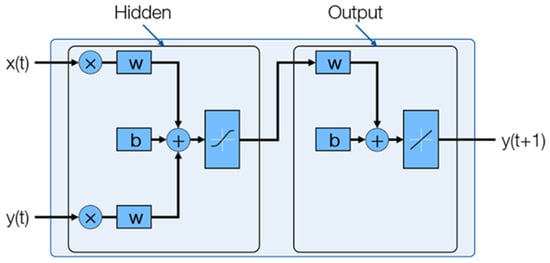
Figure 5.
Schematic representation of the series-parallel NARX model.
3. Results and Discussion
The aim of this project was to train an RNN model that predicts the wear volume data generated from the physics-based simulation model. Three time series, A, B, and C, were generated with different operating conditions, as described in the methods in Section 2.2.
3.1. Mixed-EHL and Wear Simulation Results
The speed and the coefficient of friction (CoF) predicted by the mixed-EHL model for the first three and last three start–stop cycles of series A are exemplarily shown in Figure 6a. It can be observed that the CoF is zero at the initial start-up and stopping time due to standstill. After a certain number of start–stop cycles, the CoF is significantly reduced due to the running in process. During the stationary phase, hydrodynamic lubrication is present, which leads to very low viscous friction losses, as it can be seen in Figure 6b.
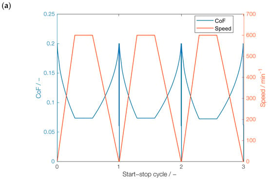
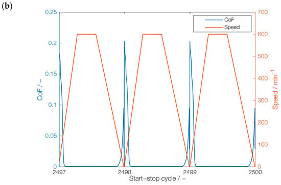
Figure 6.
CoF and speed obtained from physics-based simulation model: (a) cycles 1–3, (b) cycles 2498–2500.
The results of the coupled wear simulation are exemplarily shown in Figure 7. Figure 7a shows the long-term trend of the wear volume. As it can be seen, the wear rate significantly decreases over the number of start–stop cycles after a pronounced wearing-in within the first few hundred start–stop cycles. Turning our attention to the seasonality, the wear volume generated within the first three cycles (1–3) is shown in Figure 7b, while the wear volume originated from the last three cycles (2498–2500) is shown in Figure 7c.
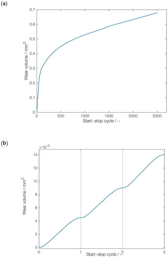
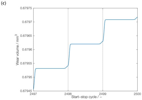
Figure 7.
Wear volume obtained from physics-based simulation model: (a) total number of start–stop cycles, (b) cycles 1–3, (c) cycles 2498–2500.
Similarly to the observed trend, the generated wear volume loss within the first three cycles (0.015 mm3) is significantly higher than the loss within the last three cycles of the data set (0.0003 mm3), as the wear during the first three cycles was generated during the running-in period. In contrast, the wear during the last three cycles was predominantly caused by the mixed-friction operation during start-up and only slightly increased during stopping. The challenge is to incorporate the overall trend and seasonality effects into an efficient, predictive RNN model.
3.2. ML Models and Architecture Comparison
A detailed comparison of LSTM, GRU, and NARX was conducted to evaluate the performance of these RNN architectures for predicting wear in journal bearings during start–stop cycles. The number of layers and the number of neurons per layer were varied for each of the three different RNN architectures to evaluate the performance under various configurations.
The data set was initially downsampled by a downsampling factor of 200 to accelerate convergence during training. An 80–20 data split was used, with 80% allocated to training and 20% reserved for testing. This ratio was chosen based on previous studies. Due to the early pre-screening of these models, the validation data were included for both LSTM and GRU models. Overfitting is prevented by using gradient clipping, limiting the absolute value of the gradients to 1. In the NARX model, the 80% training data set is subdivided, with 60% used for training and 20% as a validation data set. Table A2 and Table A3 in the Appendix A provide detailed information on the training parameter for LSTM, GRU, and NARX. The evaluation was based on the Root Mean Square Error (RMSE) metric for both training as well as testing error analysis. Figure 8 shows the comparison of the three RNN architectures; the complete list of RMSE values can be found in Table A1 in the Appendix A. Variants for each RNN architecture include models with a single hidden layer and two hidden layers for varying numbers of neurons. The test case results for each network are shown in Figure 8. The best results for LSTM were obtained for two hidden layers with 50 neurons in each layer. For GRU, the best results were obtained for a single hidden layer with 100 neurons, whereas for NARX, a single hidden layer with 50 neurons gave the best result. The RMSE value of the NARX model is much lower compared to LSTM and GRU, which can also be observed in the deviations, which are shown in Figure 9. The predictions from LSTM and GRU show local fluctuation, making them unsuitable for prediction of the seasonality. Additionally, the training process of the NARX network was considerably faster than the other two networks. However, due to the uncertain outcome of the comparison between different networks, the training time was not our focus and therefore not measured. Therefore, the NARX model was selected as the most promising model for further training and testing.
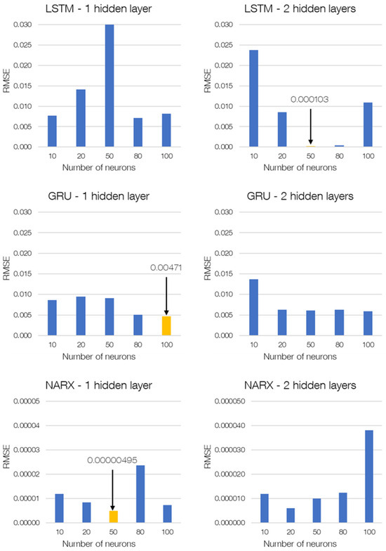
Figure 8.
ML model and architecture comparison for the test case.
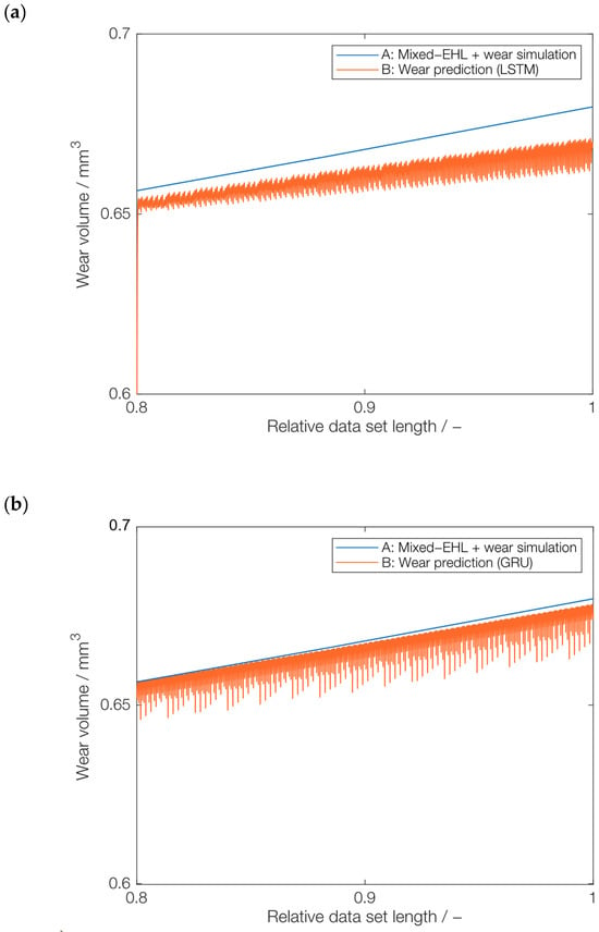
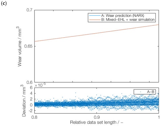
Figure 9.
ML model comparison: (a) LSTM (2 HL, 50 neurons), (b) GRU (1 HL, 100 neurons), and (c) NARX (1 HL, 50 neurons), including deviation from the physics-based wear volume values.
3.3. Exploring the Adaptability of the NARX Model to Varying Data Resolutions
During dynamic operation, the acceleration and deceleration may be subjected to change. Under the assumption of a sampling rate of a condition-monitoring system, this leads to a different number of data points for a given start–stop cycle. The question is whether this change affects the outcome of the model. Therefore, this section focuses on the prediction of multiple downsampled versions of the Series A data set. These downsampled versions were produced by applying downsampling factors of 50, 100, and 400. The NARX model was then trained in three different orders, specifically, 50-400-100, 400-100-50, and 100-50-400. Following the training process, the NARX model with a single hidden layer of 50 neurons was tested on series A with a downsampling factor of 200. The idea to train on different downsampling factors (50, 100, and 400) and to test it on a new downsampling factor of 200 was to artificially check the NARX model’s adaptability to varied sampling rates as well as varied acceleration and deacceleration rates. Although downsampling does not directly influence acceleration and deceleration rates, the concept of the sampling rate offers a parallel understanding: just as a higher sampling rate captures finer details in signal processing, faster changes in velocity signify more rapid acceleration or deceleration. Therefore, if NARX predicts the wear successfully for downsampled data, it is assumed that a similar principle will work for dynamic cycle lengths. The best test results (data set of downsampling factor 200) were achieved with a training sequence of 50-400-100, shown in Figure 10. As it can be seen in Figure 10a, the predicted wear volume of the NARX model is very close to the wear volume of the simulation model. The NARX model was successful in predicting the trend but was unable to capture the local seasonality with high accuracy, as it can be seen in Figure 10b. Even though there are some fluctuations in the prediction, the error is within the range of 0.01.
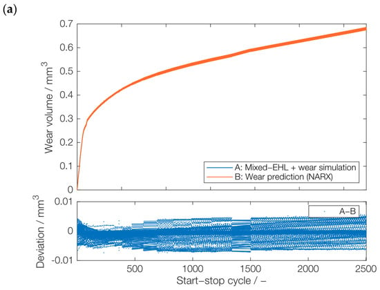
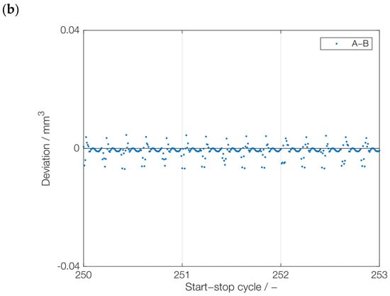
Figure 10.
Prediction of a novel, downsampled series: (a) test results with a downsampling factor of 200 by NARX model trained on downsampling factors of 50, 400, and 100, and (b) deviations from the actual wear volume values (cycles 251–253).
From the comparison between the best test results in Figure 10 and the other two results, which are shown in Appendix A, Figure A2 and Figure A3, it can be observed that both the sequential training with 50-400-100 (Figure 10) and 100-50-400 (Figure A3) lead to comparable results, with a slightly better prognosis result using 50-400-100. In contrast, the sequential training 400-50-100 (Figure A2) leads to larger deviations, particularly after multiple hundred start–stop cycles. One potential reason is that the initial training of NARX with a downsampling factor of 400 can lead to a wrong direction of weights and biases, which ultimately affects the results. This would agree with the results for 50-400-100 (Figure 10) and 100-50-400 (Figure A3), which leads to slightly better results when finishing the training with a downsampling factor of 100 instead of 400. Based on these results, it can be assumed that the downsampling factor of 400 is not beneficial for training, which should be further studied in the future. Nevertheless, based on the positive results with 50-400-100 (Figure 10) and 100-50-400 (Figure A3), the NARX model can be suitable for wear trend prediction under varying dynamic conditions and sampling rates. The suitability of NARX in terms of seasonality is also demonstrated by the minor deviations between its wear prediction and the physics-based wear simulation.
3.4. Utilizing the Trained NARX Model for Forecasting a Novel Series under New Operating Conditions
The NARX model with a single hidden layer of 50 neurons underwent training using two distinct series from the data sets Series A and Series B, featuring loads of 900 N and temperatures of 80 °C and 90 °C, respectively. The training incorporated different downsampling factors, specifically 50 and 100. Afterwards, the trained NARX model was tested with an entirely new series, Series C, without downsampling. In this case, low RMSE values were observed (0.000571). As it can be seen from Figure 11a, the prediction curve is almost identical to the wear volume curve obtained in physics-based simulations. The deviations between NARX and the coupled mixed-EHL and wear simulation are within 0.005, as shown in Figure 11b. This underscores NARX’s remarkable predictive capability in accurately forecasting unknown time series data, highlighting its potential for predictive maintenance applications in dynamic systems.
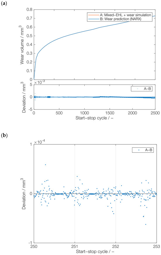
Figure 11.
Prediction of series C (no downsampling): (a) wear volume by the NARX model for the test case trained on series A and B and (b) deviations from the actual wear volume values (cycles 251–253).
4. Conclusions
Journal bearings’ start–stop operation increases the risk of failure due to abrasive wear. Considering the high computational cost of mixed-EHL and wear simulations to predict abrasive wear under dynamic conditions, this work aimed to study the potential of machine learning with recurrent neural networks (NNs) to predict wear after 2500 start–stop cycles.
Based on the results of this work, the following conclusions can be drawn:
- The NARX model exhibited superior predictive performance in wear prediction compared to the LSTM and GRU models, showcasing a lower RMSE.
- The trained NARX model demonstrated robust predictive capabilities, accurately forecasting all time series, irrespective of varying downsampling requirements, underscoring its adaptivity and generalization ability.
- The NARX’s demonstrated effectiveness across diverse scenarios highlights its potential utility in various applications, accentuating its generalization capabilities to handle varying input parameters and data configurations.
Following the original hypothesis, the knowledge gained through experimentally validated physical simulation methods can be used for accurate and robust ML-based wear monitoring. In the future, the input data should be replaced by sensor data obtained through condition monitoring with tribology-related signals in the real system, e.g., temperature, torque, vibration, or Acoustic Emission [3,27]. Furthermore, for the condition monitoring of dynamic operating machinery under real-life, stochastic conditions, which was originally formulated within the hypothesis, this work should be extended towards more complex load cases in terms of speed profiles, temperatures, and loads. In addition, the deviations between the surrogate model and the real data from the experiment should be incorporated using statistical methods [28]. Furthermore, different failure modes should be addressed in the future by applying ML for classification [29].
Author Contributions
Conceptualization, F.K.; methodology, F.K. and A.S.; software, F.K., A.S. and F.W.; validation, F.K., A.S. and F.W.; formal analysis, F.W. and A.S.; investigation, F.K., A.S. and F.W., resources, G.J.; data curation, F.K., A.S. and F.W.; writing—original draft preparation, F.K., A.S. and F.W.; writing—review and editing, F.K., F.W. and G.J.; visualization, F.K. and F.W.; supervision, F.K.; project administration, F.K.; funding acquisition, F.K. All authors have read and agreed to the published version of the manuscript.
Funding
Funded by the Federal Ministry of Education and Research (BMBF) and the Ministry of Culture and Science of the German State of North Rhine-Westphalia (MKW) under the Excellence Strategy of the Federal Government and the Länder.
Data Availability Statement
The data sets presented in this article are not readily available because the data are part of an ongoing study. Requests to access the data sets should be directed to F.K.
Acknowledgments
F.K. acknowledges the funding provided within the RWTH ERS SeedFund start-up project ‘beArIngs’.
Conflicts of Interest
The authors declare no conflicts of interest.
Appendix A

Table A1.
Test results of all trained RNN architectures in Section 3. The best-performing RNN of each architecture is highlighted by bold and underscored letters.
Table A1.
Test results of all trained RNN architectures in Section 3. The best-performing RNN of each architecture is highlighted by bold and underscored letters.
| Model | Hidden Layer | Neurons | RMSE-Test |
|---|---|---|---|
| LSTM | 1 | 10 | 7.72 × 10⁻³ |
| LSTM | 1 | 20 | 1.41 × 10⁻² |
| LSTM | 1 | 50 | 2.19 × 10⁻¹ |
| LSTM | 1 | 80 | 7.10 × 10⁻³ |
| LSTM | 1 | 100 | 8.15 × 10⁻³ |
| LSTM | 2 | 10 | 2.38 × 10⁻² |
| LSTM | 2 | 20 | 8.53 × 10⁻³ |
| LSTM | 2 | 50 | 1.03 × 10⁻⁴ |
| LSTM | 2 | 80 | 1.26 × 10⁻⁴ |
| LSTM | 2 | 100 | 1.09 × 10⁻² |
| GRU | 1 | 10 | 8.59 × 10⁻³ |
| GRU | 1 | 20 | 9.45 × 10⁻³ |
| GRU | 1 | 50 | 9.08 × 10⁻³ |
| GRU | 1 | 80 | 5.05 × 10⁻³ |
| GRU | 1 | 100 | 4.71 × 10⁻³ |
| GRU | 2 | 10 | 1.37 × 10⁻² |
| GRU | 2 | 20 | 6.25 × 10⁻³ |
| GRU | 2 | 50 | 6.11 × 10⁻³ |
| GRU | 2 | 80 | 6.26 × 10⁻³ |
| GRU | 2 | 100 | 5.91 × 10⁻³ |
| NARX | 1 | 10 | 1.20 × 10⁻⁵ |
| NARX | 1 | 20 | 8.51 × 10⁻⁶ |
| NARX | 1 | 50 | 4.95 × 10⁻⁶ |
| NARX | 1 | 80 | 2.37 × 10⁻⁵ |
| NARX | 1 | 100 | 7.33 × 10⁻⁶ |
| NARX | 2 | 10 | 1.20 × 10⁻⁵ |
| NARX | 2 | 20 | 6.07 × 10⁻⁶ |
| NARX | 2 | 50 | 1.00 × 10⁻⁵ |
| NARX | 2 | 80 | 1.25 × 10⁻⁵ |
| NARX | 2 | 100 | 3.82 × 10⁻⁵ |
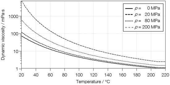
Figure A1.
Relationship between temperature, pressure, and lubricant viscosity.
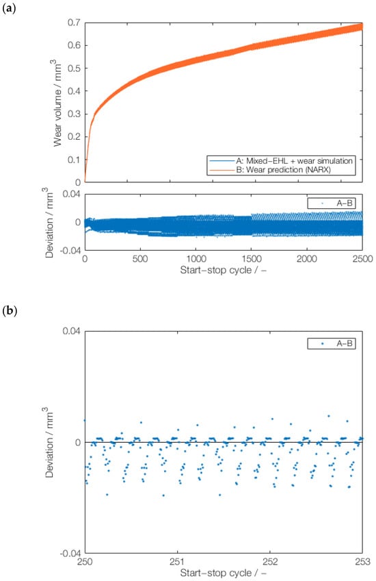
Figure A2.
Prediction of a novel, downsampled series: (a) test results with a downsampling factor of 200 by NARX model trained on downsampling factors of 400, 100, and 50, and (b) deviations from the actual wear volume values (cycles 251–253).
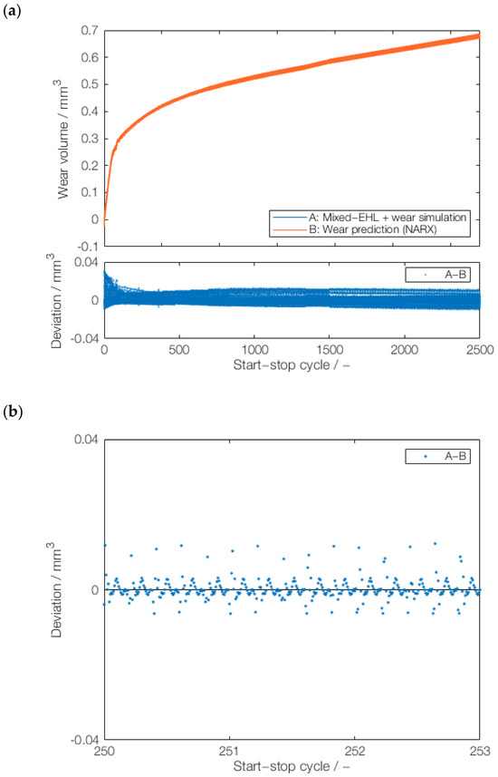
Figure A3.
Prediction of a novel, downsampled series: (a) test results with a downsampling factor of 200 by NARX model trained on downsampling factors of 100, 50, and 400, and (b) deviations from the actual wear volume values (cycles 251–253).

Table A2.
Training parameters of LSTM and GRU.
Table A2.
Training parameters of LSTM and GRU.
| Training Parameter | Description |
|---|---|
| Normalization |
|
| Learning rate |
|
| Optimization methods |
|
| Regularization techniques |
|

Table A3.
Training parameters of NARX.
Table A3.
Training parameters of NARX.
| Training Parameter | Description |
|---|---|
| Normalization |
|
| Learning rate |
|
| Optimization methods |
|
| Regularization techniques |
|
References
- Holmberg, K.; Erdemir, A. Influence of tribology on global energy consumption, costs and emissions. Friction 2017, 5, 263–284. [Google Scholar] [CrossRef]
- König, F.; Chaib, A.O.; Jacobs, G.; Sous, C. A multiscale-approach for wear prediction in journal bearing systems—From wearing-in towards steady-state wear. Wear 2019, 426–427, 1203–1211. [Google Scholar] [CrossRef]
- Zhang, H.; Ma, J.; Li, X.; Xiao, S.; Gu, F.; Ball, A. Fluid-asperity interaction induced random vibration of hydro-dynamic journal bearings towards early fault diagnosis of abrasive wear. Tribol. Int. 2021, 160, 107028. [Google Scholar] [CrossRef]
- Vencl, A.; Rac, A. Diesel engine crankshaft journal bearings failures: Case study. Eng. Fail. Anal. 2014, 44, 217–228. [Google Scholar] [CrossRef]
- Maier, M.; Pusterhofer, M.; Grün, F. Modelling Approaches of Wear-Based Surface Development and Their Experimental Validation. Lubricants 2022, 10, 335. [Google Scholar] [CrossRef]
- Maier, M.; Pusterhofer, M.; Grün, F. Wear simulation in lubricated contacts considering wear-dependent surface topography changes. Mater. Today Proc. 2023, 93, 563–570. [Google Scholar] [CrossRef]
- Marian, M.; Tremmel, S. Current Trends and Applications of Machine Learning in Tribology—A Review. Lubricants 2021, 9, 86. [Google Scholar] [CrossRef]
- Yin, N.; Yang, P.; Liu, S.; Pan, S.; Zhang, Z. AI for tribology: Present and future. Friction 2024, 12, 1060–1097. [Google Scholar] [CrossRef]
- He, Z.; Shi, T.; Xuan, J.; Li, T. Research on tool wear prediction based on temperature signals and deep learning. Wear 2021, 478–479, 203902. [Google Scholar] [CrossRef]
- Bote-Garcia, J.-L.; Gühmann, C. Wear volume estimation for a journal bearing dataset. tm-Tech. Mess. 2022, 89, 534–543. [Google Scholar] [CrossRef]
- Ates, C.; Höfchen, T.; Witt, M.; Koch, R.; Bauer, H.-J. Vibration-Based Wear Condition Estimation of Journal Bearings Using Convolutional Autoencoders. Sensors 2023, 23, 9212. [Google Scholar] [CrossRef] [PubMed]
- Offner, G.; Knaus, O. A Generic Friction Model for Radial Slider Bearing Simulation Considering Elastic and Plastic Deformation. Lubricants 2015, 3, 522–538. [Google Scholar] [CrossRef]
- Fleischer, G. Zur Energetik der Reibung. Wiss. Z. Tech. Univ. Magdebg. 1990, 34, 55–66. [Google Scholar]
- Bartel, D.; Bobach, L.; Illner, T.; Deters, L. Simulating transient wear characteristics of journal bearings subjected to mixed friction. Proc. Inst. Mech. Eng. Part J J. Eng. Tribol. 2012, 226, 1095–1108. [Google Scholar] [CrossRef]
- Moder, J.; Bergmann, P.; Grün, F. Lubrication Regime Classification of Hydrodynamic Journal Bearings by Machine Learning Using Torque Data. Lubricants 2018, 6, 108. [Google Scholar] [CrossRef]
- Lindemann, B.; Müller, T.; Vietz, H.; Jazdi, N.; Weyrich, M. A survey on long short-term memory networks for time series prediction. Procedia CIRP 2021, 99, 650–655. [Google Scholar] [CrossRef]
- Mateus, B.C.; Mendes, M.; Farinha, J.T.; Assis, R.; Cardoso, A.M. Comparing LSTM and GRU Models to Predict the Condition of a Pulp Paper Press. Energies 2021, 14, 6958. [Google Scholar] [CrossRef]
- van Houdt, G.; Mosquera, C.; Nápoles, G. A review on the long short-term memory model. Artif. Intell. Rev. 2020, 53, 5929–5955. [Google Scholar] [CrossRef]
- Yang, S.; Yu, X.; Zhou, Y. LSTM and GRU Neural Network Performance Comparison Study: Taking Yelp Re-view Dataset as an Example. In Proceedings of the 2020 International Workshop on Electronic Communication and Artificial Intelligence (IWECAI), Shanghai, China, 12–14 June 2020; pp. 98–101. [Google Scholar] [CrossRef]
- Gao, S.; Huang, Y.; Zhang, S.; Han, J.; Wang, G.; Zhang, M.; Lin, Q. Short-term runoff prediction with GRU and LSTM networks without requiring time step optimization during sample generation. J. Hydrol. 2020, 589, 125188. [Google Scholar] [CrossRef]
- Chen, S.; Billings, S.A.; Grant, P.M. Non-Linear Systems Identification Using Neural Networks; Acse Report 370; Department of Automatic Control and System Engineering, University of Sheffield: Sheffield, UK, 1989; Available online: https://eprints.whiterose.ac.uk/78225/ (accessed on 5 January 2024).
- Narendra, K.S.; Parthasarathy, K. Learning automata approach to hierarchical multiobjective analysis. IEEE Trans. Syst. Man Cybern. 1991, 21, 263–272. [Google Scholar] [CrossRef]
- Ouyang, H.-T. Nonlinear autoregressive neural networks with external inputs for forecasting of typhoon inundation level. Environ. Monit. Assess. 2017, 189, 376. [Google Scholar] [CrossRef] [PubMed]
- Kotu, V.; Deshpande, B. Time Series Forecasting. In Data Science; Elsevier: Amsterdam, The Netherlands, 2019; pp. 395–445. [Google Scholar]
- Siegel, A.F.; Wagner, M.R. Time Series. In Practical Business Statistics; Elsevier: Amsterdam, The Netherlands, 2022; pp. 445–482. [Google Scholar]
- Olorunlambe, K.A.; Eckold, D.G.; Shepherd, D.; Dearn, K.D. Bio-Tribo-Acoustic Emissions: Condition Monitoring of a Simulated Joint Articulation. Biotribology 2022, 32, 100217. [Google Scholar] [CrossRef]
- Poddar, S.; Tandon, N. Detection of particle contamination in journal bearing using acoustic emission and vibration monitoring techniques. Tribol. Int. 2019, 134, 154–164. [Google Scholar] [CrossRef]
- König, F.; Wirsing, F.; Jacobs, G.; He, R.; Tian, Z.; Zuo, M.J. Bayesian inference-based wear prediction method for plain bearings under stationary mixed-friction conditions. Friction 2023, 12, 1272–1282. [Google Scholar] [CrossRef]
- König, F.; Sous, C.; Chaib, A.O.; Jacobs, G. Machine learning based anomaly detection and classification of acoustic emission events for wear monitoring in sliding bearing systems. Tribol. Int. 2021, 155, 106811. [Google Scholar] [CrossRef]
Disclaimer/Publisher’s Note: The statements, opinions and data contained in all publications are solely those of the individual author(s) and contributor(s) and not of MDPI and/or the editor(s). MDPI and/or the editor(s) disclaim responsibility for any injury to people or property resulting from any ideas, methods, instructions or products referred to in the content. |
© 2024 by the authors. Licensee MDPI, Basel, Switzerland. This article is an open access article distributed under the terms and conditions of the Creative Commons Attribution (CC BY) license (https://creativecommons.org/licenses/by/4.0/).