Classification of Progressive Wear on a Multi-Directional Pin-on-Disc Tribometer Simulating Conditions in Human Joints-UHMWPE against CoCrMo Using Acoustic Emission and Machine Learning

Abstract

Human joint prostheses experience wear failure due to the complex interactions between Ultra-High-Molecular-Weight Polyethylene (UHMWPE) and Cobalt-Chromium-Molybdenum (CoCrMo). This study uses the wear classification to investigate the gradual and progressive abrasive wear mechanisms in UHMWPE. Pin-on-disc tests were conducted under simulated in vivo conditions, monitoring wear using Acoustic Emission (AE). Two Machine Learning (ML) frameworks were employed for wear classification: manual feature extraction with ML classifiers and a contrastive learning-based Convolutional Neural Network (CNN) with ML classifiers. The CNN-based feature extraction approach achieved superior classification performance (94% to 96%) compared to manual feature extraction (81% to 89%). The ML techniques enable accurate wear classification, aiding in understanding surface states and early failure detection. Real-time monitoring using AE sensors shows promise for interventions and improving prosthetic joint design.

1. Introduction

The wear of human joint prostheses significantly contributes to implant failure [1]. The materials commonly used for hip and knee joint implants include metallic alloys like Cobalt-Chromium-Molybdenum (CoCrMo) and polymeric materials like Ultra-High Molecular Weight Polyethylene (UHMWPE) [2]. UHMWPE is chosen as an artificial joint material due to its excellent mechanical properties, particularly its resistance to wear, corrosion, and biocompatibility [3]. CoCrMo, on the other hand, is selected for its exceptional resistance to wear and corrosion. CoCrMo alloys are generally produced by casting or forging. When these two materials come into contact, forming artificial joints, natural lubricants like synovial fluid help to reduce friction [4]. The observed wear mechanisms occurring in the contact between UHMWPE and CoCrMo encompass both two-body and third-body abrasive wear of UHMWPE [5,6,7] Abrasive wear typically occurs when a hard surface or a third-body particle rubs against a softer surface [5,6,7]. Weight loss analysis is a commonly employed method for measuring wear in these materials. This approach entails measuring the worn pin’s dimensions and then calculating wear volume alterations utilizing techniques such as optical profilometry [2]. Despite the fact that the wear rates within such tribological contacts are relatively low [8,9,10], wear is one of the main reasons for implant failure, as evidenced by osteolysis, followed by implant loosening [11]. Therefore, comprehending the alterations in surface conditions that transpire during the wear process holds significant importance.

Uni-directional sliding tests on UHMWPE have demonstrated that strain hardening occurs due to polymer chain reorientation at the surface [12]. Saikko et al. demonstrated that many parameters, such as contact pressure, slide track shape, contact area, and counterpart surface roughness, affect the tribological behavior of biomaterials [8,9,10,12]. For polymeric materials, previous research has demonstrated that the contact area and cross shear emerge as the foremost critical factors influencing wear [13]. However, in an actual knee joint, movement occurs in multiple directions with significant cross-shear (CS) [9,14]. For a rectangular path, CS is calculated as CS = A/(A + B), where A is the smaller dimension, and B is the larger dimension [2,9]. Studies have shown that the range of CS impacts the amount of wear in knee joint implants [1,15]. Hence, utilizing laboratory test equipment featuring a multi-directional pin-on-disc (flat-on-flat) configuration is of paramount importance [16,17]. A rectangular path with a CS of 0.12 is often employed to investigate UHMWPE wear.

Consequently, the need to monitor wear to avert implant failure and establish regular replacement schedules for metallic or polymeric materials is imperative. Essential to this endeavor is exploring the gradual wear of UHMWPE through a real-time monitoring technique. Adopting a more dynamic approach to monitoring wear in real-time could pave the way for early detection and classification of UHMWPE wear, enhancing our understanding of the underlying damage mechanisms. These real-time monitoring techniques offer invaluable insights into the wear process, facilitating timely interventions and enhancing maintenance strategies for knee joint implants.

Various sensorization methods, including acoustic [18] and ultrasonic sensors [19], have been utilized to predict failure and classify wear [20]. Ultrasonic sensors have been previously employed for detecting the wear of Polyethylene (PE) [19]. For instance, one study focused on ultrasonic testing of pre-strained PE, while another investigated the plasticity and damage of PE during tensile tests [21]. Acoustic Emission (AE) has been established as a reliable real-time monitoring method in solid-solid contacts [22]. When a solid material undergoes plastic or elastic deformation, elastic waves propagate through it, generating AE signals [17]. These signals can be captured using acoustic sensors as temporal signals, providing detailed information about the wear process depending on the amount of data recorded, associated noise level and type of analysis [20]. Earlier studies have showcased the generation of AE waves in non-metallic materials like ceramics, Polyether Ether Ketone (PEEK), Polytetrafluoroethylene (PTFE), and plasma-sprayed coatings. This underscores the relevance of AE in discerning damage mechanisms [23]. AE has been utilized in various studies to identify and characterize failure modes and further estimate the remaining useful life of components [19,20,21]. For example, AE identified failure modes in self-reinforced PE composite laminates under tensile loading, revealing damage mechanisms such as fibre-matrix debonding, fibre pullout, fibre breakage, matrix cracking, and delamination [24]. AE has been employed to explore the tribological behavior of Thermoplastic Polyurethanes (TPU) and steel contacts. It was observed that contact conditions influenced AE signals, and wear was characterized by a third-body mode [25]. In a study involving steel against Polyetherketoneketone (PEKK) contact, AE signals were found to exhibit higher amplitudes in high-friction regions compared to low-friction regions, with plowing generating AE signals with characteristic frequencies [23]. AE has also found application in monitoring bone failure under compressive loading, demonstrating heightened sensitivity compared to micro-radiology in detecting internal damage to bone cement and loosening the metal stem from bone cement. It has facilitated distinct differentiation between compromised and intact knees while accounting for factors like arthritis, prior surgeries, age groups, and activity levels [26]. These investigations underscore AEs effectiveness as a means of identifying and comprehending wear failure mechanisms.

Machine Learning (ML) has been extensively utilized with diverse sensor data acquired from laboratory-scale simulated wear tests [19,21,27,28,29,30,31]. One of the previous studies involved using Artificial Neural Networks (ANN) to predict wear loss in molybdenum coatings [32]. AE and ML algorithms have been gaining attention in tribology [18,19,20,21,22]. AE has been used to monitor wear in real-time and gain insights into the wear mechanisms involved [20,33]. Supervised, semi-supervised, and unsupervised ML techniques have been employed to perform prognosis of the type of failure mechanism as well as classify and predict wear mechanisms such as scuffing, fretting, abrasive wear, etc. [19,20,24,25,26,27,34,35]. Through analyzing AE signals generated during the wear process, ML algorithms can discern patterns and provide predictions regarding the nature and intensity of wear. Employing AE enables researchers to comprehend the evolution of surface conditions from the running-in phase (initial wear) to the stable state, ultimately culminating in failure [36]. AE monitoring involves the deployment of sensors to capture acoustic signals generated during the interaction of surfaces. These signals are then processed using signal processing techniques to extract relevant features [37]. Machine Learning algorithms are employed to classify and forecast wear mechanisms based on these extracted features. The ongoing monitoring of wear through AE signals enables the detection of abrupt or recurring alterations in surface conditions, which could signify potential impending failure. This holds particular importance in scenarios such as knee joints to detect osteoarthritis, where wear in the contact substantially influences, the criticality of wear monitoring via AE signals [29,30]. Intermittent monitoring of AE signals allows for early identification of wear issues, enabling timely interventions such as the detection of diseases and further component replacement to prevent further damage [29,30]. Another facet of laboratory-scale monitoring involves the potential to comprehend and characterize pre-failure regimes [38,39,40]. This knowledge can be harnessed to formulate material compositions that bypass unfavorable transitional phases, thus averting the progression towards failure. Kiselev et al. [41] have previously demonstrated that AE analysis could be successfully used to detect osteoarthritis faster than any other state-of-the-art technique.

This paper uses AE signals and ML techniques to explore progressive wear classification in the UHMWPE-CoCrMo interaction. The objective is to address a research gap by investigating wear classification within a multi-directional pin-on-disc tribometer under complete lubricant immersion. The proposed study integrates a multi-directional pin-on-disc wear tester, AE signal acquisition and analysis, and ML algorithms to categorize progressive wear in the UHMWPE-CoCrMo tribological system. It examines two distinct feature extraction methodologies and seeks to offer insights into the most efficacious approach for wear classification.

This article is divided into six sections. Section 1 introduces the topic of the wear of knee joint prosthesis materials, wear issues, and the use of real-time monitoring techniques to monitor the progressive wear of UHMWPE. Section 2 discusses the methodology, experimental setup, conditions, and characterization techniques used to measure wear and record the AE data. Section 3 reports the wear analysis, raw AE signals, time domain, frequency domain, and time frequency domain analysis. Section 4 discusses the various ML classifiers for classifying the analyzed data after hand-picked feature extraction. Section 5 talks about contrastive learning-based feature extraction, where a Convolutional Neural Network (CNN) is used to extract and classify the features using the ML algorithms. Section 6 concludes this work from the results and discussions presented, as well as an outlook on future work and perspectives for this approach.

2. Materials and Methods

In this section, the materials and methods utilized for conducting the experiments are presented. It encompasses details regarding the tribometer, materials, lubricant, characterization techniques, and the ML framework employed for wear classification. The experiments use a multi-directional pin-on-disc wear tester with AE sensors mounted on the bottom of the CoCrMo discs to measure AE signals. The wear is quantified regarding volume and weight loss, employing standard characterization tools like gravimetric analysis and interferometry. These serve as the ground truth data for correlation with the extracted features. Due to identical wear measurements for each interval, traditional wear characterization tools are insufficient, necessitating the application of ML to understand and classify different wear stages and mechanisms. To achieve this, two frameworks for feature extraction and classification are proposed. The first framework manually computes AE features, while the second framework automatically leverages a contrastive deep learning network to learn meaningful representations from the AE signals [38] and neural networks [24,25,34]. The performance of the classifiers is assessed in terms of classification accuracy. By comparing the performance of the classifiers using manually computed AE features and contrastive deep learning-based AE features, the research aims to determine the effectiveness and advantages of each feature extraction methodology in accurately classifying the different wear classes in the UHMWPE-CoCrMo tribological system.

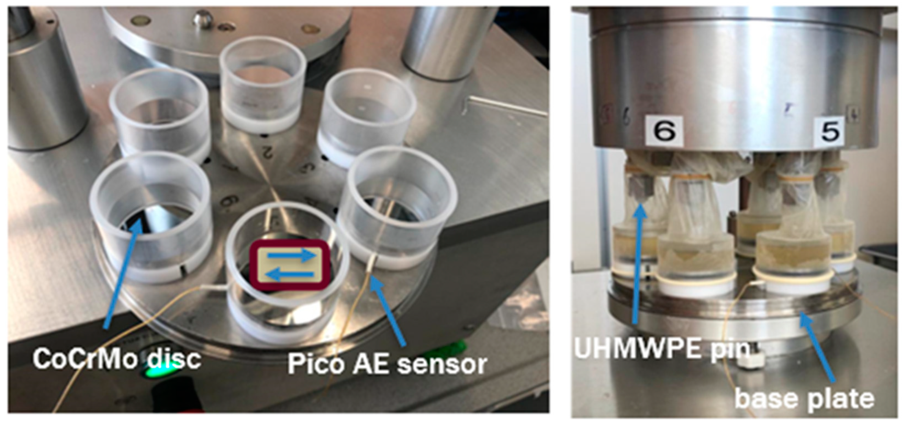
2.1. Tribotests

Multi-directional pin-on-disc tribotests [2] were performed using UHMWPE pins sliding against CoCrMo discs in lubricated conditions on a six-station multi-directional tribometer OrthoPOD^® (AMTI, Watertown, MA, USA, Figure 1). OrthoPOD is a multi-directional pin-on-disc tribometer replicating complex human joint motions necessary for accurately simulating the wear of PE joint implants. This tribometer is primarily used to measure the wear of the implants and does not measure the friction coefficient reliably. This tribometer is based on cross-shear motions between implant components used for prostheses. This simulator was particularly used to simulate a rectangular path with lengths A = 2 mm and B = 15 mm, resulting in a cross-shear ratio of 0.12. This represents the typical physiological movement conditions in a human knee for level-walking, and an increase or decrease in the cross-shear ratio might lead to knee failures [1,12,31]

CoCrMo discs were ground and polished to a mirror-like surface with a roughness of Ra < 5 nm. UHMWPE pins were machined from stock Sulene^®-PE (Zimmer Biomet, Winterthur, Switzerland) to be representative of the state obtained on PE lines for hips or knee joints. Initial pin observations using an optical microscope showed that they are not mirror polished and show scratches in the machining direction. UHMWPE pins were gamma sterilized with an irradiation dose of 25–40 kGy under a nitrogen atmosphere [2]. The pins were pre-soaked in the test liquid for one week before the test.

A detailed description of the complete wear setup can be found in a recent study by Dreyer et al. [2]. A normal load of 110 N was applied to the UHMWPE pins, whereas three pins had a diameter of 3.1 mm, and the other three had a diameter higher than 3.1 mm. Therefore, the contact pressure in the flat-on-flat contact was 14.6 MPa for the Ø 3.1 mm pins. The tribotests were performed simultaneously on the six stations of the OrthoPOD. The tests were run for slightly more than four weeks at a frequency of 1 Hz, with interruptions after each week for weighing and replacement of the test liquid. Each test was run for a total of 2.28 million cycles. The test was performed at 37 ± 1 °C in bovine calf serum (BCS, Hyclone™ Calf Serum Lot#AF29165348, GE Healthcare Lifesciences, Chicago, IL, USA), which was diluted with deionized water to a protein concentration of 20 g/L, a commonly used test liquid for knee joints according to ISO 14243-1 [42]. In addition, 7.44 g/L ethylenediaminetetraacetic acid disodium salt dihydrate (Sigma Aldrich, St. Louis, MO, USA) and 2.4 g/L sodium azide (Sigma Aldrich, St. Louis, USA) were added according to the ASTM F732-17 [2] standard to reduce precipitation of calcium phosphate and prevent bacterial growth, respectively. Eventually, a 0.7 µm filter was used to filter BCS with the added substances.

The test liquid was replaced weekly. To limit the evaporation of water from the test liquid, to inhibit dirt from entering the contact, and to avoid air entering the contact, a latex condom is used to seal the contact after the test fluid is added. The test conditions are summarized in

Table 1. Test conditions for multi-directional tribotest on Orthopod.

Parameters	Values
Materials	UHMWPE (pin diameter 3.1 mm), CoCrMo disc
Temperature	37 °C
Rectangular path length	A = 2 mm B = 15 mm Cross Shear = 0.12
Cycles	2,280,000
Load	110 N
Contact pressure	14.6 MPa

.

2.2. Data Acquisition

The CoCrMo discs were designed in such a way that they could hold an AE sensor at the bottom. A Poly-Oxy-Methylene (POM) spacer connected the discs to the test machine bed. Acoustic Emission data were recorded with a standard Vallen AMYS-6 multi-channel data acquisition system. This high-performance AE data acquisition system has been shown to be extremely effective for AE signal processing [20]. A PICO AE micro-miniature sensor with a wide frequency range of 200–750 kHz from Physical Acoustics Corporation (PAC), was used at the bottom of the CoCrMo disc to acquire the AE signals. The sensor’s small size makes it an ideal candidate for applications requiring wideband AE response and sensitive measurements.

As shown in Figure 1, two of the six CoCrMo discs (in articulation with Ø 3.1 mm pins) were fixed with the PICO AE sensor at the bottom to obtain AE signals. Both tests showed similar AE data after processing. Therefore, Acoustic Emission data from a single test was used for feature extraction and in Machine Learning algorithms for classification. A small-diameter, integral co-axial cable exits the sensor side with a BNC connector on the other end. This sensor ensured a wide range of frequencies over which wear mechanisms are known to occur [20,37]. The disc holders were made of Poly-Oxy-Methylene (POM) material, which ensures good AE signal transmission. Since the sensor was attached to the bottom of the sliding metallic contact surface using superglue, it also ensured good transmission of the signals to the Vallen data acquisition system. The other BNC end of the sensor was attached to a pre-amplifier. The sampling rate during AE data acquisition was 2 MHz to fulfill Nyquist’s theorem [43]. An amplifier with an integrated bandpass filter between 95–1000 kHz (2/4 pre-amplifier) was used to amplify the AE signals generated during the test. A large dataset implies a better quality of wear classification of the surface states. A 40 dB gain was used in the amplifier as the signals in this contact have very low amplitudes. Recorded AE signals were obtained in continuous waveforms.

2.3. Wear Measurement

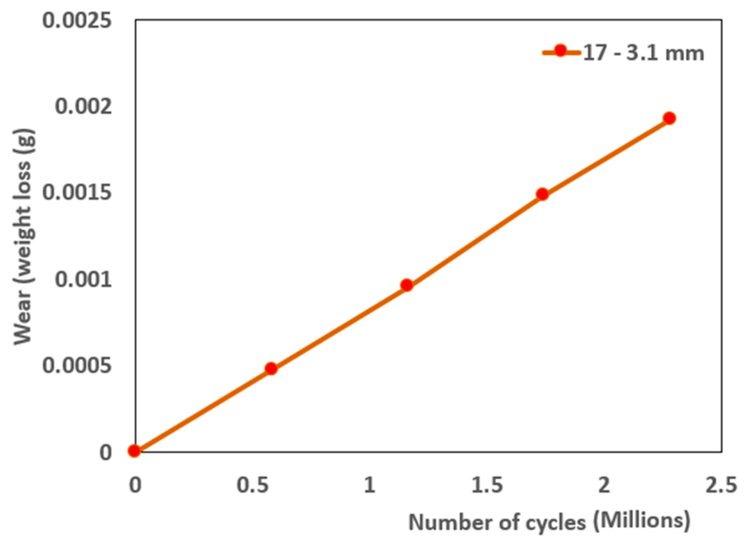
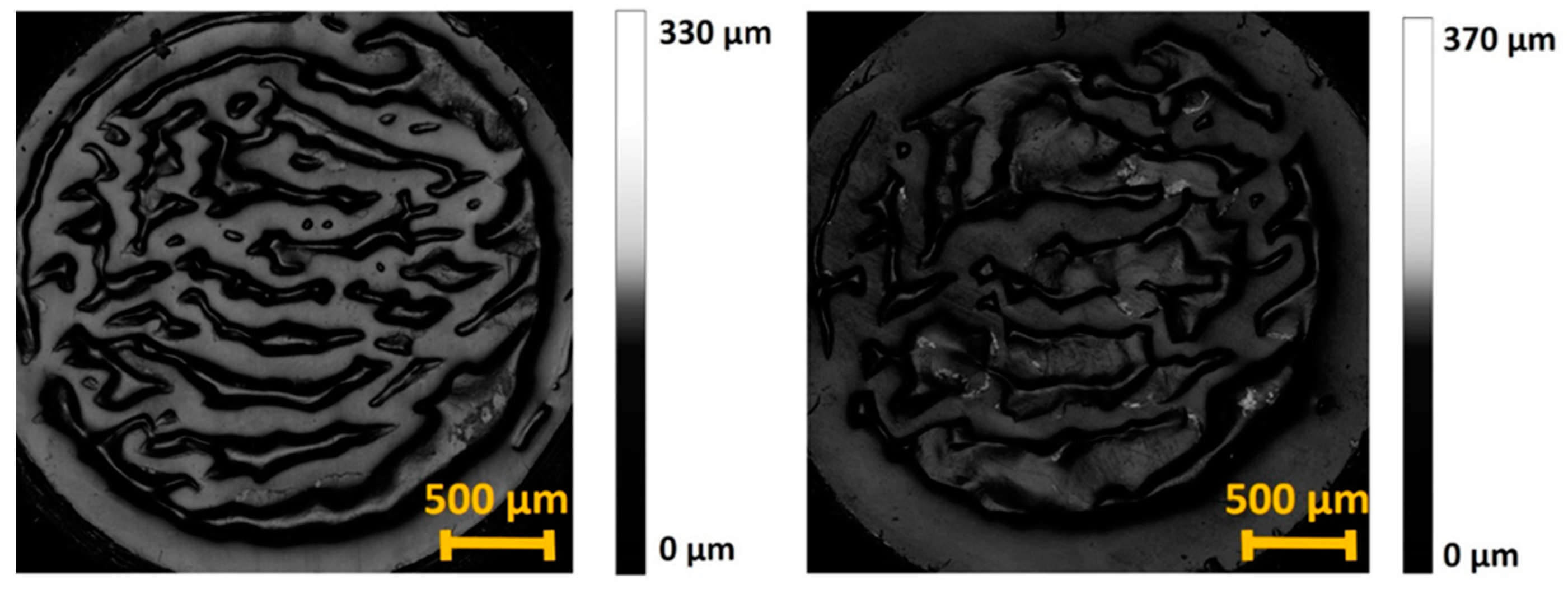
After each test period, both the disc and pin samples were thoroughly cleaned using ultrasonication with acetone and isopropanol as solvents. Then, according to ASTM standard F732-17 [2], gravimetric analysis was performed on the pins using a Mettler Toledo precision balance. These wear measurements were performed on all six tested pins, and the wear rates were similar, with no significant differences. The surfaces of all the CoCrMo discs were observed to verify if third-body wear had occurred, scratching the surface of the discs. However, the wear track was not clearly visible, and the third-body wear was minimal on the metallic counter body. Moreover, the surface evolution of the UHMWPE pins was observed using a Leica optical microscope. The weight losses and the structural features of the optical images on all the UHMWPE pins were found to be similar. In addition, wear volume was measured only on UHMWPE pin no. 17 using an S Neox Sensofar optical profilometer. These were quantitative wear measurements on the protrusions observed on UHMWPE pins compared to qualitative wear measurements in the case of the optical microscope. Due to a lot of variation in the depths of protrusions, a focal variation technique was used to measure the volumes of the protrusions.

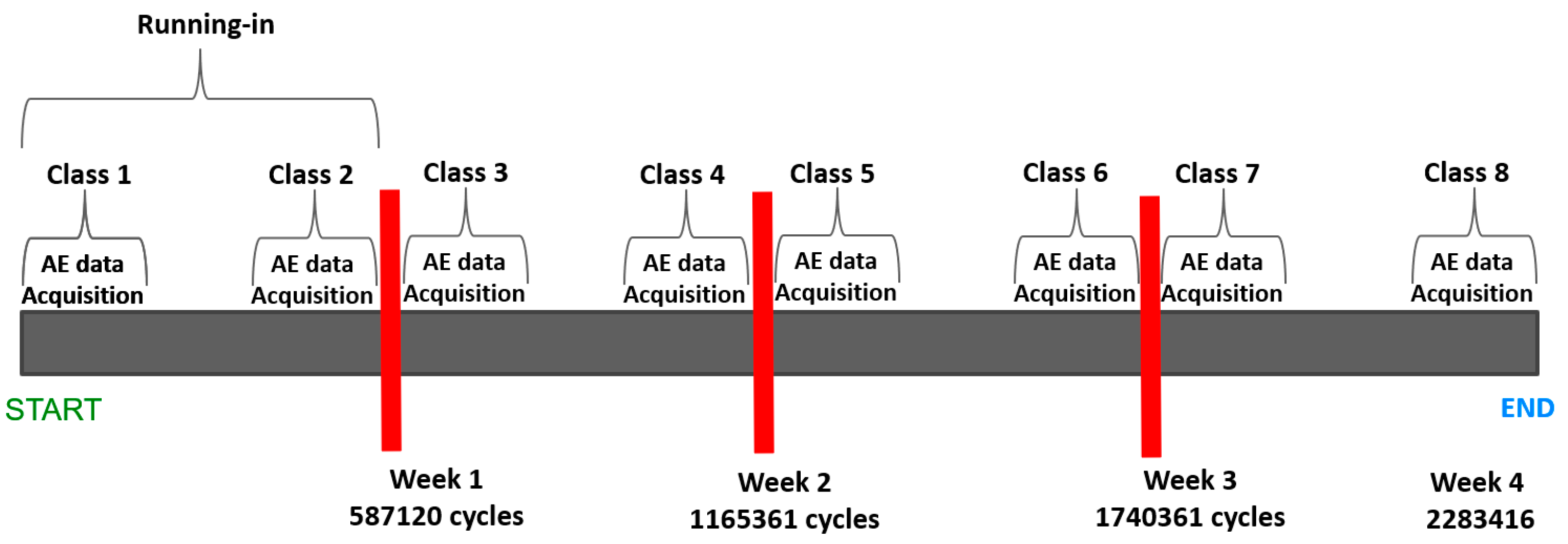
2.4. Wear Classification

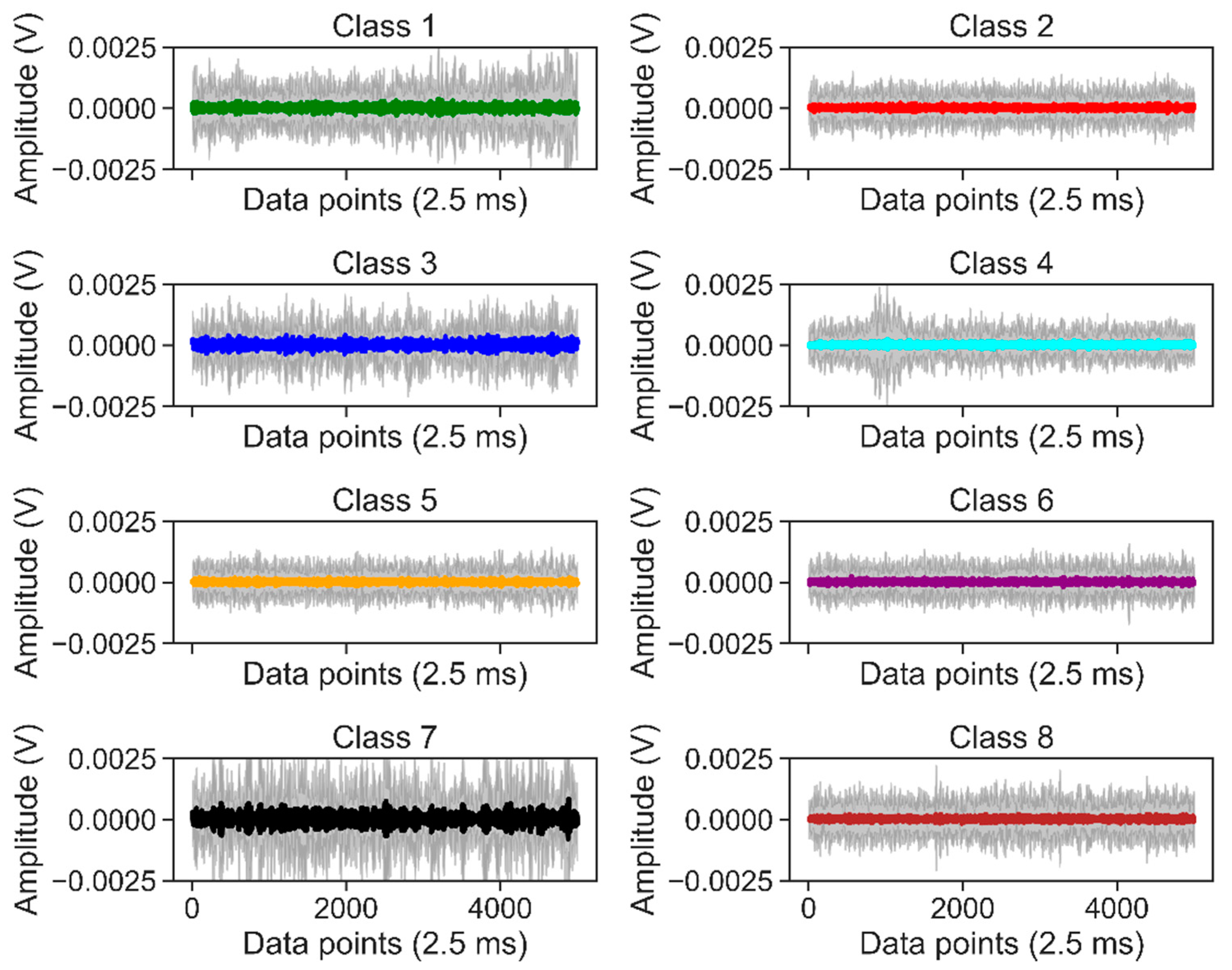
The stages of the AE data acquisition are defined into different wear classes as the surface states change over the course of the test. AE signals were collected in different test stages, as shown in Figure 2. The effective contact surface changed when the rough pin surface was smoothened by wear at the beginning of the test. Samples were re-mounted on the OrthoPOD^® tribometer. A change in the surface states was expected during the entire test duration [7,30].

The red bars indicate the test interruptions. The first AE data acquisition at the test’s beginning is classified as Class 1. Class 1 involves the initial running-in period. Before stopping the test for the first time after close to half a million cycles, AE data are acquired for at least 5 min, and that is defined as Class 2. Class 1 and Class 2 involve a lot of asperity-asperity contact between the UHMWPE pin and CoCrMo disc. Class 3 is where the AE data are acquired just after stopping the test after week 1. Class 4 to Class 8 are defined similarly, as shown in Figure 2. After each stoppage, the disc and the pin samples are thoroughly cleaned with solvents and put back in the pin and disc holders for further testing.

2.5. Data Processing Pipeline

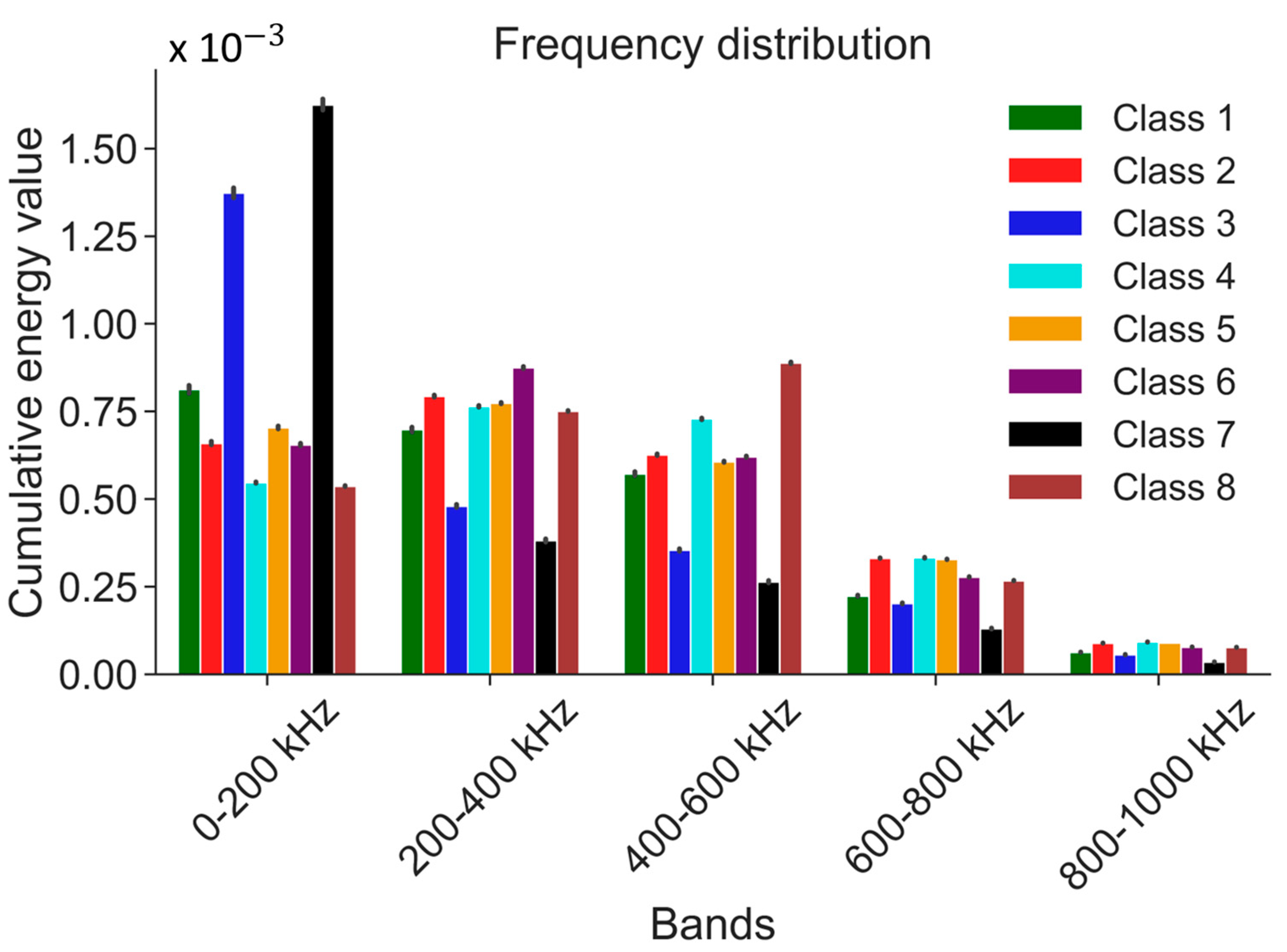
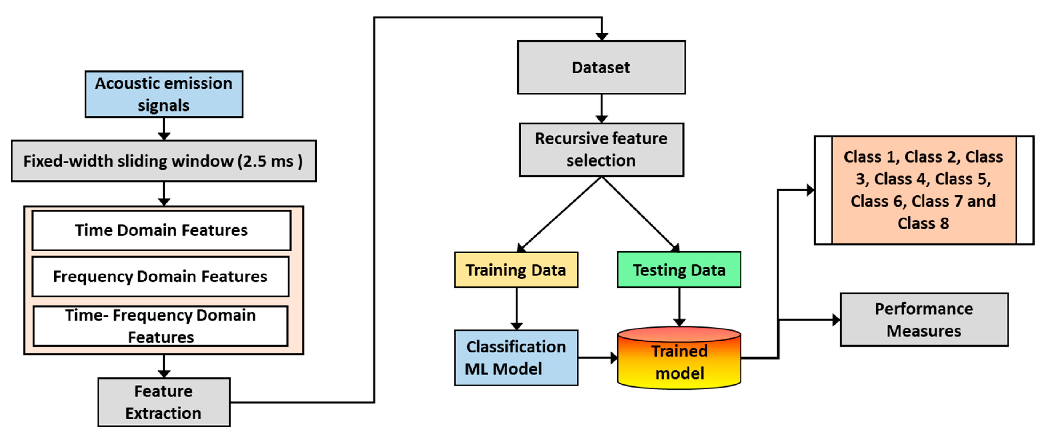
In this specific scenario, we focused on processing raw AE sensor data to extract meaningful features and perform classification based on wear volume measurements and gravimetric analysis. We initiated the process by segmenting the raw data into fixed sliding windows with a duration of 2.5 milliseconds, resulting in 5000 data points per window due to a sampling rate of 2 MHz. We then categorized these sliding windows into eight different classes based on the time at which AE signals were recorded during the test acquisition time. Finally, we proposed two frameworks for feature extraction and classification.

The first framework involved performing manual computations of AE features. Manually extracted vectors representing time, time-frequency, and frequency domain features from each sliding window were used. We applied normalization to ensure fair comparisons among the features, which standardized their scales and prevented any single feature from dominating the subsequent analysis. Following feature extraction and normalization, we employed a recursive feature elimination technique using Logistic Regression (LR). This iterative process involved evaluating each feature’s significance and predictive power using LR. We progressively eliminated less informative or less significant features, resulting in a refined feature set. After the recursive feature elimination, we obtained the top 32 features that were considered the most relevant for the classification task. In the second framework of this specific scenario, we introduced a contrastive deep learning network for feature extraction and classification of the AE sensor data. This approach aimed to automatically learn meaningful AE signal representations automatically without manual feature engineering. We utilized a deep learning network trained using a contrastive loss function. The network learned to map the raw AE signals into a lower-dimensional feature space where similar signals were clustered together and dissimilar signals were separated. This was achieved by encouraging similar AE signals to have nearby representations while pushing dissimilar signals apart. The contrastive loss function compared pairs of AE signals and calculated the similarity between their representations in the learned feature space. During training, the network adjusted its parameters to minimize the contrastive loss, effectively learning representations that captured relevant patterns and characteristics of the AE data. Once the deep learning network was trained, the learned representations were used as features for the classification task. These representations encoded the most informative aspects of the AE signals, enabling more accurate and efficient classification. By leveraging the power of deep learning and contrastive learning techniques, this framework aimed to automate the feature extraction process and capture intricate patterns in the raw AE sensor data. This approach eliminates the need for manual feature engineering. It allowed the model to learn directly from the data, potentially leading to improved performance and better predicting wear classes based on the AE sensor data.

These features, computed by two methodologies, served as inputs for classification algorithms. Following this pipeline, which included sliding window segmentation and feature extraction, our goal was to accurately predict wear classes based on the AE sensor data. We allocated 75% of the subset feature dataset for training the model and used the remaining 25% for testing. We validated this ML approach by using several ML algorithms such as LR, Support Vector Machines (SVMs), Neural Networks (NNs), Naïve Bayes (NB), k-Nearest Neighbor (k-NN), eXtreme Gradient Boosting (XGBoost), and Random Forest (RF).

3. Wear Analysis

3.1. Wear Results

Figure 3 shows the plot of accumulated average weight loss (using gravimetric analysis) vs. the number of cycles in millions on the UHMWPE pin no.17 with a 3.1 mm diameter. Average weight loss was constant (0.005 g) for each test interval, suggesting a linear loss in pin weight against the number of cycles (sliding distance). The wear observed on the other two pins was similar and measured to be around 5 mg/million cycles. Based on these results, it can be concluded that the wear rates remain constant with the number of cycles. It is challenging to confirm two-stage wear (running-in and steady state) from the above plot of average weight loss vs. number of cycles. However, due to the differences in roughness between the pin and the disc, during the run-in, the pin surface was smoothed. The resulting wear rate remains almost constant.

Optical images of the pin were captured after each test period, as shown in Figure 4. Four images are shown: Class 2, Class 4, Class 6, and Class 8. The evolution of the pin surface could be observed in the images. However, optical microscopy provides qualitative information but no information on the size and depth of the protrusions.

Therefore, we measured wear volume using the S Neox optical profilometer. Figure 5 clearly shows distinct images of the wear progression on the UHMWPE pin 1 after Class 4 and Class 6, for example. The evolution of wear is clearly observed. The smaller protrusions are observed to grow larger as we move from Class 4 to Class 6. The optical profilometer’s measured wear volume is 0.977 mm³ after Class 4 and 1.42 mm³ after Class 6, which is in excellent agreement with the gravimetric wear measurements. The protrusions are found to have higher hardness and crystallinity, as shown in the previous research work on the characterization of the UHMWPE pins [2,5]. The pin is worn down progressively, increasing the size of the protrusions further. The increase in the size of protrusions with the progression of the test suggests that the material is constantly removed from the pin, and therefore abrasive wear of UHMWPE pins is the dominant wear mechanism in this contact.

Moreover, UHMWPE particles are continuously produced due to abrasive wear during the test. Protrusions are progressively formed and evolve as the number of cycles increases. Certain protrusions are formed after Class 4. These are more pronounced in terms of depth and morphology after Class 6. The increase in the size of protrusions could be attributed to an increase in abrasive wear between the UHMWPE pins and the CoCrMo discs. However, the weight loss of the UHMWPE pin over half a million cycles was found to be similar. This shows that the wear rate is constant during each period before the test stoppage. The similar loss of material from UHMWPE pins modifies the surfaces of the pins progressively, as observed with the change in morphology and depth of protrusions. This gradual wear producing UHMWPE debris particles can lead to implant failure through implant loosening [5,6,7,36]. Therefore, observing whether the gradual and progressive weight loss and sample surface changes affect the AE signals and could be separable via ML will be interesting.

3.2. Exploratory Data Analysis

Figure 6 illustrates the raw AE signals for eight defined wear classes. Examination of the raw AE signals shows that the signal’s amplitude is the highest in Class 7. Class 1 shows higher amplitude than other classes but less than Class 7. The amplitude then decreases in Class 2, and the amplitude for Class 3 is intermediate between Class 1 and Class 2. Class 1 shows the highest amplitude due to the wear during the initial running-in period. However, Class 4 and Class 5 exhibit a decrease in signal amplitude, while Class 7 shows another increase. Class 4 still shows some single spikes at the beginning of the acquisition, and then the signals stabilize. Class 8 showed more signal spikes of higher amplitude than Class 6, which could be attributed to the progressive abrasive as well as third-body abrasive wear occurring due to the UHMWPE debris particles increasing over time after Class 7. Class 1, Class 3, and Class 7 show high-amplitude signal spikes due to the restart of the test after the samples were cleaned. Overall, no apparent, discernible trends are evident from the raw AE signals alone.

Signal processing analysis techniques and statistical feature visualization are necessary to analyze the data further and extract meaningful information. The plots of raw AE signals in Figure 6 utilize a rolling window across the time series. However, these plots do not reveal any distinctive patterns or valuable insights when examined solely across the time series data for the eight classes. Hence, a comprehensive analysis is essential to understand the underlying patterns and identify unique characteristics among the different classes. Signal processing plays a crucial role in the analysis of intricate AE signals. Initially, the signals are filtered using a bandpass filter, so there is no anti-aliasing. A low-pass filter of 1 MHz was applied. Next, features are extracted from the filtered AE data, considering time, frequency, and time-frequency domains. Visualizing the distributions of these features across different categories offers valuable insights into their discriminatory power, informativeness, and ability to detect outliers. Such visualizations assist in understanding decision boundaries and inspire effective feature engineering, enhancing the accuracy and performance of ML classification models.

3.3. Time Domain Feature Analysis

In the time domain, signals are typically represented as a function of time, with time as the independent variable and the signal’s amplitude or value as the dependent variable at each time point. This representation allows for the analysis and visualization of signal changes over time. Time domain features encompass measures like harmonic mean, skewness, RMS distributions, kurtosis, crest factor, standard deviation, minimum, maximum, median, and more [20]. In this particular case, Figure 7 and Figure 8 focus on the harmonic mean and RMS distribution across the eight distinct wear classes. The violin plots in Figure 7 reveal noticeable differences in characteristics, such as variations in shape and size, among the different wear classes. This enables seamless utilization of the top 32 extracted features as inputs for ML algorithms in classification and prediction tasks. In addition, this visual representation quickly discerns significant disparities in feature values between classes.

Figure 8 explicitly illustrates the RMS distribution for all eight classes, demonstrating their distinguishability. The density of the RMS distribution varies across different classes, and the distribution of RMS features also changes from one class to another. Additional time domain features, such as variance and standard deviation, were also analyzed, but their statistical characteristics showed less distinct patterns. Therefore, optimizing the time domain features based on their sensitivity is necessary to distinguish the eight categories. These optimized features can then be used as inputs for ML algorithms.

3.4. Frequency Domain Analysis

The transition from the time domain to the frequency domain revealed distinct patterns in the AE signals that repeat over specific time intervals. These periodic patterns were identified by applying the Fourier Transform, which allowed for the determination of the frequency range associated with these events across the eight wear classes. To quantify the frequency content of the signals, the Power Spectral Density (PSD) was calculated using the periodogram method with a window size of 2.5 ms [44]. The PSD provides information about the distribution of signal power across different frequencies. Analyzing the PSD, we could observe the relative strength of different frequency components within each wear class. Figure 9 illustrates the PSD distribution for the eight wear classes. The distribution of Power Spectral Density exhibits distinctive characteristics across all eight wear classes within five different frequency windows: 0–200 kHz, 200–400 kHz, 400 kHz–600 kHz, 600–800 kHz, and 800 kHz–1 MHz. These frequency windows were selected based on the sampling rate of 2 MHz. The periodogram analysis revealed statistical separation among the wear classes. This implies that the PSD features can effectively discriminate between different wear classes.

Consequently, the Power Spectral Density and periodogram features can be used as inputs for ML classification algorithms, enabling real-time wear classification. Analyzing the magnitude of the bar plot representing the PSD provides insights into how the feature values vary within each wear class across different frequency windows. If the distributions of these features exhibit significant differences among the wear classes, it indicates that these features can serve as effective discriminative factors for classification purposes. Overall, the frequency domain analysis, including calculating Power Spectral Density and utilizing periodogram features, provides valuable insights into the frequency content of AE signals and enables the identification of distinctive characteristics that aid in wear classification.

4. Machine Learning Classifier

Feature extraction is vital in preparing AE time series data for ML classifiers. Its main objective is to extract specific attributes or characteristics that can provide meaningful information for classification, prediction, and other analytical tasks. In the context of AE time series data, the raw sensor data are divided into fixed-width sliding windows with a duration of 2.5 ms, facilitating subsequent analysis. Each sliding window yields a vector comprising multiple statistical features that capture valuable information across diverse domains, encompassing time, frequency, and time-frequency. These features serve as a means to gain insights into the underlying patterns and variations inherent within the AE signals. By harnessing these statistical features from distinct domains, ML classifiers are equipped to effectively analyze AE time series data, enabling tasks such as anomaly detection, fault diagnosis, and structural health monitoring. These extracted features play a pivotal role in aiding the classifiers in recognizing patterns, making precise predictions, and executing dependable classifications based on the rich information acquired. For specific details regarding the features and their calculations, kindly refer to

Table 2. Time, frequency, and time-frequency domain features were extracted from each raw sliding window.

Domain	Feature
Time	Mean, RMS, Kurtosis, Skewness, Crest factor, Standard deviation, Minimum, Maximum, Median etc.
Frequency	Position of peaks with high intensity, Energy distribution in respective energy bands
Time-frequency (Wavelet)	Enthalpy, RMS, Kurtosis, Skewness, Standard deviation in respective decomposition levels etc.

, which furnishes a comprehensive compilation of time, frequency, and time-frequency domain features extracted from each raw sliding window.

The ML classifier pipeline consists of several crucial steps for preprocessing and analyzing data, as shown in Figure 10. It begins with sliding window segmentation, dividing the raw data into fixed-width sliding windows to capture temporal information and create smaller segments for analysis. Each window extracts a vector of features, including statistical measures, spectral characteristics, or time-frequency domain representations. In this work, 294 features were initially used. After feature extraction, recursive feature elimination is applied to select the most relevant features based on classifier performance or predefined criteria. This iterative process results in an optimal subset of features.

In this case, LR-based feature selection was used to pick 32 informative features to train the classifier, ensuring accuracy without compromising the feature subset. The next step involves preparing a new feature subset containing the selected 50 features for the classification task. Stochastic selection allocates 75% of the data for training and 25% for testing the models. Finally, the ML classifiers are trained and evaluated using the new feature subset, learning patterns, and relationships within the data to make accurate predictions or classifications. Performance evaluation is conducted using metrics such as classification accuracy. As illustrated in Figure 10, this comprehensive data treatment pipeline ensures that relevant information is captured, irrelevant features are eliminated, and the classifier is trained on a focused and informative feature set, improving classification performance.

Classification Results

This study employed a combination of two linear and four non-linear ML classifiers: LR, SVM, k-NN, RF, NN, and XGBoost. The training parameters for the chosen classifiers were determined using empirical guidelines as outlined in

Table 3. Training parameters of the classifiers for predicting classes.

Classifier Type	Parameters	Values
Support Vector Machine (SVM)	Validation method	RepeatedStratifiedKFold
	SVM kernel function	Radial basis function
	Gamma scale	Automatic
	Features	50 Subset features
	Multi-class method	One-vs.-rest
	Standardize data	True
k-Nearest Neighbor (k-NN)	Classifier	Minkowski
	Number of neighbours	15
	Distance metric	Distance
	Distance weight	Uniform
	Validation method	RepeatedStratifiedKFold
Neural Networks (NN)	Number of neurons	60, 40, 20
	hidden layer	3
	Training method	Backpropagation
	Performance	Cross-entropy
	Epoch	5000 iterations
	Validation method	RepeatedStratifiedKFold
XG Boost	Rate of learning	0.3
	Tree_method	Auto
	Depth	6
	Sampling method	Uniform
	gamma	0.1
	Validation method	RepeatedStratifiedKFold
Random Forest (RF)	Validation method	RepeatedStratifiedKFold
	n_estimators	100
	Split criterion	Gini’s diversity
	max_features	sqrt
Logistic regression (LR)	max_iterations	1000
	penalty	L2
	Validation method	RepeatedStratifiedKFold

. Their performance was assessed by considering prediction accuracy. In future endeavors, the training parameters of these classifiers can be further refined, considering factors such as training time and prediction accuracy, which will be addressed in our upcoming research.

Table 4. Accuracies for predicted label (wear classes) vs. true label (ground truth) on eight classes.

Groundtruth Accuracy [%]	Class 1	Class 2	Class 3	Class 4	Class 5	Class 6	Class 7	Class 8
Class 1	93	2	0	2	2	1	0	0
	83	3	1	6	5	1	1	0
	91	1	0	4	3	1	0	0
	93	1	0	3	2	1	0	0
	88	2	1	6	3	0	0	0
	85	1	1	7	3	2	1	0
Class 2	1	70	5	14	5	5	0	0
	2	58	5	19	9	7	0	0
	1	67	5	16	7	4	0	0
	0	74	4	13	4	5	0	0
	1	59	5	19	9	7	0	0
	2	52	6	22	13	5	0	0
Class 3	0	6	82	2	4	6	0	0
	1	6	76	2	9	6	0	0
	1	5	79	2	6	7	0	0
	1	7	82	2	3	5	0	0
	1	5	78	3	8	5	0	0
	1	6	75	3	9	6	0	0
Class 4	1	8	0	84	4	3	0	0
	4	11	0	73	6	6	0	0
	1	7	0	85	4	3	0	0
	1	10	0	81	4	4	0	0
	2	8	0	81	6	3	0	0
	2	7	0	82	7	2	0	0
Class 5	1	4	4	5	86	0	0	0
	2	8	4	6	79	1	0	0
	2	3	3	5	87	0	0	0
	1	5	3	4	86	1	0	0
	2	6	3	8	81	0	0	0
	2	5	3	11	77	2	0	0
Class 6	1	4	2	5	0	88	0	0
	1	5	2	8	1	83	0	0
	1	4	1	7	1	86	0	0
	0	5	1	5	1	88	0	0
	1	5	1	8	1	84	0	0
	1	6	2	1	2	88	0	0
Class 7	0	0	0	0	0	0	99	1
	1	0	0	0	0	0	96	2
	0	0	0	0	0	0	98	2
	0	0	0	0	0	0	99	1
	0	0	0	0	0	0	98	2
	0	0	0	0	0	0	98	2
Class 8	0	0	0	0	0	0	0	100
	0	0	0	0	0	0	0	100
	0	0	0	0	0	0	0	100
	0	0	0	0	0	0	0	100
	0	0	0	0	0	0	0	100
	0	0	0	0	0	0	0	100

Tables for the classification accuracy results using the six classifier models (XG Boost, LR, RF, NN, SVM, and k-NN). The classification results in each cell from top to bottom are for: XG Boost, LR, RF, NN, SVM, and k-NN. All values are in %.

provides a comprehensive overview of the classification results, including a confusion matrix and a comparison among six ML algorithms. The accuracies reported in the table represent the percentage of true positives out of the total number of tests for each class. On the other hand, the errors are calculated by dividing the number of true negatives by the total number of tests and are displayed in the non-diagonal cells. To interpret the above confusion matrix in Table 4, XGBoost in the first column is considered an example. The average classification accuracy for the XGBoost algorithm is 87.75%. The extracted features from Class 1 are classified with a high accuracy of 93%. The classification accuracy is high in Class 1 for all the other algorithms, as the surface states are bound to be different in the running-in period. The classification errors are minimal and originate from slight misclassifications into Class 2 (2%), Class 4 (2%), Class 5 (2%), and Class 6 (1%). These misclassifications suggest a slight overlap of features between Class 1 and the other four classes. Similarly, for Class 3, Class 4, Class 5, Class 6, Class 7, and Class 8, the misclassification rates are minimal, indicating that the surface states for these classes are distinct and independent of other wear classes.

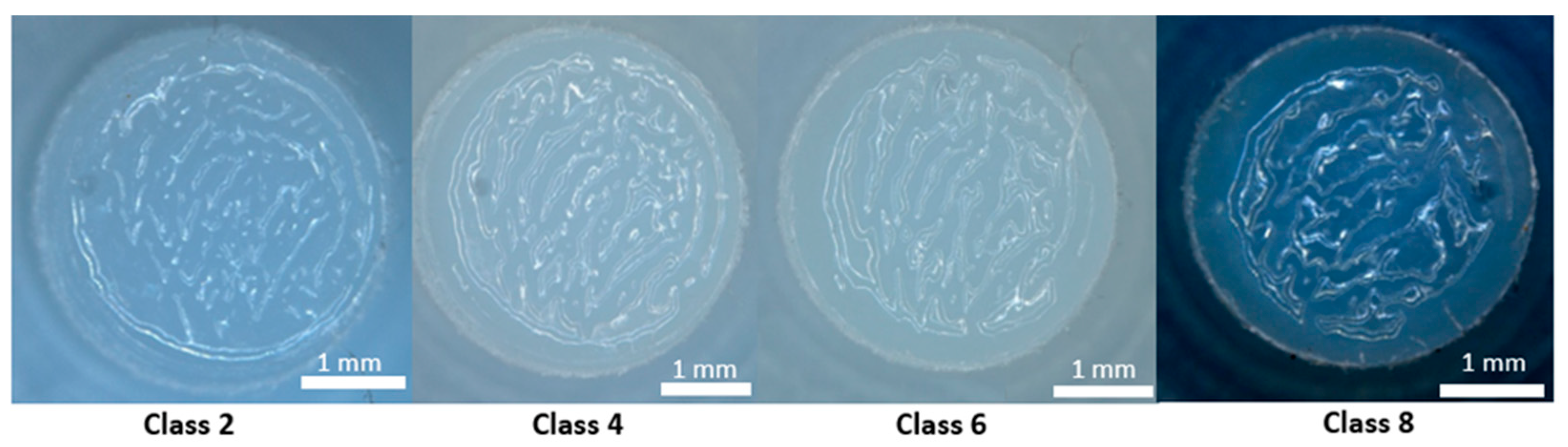
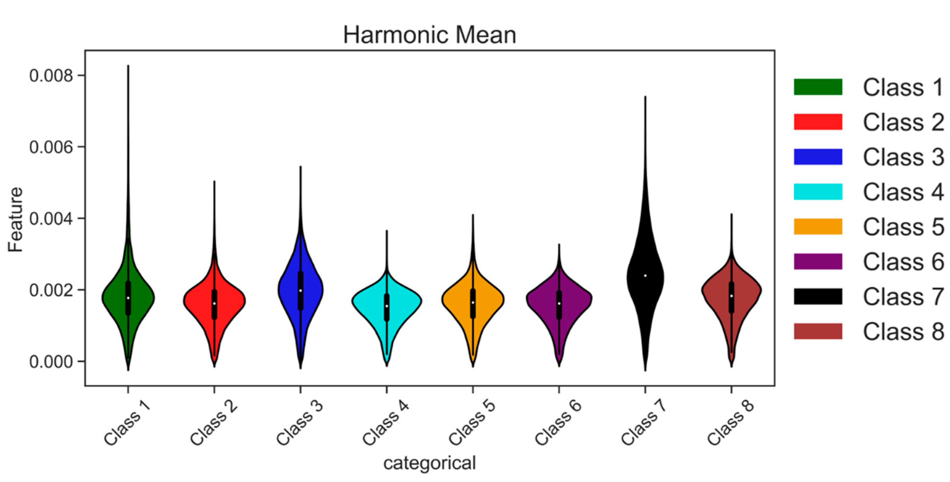
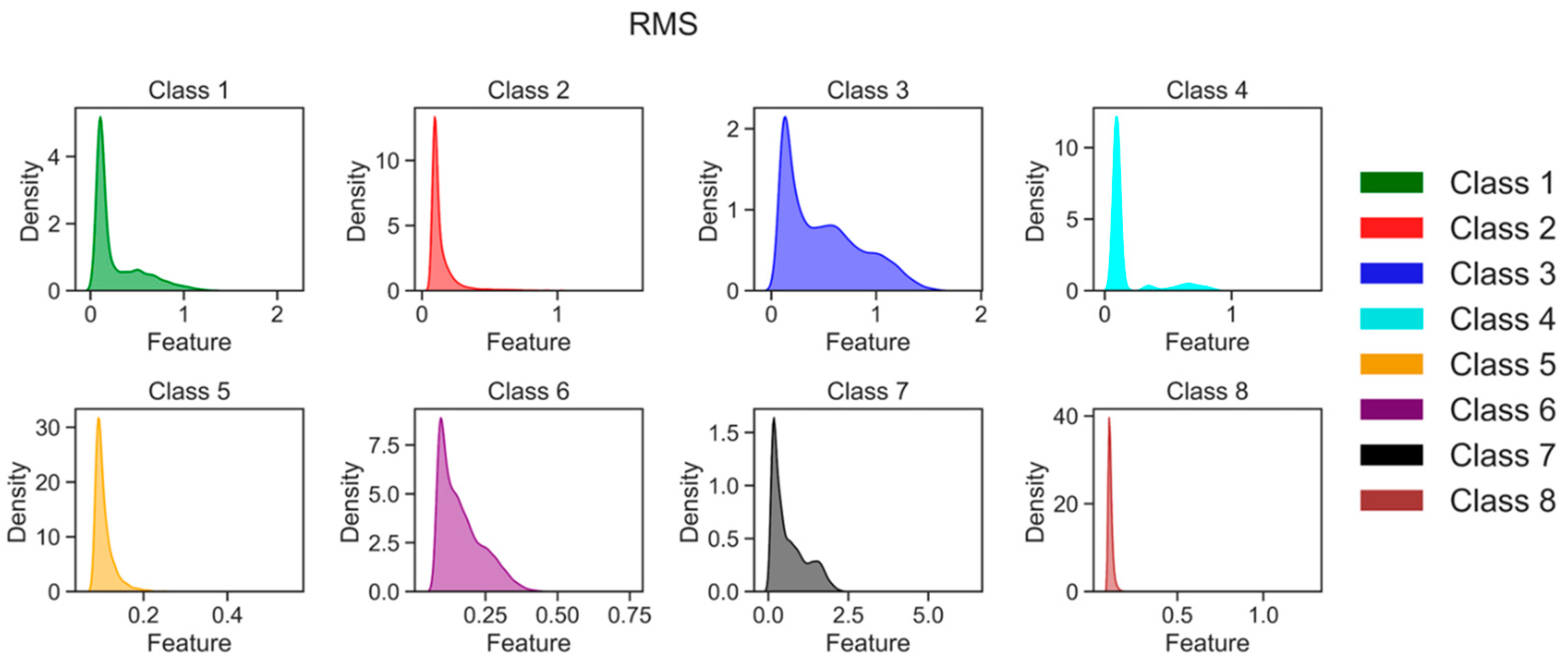
This suggests the progression of abrasive wear in the form of third-body abrasion occurs continuously as we move from Class 3 to Class 8. The UHMWPE debris particles cause third-body abrasive wear. Protrusions are formed through the folding of the UHMWPE, entrapping black debris contamination on the surface of the UHMWPE pins. The size of these protrusions increases with time until the test is completed. Additionally, it is essential to note that the poorest classification results occur at the beginning of the experiment (70% for Class 2) in XGBoost and in the case of all the other ML algorithms. This may be attributed to the running-in period, where changes in surface roughness are the most significant. However, after the running-in period (Class 3 onwards), the classification accuracy improved significantly, ranging from 82% to 100%. This demonstrates the effectiveness of our approach to classifying wear. Some misclassifications are observed between alternate classes, such as Class 1, Class 3, Class 5, and Class 7, as well as Class 2, Class 4, Class 6, and Class 8. These misclassifications may be attributed to variations in surface conditions, such as fresh and cleaned surfaces with less debris and lubricant contamination for Class 1, Class 3, Class 5, and Class 7, and lubricated and wear debris-filled protrusions constantly increasing in size for Class 2, Class 4, Class 6, and Class 8.

Table 4 illustrates the average classification accuracies obtained on all six ML algorithms, and they are found to be in a similar range and more than 80%. The performance of hand-picked features for classification was unsatisfactory, which may be attributed to the complexity and nuances of the labeled categories. However, these results suggest that our methodology has potential, especially considering the setup was not fully optimized. This combination of AE data processing with ML algorithms holds promise for real-time monitoring of progressive wear in UHMWPE materials used in human joint prostheses.

5. Contrastive Learning

The previous section presented classification results using various ML algorithms on hand-picked features. To overcome the limitations of manual feature extraction, the following section proposes using CNN for automatic feature map extraction. The study will compare the performance of hand-picked features with features computed using CNN. Contrastive learning trains a neural network to distinguish between positive and negative pairs, aiming to create a feature embedding space with closer proximity for similar examples and greater separation for dissimilar ones [45,46,47]. Circle loss offers a different approach to achieving this goal than contrastive loss functions like contrastive loss, triplet loss, or N-pair loss. Circle loss introduces decision boundaries in the form of circles around each instance in the embedding space, intending to promote the inclusion of positive pairs within their respective circles and the exclusion of negative pairs from them [48]. This decision boundary is represented as a circle around each instance, and the objective is to ensure that all positive samples lie inside their respective circles while negative samples lie outside. In summary, using Circle loss within contrastive learning optimizes the learning of feature representations, enabling the network to distinguish between different classes or categories in each dataset effectively.

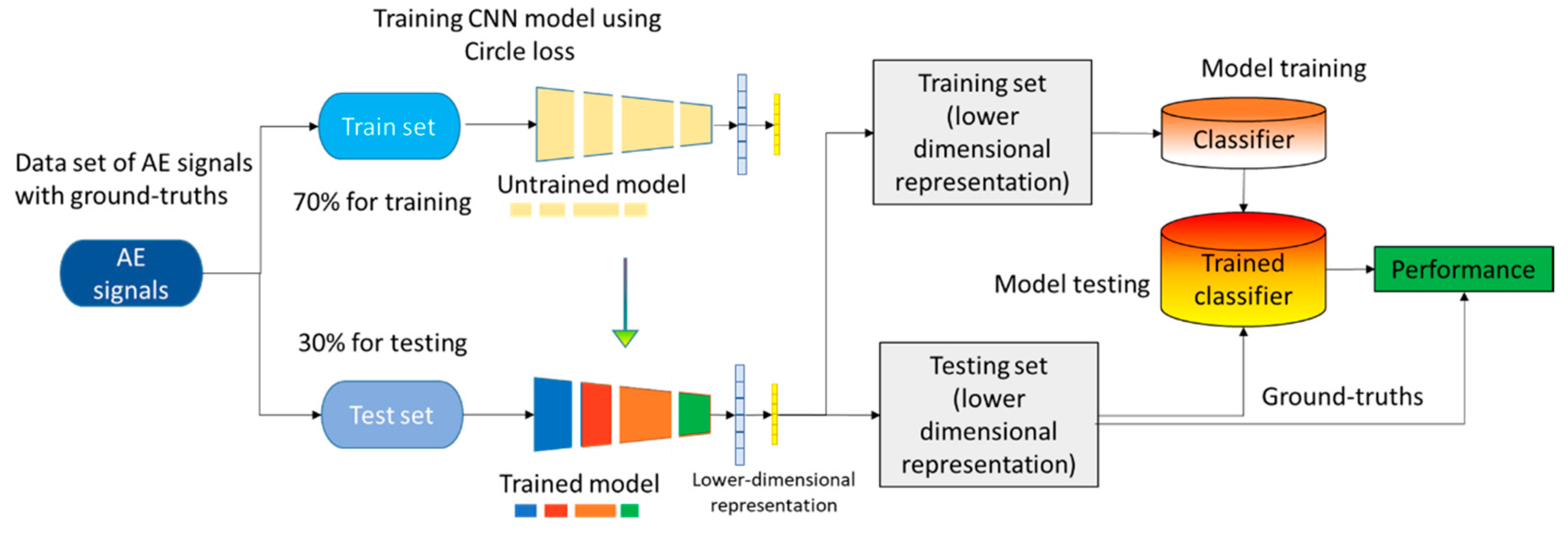
Training a CNN through contrastive learning, specifically employing circle loss, entails three primary steps, as depicted in Figure 11. Firstly, the data preparation phase involves pairing AE signals from distinct categories within the process zone, guided by their degree of similarity or dissimilarity, facilitated by the application of contrastive loss. Pairs that pertain to the same category are marked with a Boolean value of 1, while pairs originating from different categories receive a Boolean value of 0. Subsequently, the subsequent step encompasses constructing a network crafted to capture a lower-dimensional representation of the AE signatures. This network inputs the paired AE signals and generates a feature map as its output. It aims to learn meaningful representations capable of distinguishing various categories based on distinctive AE signatures. Lastly, the network undergoes training employing circle loss, constituting a variation of contrastive loss specifically devised for deep metric learning. This final step ensures that the network’s learned representations effectively facilitate differentiation between the different categories. Circle loss encourages the network to learn discriminative features by forming tight clusters for each category while maximizing inter-class separability. During the training process, monitoring the magnitude of the loss is crucial. The loss should decrease with each epoch, indicating the convergence of the network learning. In the case of multi-class classification in a supervised manner, ML classifiers are trained on the feature map generated by the network. These trained classifiers map the learned features to the corresponding class labels. This approach allows for classifying unseen data based on the learned representations.

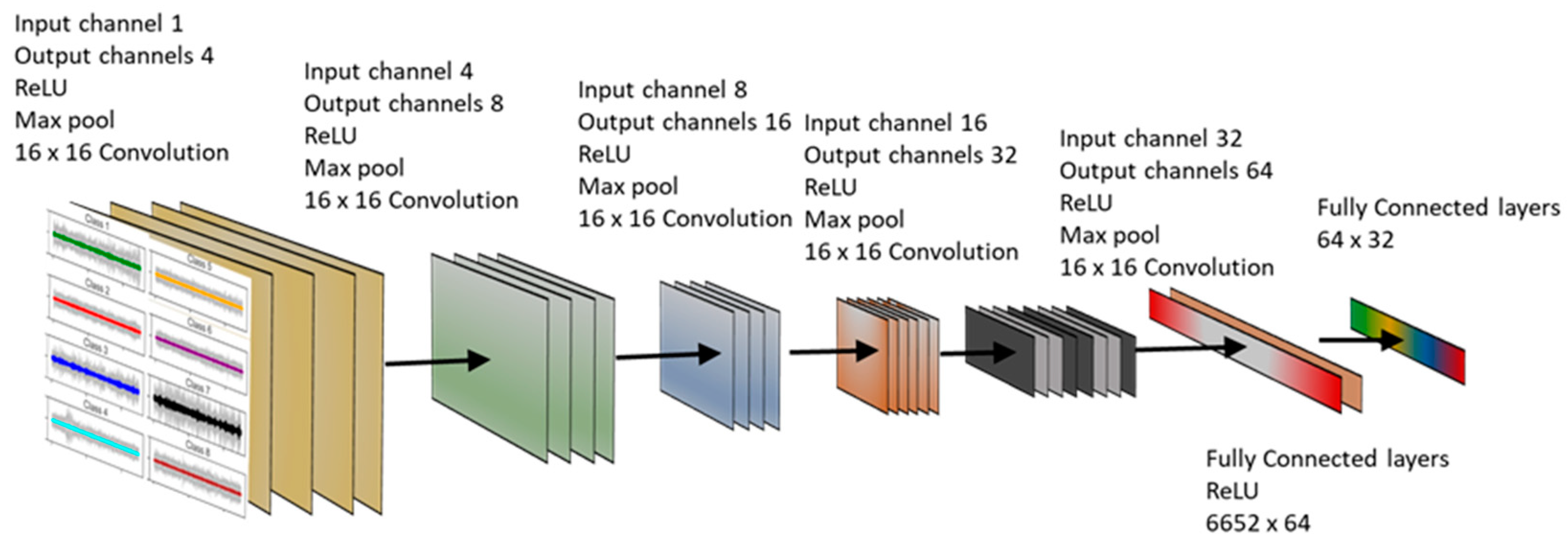
The CNN model was implemented using the PyTorch library (Meta, USA), with a meticulous fine-tuning of 3.5 million parameters to achieve optimal performance. After an extensive search for the optimal design, the final CNN network was developed, consisting of five convolution and three fully connected layers, as depicted in Figure 12. The initial CNN layer takes a tensor of size B (Batch size) × 1 × 5000 as input, representing the length of the AE signal. The network then processes this input to generate a feature map with dimensions B × 32, which is a compressed representation of the original signals. During training, the chosen optimizer was stochastic gradient descent with momentum, facilitating efficient convergence. To extract meaningful features, each convolution layer employed a 16 × 16 kernel. Additionally, a dropout rate of 10% was implemented between each epoch to alleviate the risk of overfitting. The Rectified Linear Unit (ReLU) activation function was applied to introduce non-linearity into the network. A batch size of 256 was used during training to ensure efficient processing. The entire training procedure was conducted on a high-performance Nvidia RTX Titan GPU (Nvidia, USA), enabling accelerated computations and enhancing training performance.

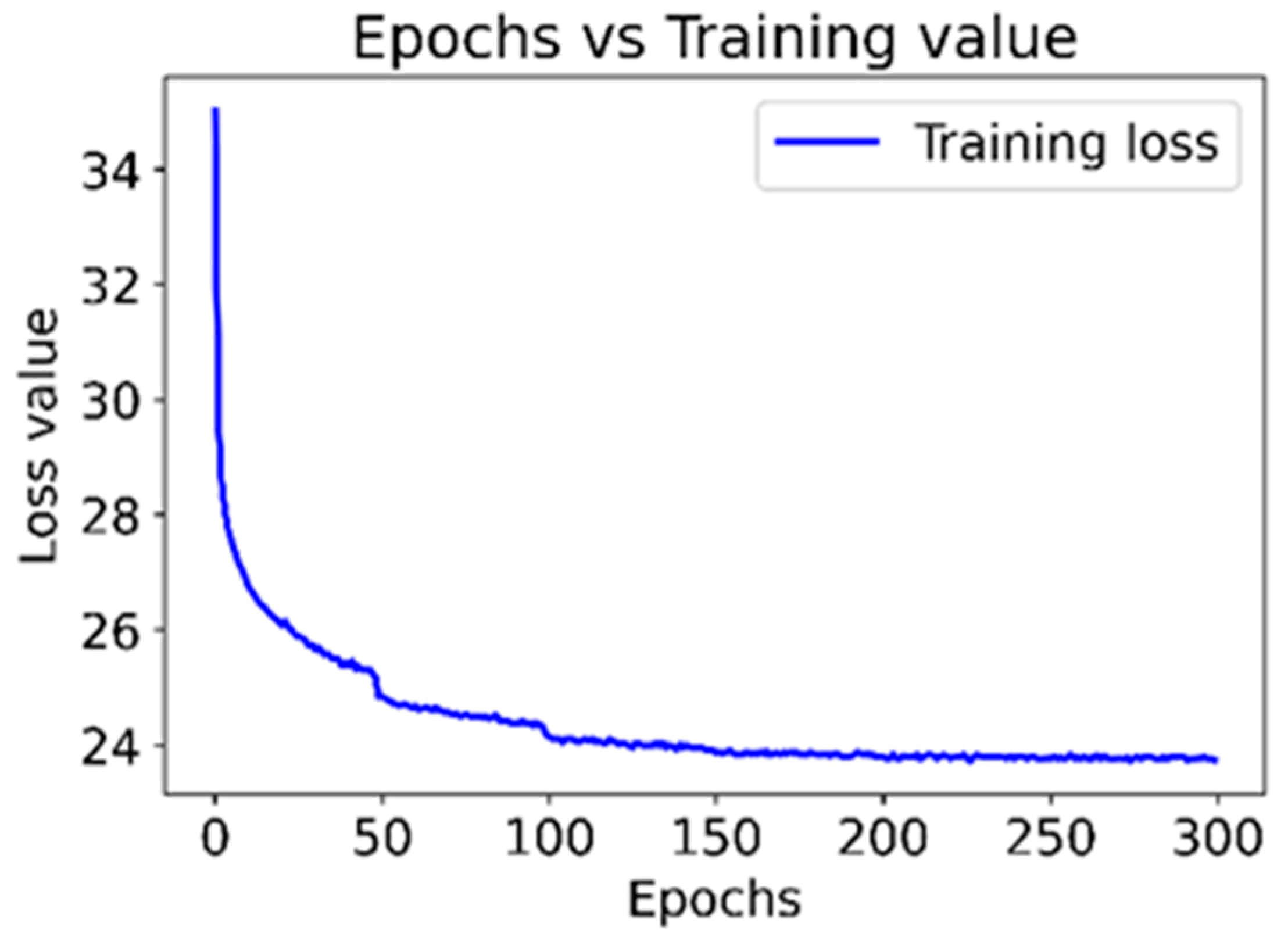
Figure 13 represents the progression of loss values throughout 300 training epochs for the CNN model. The loss values indicate how well the model learns and captures the underlying distributions present in the AE signals. The graph shows a consistent decline in the loss values during the initial 100 epochs, suggesting that the model significantly improves in capturing the desired patterns and features from the input data. Subsequently, no substantial improvement is observed beyond this point, as evidenced by the information depicted in Figure 13. This plateauing of the loss values suggests that the model has likely reached a point of diminishing returns in terms of learning from the training data. Further training beyond this point may not lead to significant enhancements in performance.

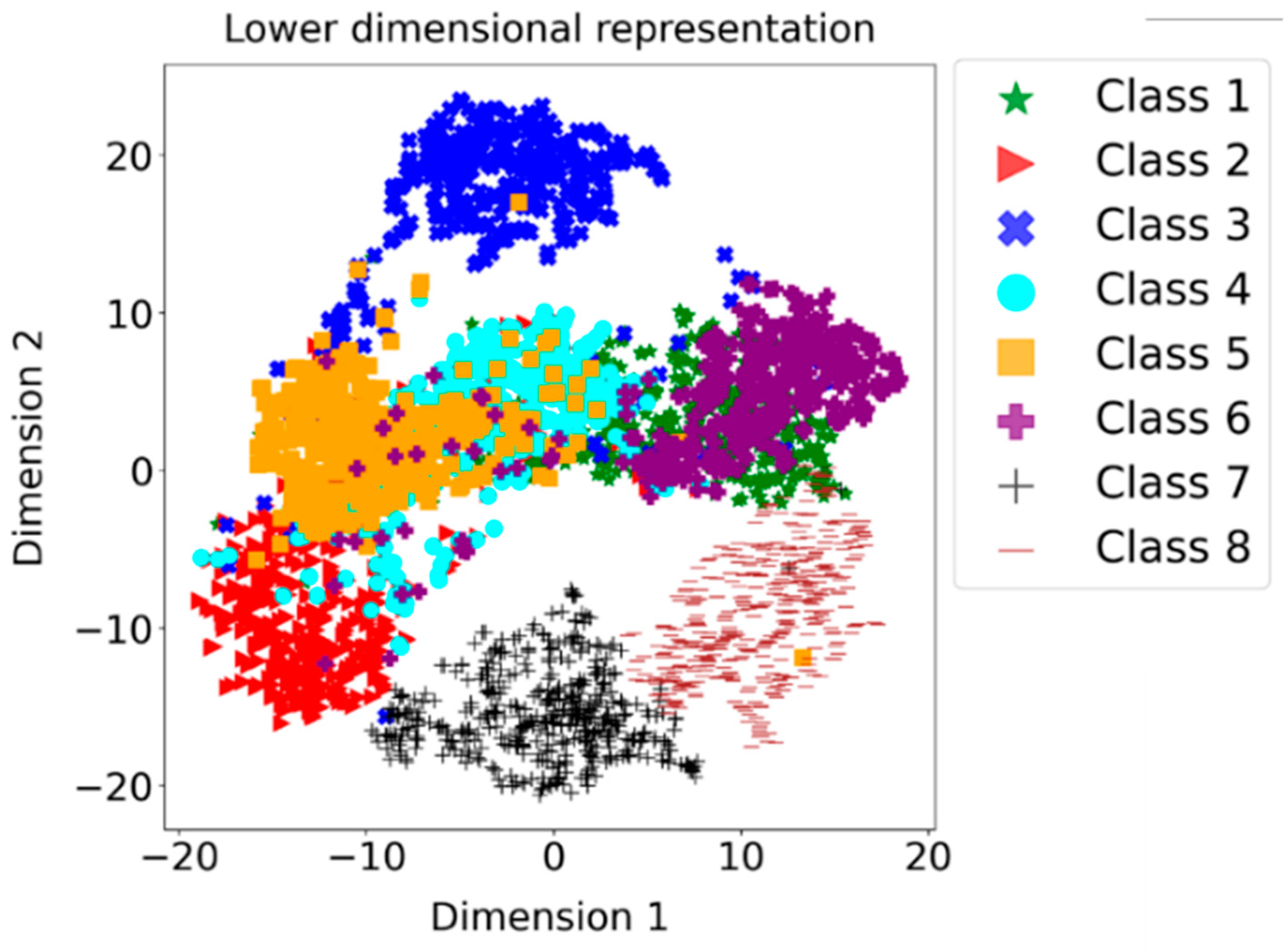
While analyzing loss values is valuable, additional evaluation techniques, such as feature map visualization, can provide a more comprehensive understanding of a model’s performance. One approach to visualizing feature maps is reducing their dimensions and displaying them in a two-dimensional space. Figure 14 showcases the 2D visualization of a reduced-dimensional representation created using t-SNE (t-Distributed Stochastic Neighbor Embedding) on the feature map derived from a CNN trained with contrastive loss. The results presented in Figure 14 reveal distinct clusters for each of the eight classes. This clustering indicates that the CNN, trained using contrastive learning, effectively captures and separates different classes based on their unique features.

This finding highlights the effectiveness of contrastive learning in addressing the monitoring problem. However, it is crucial to acknowledge the presence of certain overlaps in the visualization. These overlaps suggest similarities in the process dynamics that result in overlapping grades. It is essential to carefully analyze and consider these overlaps when interpreting the performance of the CNN model. Overlaps may indicate areas where the model faces challenges in accurately distinguishing between similar classes or where the data contains inherent complexities. By combining loss analysis with feature map visualization, we can better understand the model’s performance, its ability to learn and differentiate classes, and the inherent complexities and overlaps present in the data. This holistic evaluation allows for more informed interpretations and insights into the CNN model’s capabilities. The presence of distinct clusters within the lower-dimensional representation obtained from the CNN trained with circle loss through contrastive learning has motivated us to perform a supervised classification task. In line with the approach detailed in Section 4, we have applied the six ML classifiers. These classifiers adhere to identical training parameters outlined in Table 3, with the lower-dimensional representation employed as input. The classification results are summarized as a confusion matrix, presented in

Table 5. Accuracies for predicted label (wear classes) vs. true label (ground truth) on eight classes.

Groundtruth Accuracy [%]	Class 1	Class 2	Class 3	Class 4	Class 5	Class 6	Class 7	Class 8
Class 1	97	0	1	1	1	0	0	0
	98	0	0	1	1	0	0	0
	95	0	0	3	2	0	0	0
	98	0	1	1	0	0	0	0
	98	0	0	1	1	0	0	0
	96	0	0	2	2	0	0	0
Class 2	1	89	1	8	2	1	0	0
	0	90	0	7	2	1	0	0
	0	87	1	10	2	0	0	0
	0	87	1	9	2	1	0	0
	0	89	1	7	2	1	0	0
	0	91	0	7	2	0	0	0
Class 3	0	1	94	1	2	2	0	0
	0	0	96	1	1	2	0	0
	0	1	93	2	2	2	0	0
	1	1	95	1	1	2	0	0
	0	0	96	1	1	2	0	0
	0	1	91	2	3	3	0	0
Class 4	0	6	0	91	2	1	0	0
	0	5	0	92	2	1	0	0
	0	3	0	94	2	1	0	0
	0	5	2	90	1	1	0	0
	0	4	0	93	2	1	0	0
	0	6	0	90	2	2	0	0
Class 5	0	2	1	3	94	0	0	0
	0	2	0	2	95	1	0	0
	0	1	0	4	94	1	0	0
	0	2	2	3	93	0	0	0
	0	2	1	2	95	0	0	0
	0	2	0	2	96	2	0	0
Class 6	0	1	1	3	0	95	0	0
	0	1	1	2	0	96	0	0
	0	1	1	4	0	94	0	0
	0	1	2	3	0	94	0	0
	1	1	2	0	0	96	0	0
	0	1	0	3	0	95	1	0
Class 7	0	0	0	0	0	0	100	0
	0	0	0	0	0	0	100	0
	0	0	0	0	0	0	100	0
	0	0	0	0	0	0	100	0
	0	0	0	0	0	0	100	0
	0	0	0	0	0	0	100	0
Class 8	0	0	0	0	0	0	0	100
	0	0	0	0	0	0	0	100
	0	0	0	0	0	0	0	100
	0	0	0	0	0	0	0	100
	0	0	0	0	0	0	0	100
	0	0	0	0	0	0	0	100

Tables for the classification accuracy results using the six classifier models (XG Boost, LR, RF, NN, SVM, and k-NN). The classification results in each cell from top to bottom are for: XG Boost, LR, RF, NN, SVM, and k-NN. All values are in %.

. The average classification accuracy achieved by LR is 91.5%, indicating a high level of accuracy in classifying the data. However, it is essential to note that while the overall accuracy is high, there are instances of misclassifications. Most of these misclassifications occur between adjacent classes, suggesting that the model may struggle to distinguish between classes with similar characteristics or overlapping features. A similar pattern in prediction accuracy was also more pronounced in all other classifiers.

Indeed, analyzing signals in different domains and extracting handcrafted features have been widely used in various applications. However, traditional ML classifiers often struggle to achieve high accuracy when using these handcrafted features, despite the presence of statistical differences. Fortunately, the emergence of contrastive learning and the utilization of CNNs have provided a breakthrough in overcoming the limitations of handcrafted statistical features. A more robust and discriminative data representation can be obtained by training a CNN as a contrastive learner and computing feature maps. The resulting feature representation derived from the trained CNN demonstrates significantly higher accuracy than conventional handcrafted features. This highlights the ability of CNNs to learn and capture meaningful patterns and structures from the data, surpassing the performance of manually designed features. This innovation showcases the power of leveraging deep learning techniques, such as CNNs, to unlock more robust and effective feature representations. By allowing the network to learn and extract relevant features directly from the data, CNNs enable improved classification performance and offer a promising alternative to traditional handcrafted feature approaches.

6. Conclusions

In summary, this study delved into wear mechanisms and projected different wear failure stages in pin-on-disc material combinations commonly employed for human joint prostheses, specifically honing in on the intricate tribological interaction between UHMWPE and CoCrMo. This investigation yielded valuable insights through multi-directional pin-on-disc experiments and intermittent real-time wear monitoring employing AE sensors. The successful integration of AE sensors effectively captured wear-related signals, allowing for uninterrupted wear data collection. This facilitated the evaluation of wear progression and the proactive identification of potential implant failures. The optical profilometer and optical microscopy provided valuable insights regarding the wear mechanisms involved in the bio-tribological contact between UHMWPE and CoCrMo. The gradual and progressive changes in protrusions on the UHMWPE pin surface were dominated by abrasive wear due to UHMWPE debris particles generated in the contact. Weight loss and wear volumes could be considered as measures of the ground truth data measuring the evolving surface states at certain durations of the test. The real-time monitoring approach involved recording and categorizing AE signals into eight classes, reflective of wear progression stages. The proposed methodology has showcased its capability to bolster the early detection of wear-related failures, thereby aiding prompt interventions to avert severe occurrences.

Moreover, this study introduced an innovative method for tracking wear progression in human joint prostheses at a laboratory scale, achieved by employing two distinct ML frameworks. The first framework involved manual feature extraction based on human knowledge, while the second framework utilized a contrastive learning-based CNN with circle loss for automated feature extraction. The results showcased a significant improvement in wear classification performance achieved by integrating ML techniques compared to manual feature extraction. The ML classifiers accurately classified wear rates and enhanced wear progression assessment, thereby predicting potential failures and providing valuable insights into wear patterns. The successful integration of AE sensors for real-time monitoring, coupled with the application of ML techniques, vividly showcased the efficacy of this amalgamated approach in detecting wear-related signals and facilitating proactive measures to avert failures of joint prostheses. The outcomes of this study significantly contribute to an enhanced comprehension of wear mechanisms within the UHMWPE-CoCrMo amalgamation, thereby steering the development of more dependable and enduring designs for prosthetic joints. Utilizing AE and ML techniques can revolutionize the monitoring and forecasting of wear progression, culminating in heightened patient well-being and an extended lifespan for joint prostheses. However, further extensive research is requisite to ascertain the applicability of this methodology in intricate scenarios characterized by varied soft and hard boundaries across different wear regimes. The following repositories include the data and code used in this work: https://c4science.ch/diffusion/12924/ (accessed on 31 January 2024).