Tool Wear Prediction Model Using Multi-Channel 1D Convolutional Neural Network and Temporal Convolutional Network

Abstract

Tool wear prediction can ensure product quality and production efficiency during manufacturing. Although traditional methods have achieved some success, they often face accuracy and real-time performance limitations. The current study combines multi-channel 1D convolutional neural networks (1D-CNNs) with temporal convolutional networks (TCNs) to enhance the precision and efficiency of tool wear prediction. A multi-channel 1D-CNN architecture is constructed to extract features from multi-source data. Additionally, a TCN is utilized for time series analysis to establish long-term dependencies and achieve more accurate predictions. Moreover, considering the parallel computation of the designed architecture, the computational efficiency is significantly improved. The experimental results reveal the performance of the established model in forecasting tool wear and its superiority to the existing studies in all relevant evaluation indices.

1. Introduction

As the backbone of the modern economy, the manufacturing industry’s production efficiency and product quality significantly depend on tool efficiency. Tool wear directly influences the machining precision, such as the surface roughness and dimensional stability, thus degrading the product quality. As tool wear increases, the processing efficiency decreases, and energy consumption increases, which can even lead to a costly production downtime and equipment damage. Therefore, accurate and timely tool wear prediction can ensure production continuity and quality control [1]. Nevertheless, tool wear prediction is a complex issue influenced by many factors, such as the tool material, cutting variables (like speed, feed rate, and cutting depth), and the kind of processing materials [2,3]. Traditional rule-based and periodic inspection approaches cannot handle these complex variables or adapt to rapidly changing manufacturing requirements.

Since traditional tool wear prediction approaches, which rely primarily on empirical rules and regular physical inspections [4], are simple and feasible, achieving an accurate real-time tool wear prediction is a challenge [5]. Subsequently, vibration [6], sound [7], and temperature sensors [8] were utilized to monitor tool conditions in real time [9]. Although these methods improve the monitoring accuracy, an effective data analysis method is still required to predict the wear state. Recently, data-driven-based tool wear prediction approaches, especially machine learning (ML) techniques, have been extensively utilized in the literature [10]. For example, support vector machines (SVMs) and neural networks were utilized to analyze sensor data to achieve more accurate wear predictions [11]. As we approach the Industry 4.0 era, manufacturing has accumulated huge amounts of data, such as machine performance, production process parameters, and tool wear rates. Feature engineering is an indispensable upfront step to utilize ML techniques to effectively forecast and monitor tool wear. Li et al. presented a feature transfer learning-based tool wear prediction approach [12], in which multi-domain features were extracted from cutting force and vibration signals and were integrated into feature tensors for tool wear prediction [13]. However, since feature engineering is usually a manual, iterative, and time-consuming process that needs expertise, this leads to longer projects and increased costs [14]. Simultaneously, effective feature engineering needs a deep understanding of data and application domains, and a lack of relevant domain knowledge can lead to inappropriate feature selection or transformation.

Deep learning (DL) has recently become the core of study innovation in this field [15]. Due to their unique benefits in processing time series data, recurrent neural networks (RNNs) show significant potential in tool wear prediction. Due to their ability to retain historical information, RNNs can effectively deal with evolving manufacturing process data. RNNs [16] can efficiently utilize tool usage patterns, operating parameters, and wear states to predict future wear trends. For example, Liu et al. adopted the RNN model to analyze tool wear data under various operating situations [17]. The RNN model successfully predicts the future wear state by learning the relation between tool wear and the operating parameters, thus significantly improving the accuracy compared with the traditional prediction method. An RNN was utilized to analyze complex machining process data, including cutting forces, vibration, an electric current, and temperature. Wang et al. extracted wear-related signal features from various machining signals and employed Long Short-Term Memory (LSTM) for tool wear prediction [18]. Chan et al. introduced a tool wear prediction approach utilizing a global-local LSTM network [19]. Kolář et al. utilized the spindle drive current for tool condition monitoring [20]. Duan et al. established a parallel DL model with mixed attention for tool wear prediction [21]. The outcomes demonstrated the ability of RNNs to accurately identify specific situations, accelerating tool wear prediction and recognizing complex data patterns and relationships.

Despite its significant progress, the existing research still faces data diversity and complexity. For example, it is challenging to perform feature extraction and feature fusion in massive amounts of data [22]. At the same time, although RNNs perform well in tool wear prediction, RNN models may encounter gradient disappearing or explosion when processing long sequence data and cannot perform parallel computation, thus limiting their application in complex scenarios and in the effective handling of long-term dependencies.

To address the challenges identified, a comprehensive model, including a multi-channel one-dimensional convolutional neural network (1D-CNN) and a temporal convolutional network (TCN), is established to enhance the precision and efficiency of tool wear state prediction. This combination overcomes the limitations of traditional machine learning (ML) and deep learning approaches, particularly in handling large-scale data and long-term dependencies. This combined approach can effectively capture both the spatial and temporal features of tool wear data. The 1D-CNN component can extract spatial features from multi-channel sensor data, while the TCN component can capture temporal dependencies over long sequences. By employing this synergy, the model can more accurately predict tool wear states in various machining contexts. Furthermore, the model’s architecture is designed to facilitate parallel computation, significantly enhancing the computational efficiency.

The rest of the current paper is structured as follows. Section 2 introduces the 1D-CNN and TCN corresponding theories, and Section 3 introduces the established model. Section 4 describes the experimental dataset, process, and results. The relevant summary is given in Section 5.

2. Relative Theories

2.1. One-Dimensional CNN Feature Extraction

A one-dimensional CNN [23] can automatically identify and extract key features from time series data, which is crucial for understanding the tool wear pattern and accurately predicting its future state. A one-dimensional CNN comprises the convolutional, pooling, and fully connected layers.

(1)

Convolutional layer

The core part of the 1D-CNN is the convolutional layer, which can perform the feature extraction of time series data or 1D spatial data [24]. Although the structure of the convolutional layer is similar to traditional 2D convolution, it is specifically designed to work with 1D data. As shown in Figure 1, these layers can capture local features and patterns in the time series by applying different convolution kernels to the input data, thereby extracting informative features. Accordingly, a 1D-CNN can extract complex and informative features from the raw data.

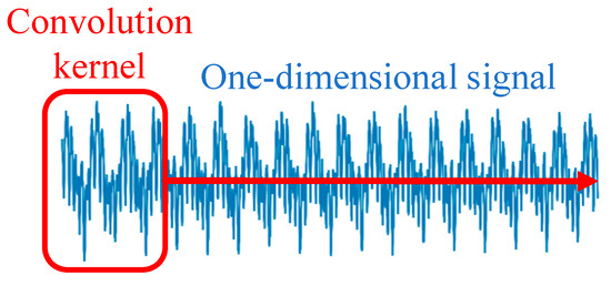
Figure 1. One-dimensional convolution extraction feature diagram.

The 1D convolution operation for a 1D input signal can be described as follows:

$$y[i]=x[i]\times k[i]={\displaystyle \sum _{j=-M}^{M}x}[i-j]\times k[j]$$

(1)

where $y[i]$ describes the convolution operation output, $M$ indicates the half-size of the convolution kernel, $x[i]$ describes a 1D signal (i is the time step), and $k[j]$ is the convolution kernel ($j$ is a position in the convolution kernel).

A convolution operation is usually followed by applying an activation function ReLu to introduce nonlinearity:

$$a[i]=\max (0,y[i])$$

(2)

where $a[i]$ indicates the output after applying the activation function.

(2)

Pooling layer

Pooling layers are often employed in 1D-CNNs to alleviate the features’ dimension and the computational cost while retaining the main feature information. The selected maximum pooling operation reduces the data dimension by selecting the maximum value within a specific window size. Maximum pooling can be described as follows:

$$p[j]=\max (a[i]), \mathrm{for} i\in [j\times s, j\times s+f]$$

(3)

where $p[j]$ indicates the pooling layer output; $s$ describes the step size, indicating the distance that the pooling window moves in the sequence; and $f$ indicates the size of the pooling window. Maximum pooling selects the maximum value in the window as its representation.

(3)

Fully connected layer

The fully connected layer is placed at the end of the 1D-CNN, which helps the network synthesize multi-dimensional features from different sensors (such as vibration, sound, current, and cutting forces). Its operation can be described as follows:

$$y=Wp[j]+b$$

(4)

where $y$ indicates the fully connected layer output, $W$ describes the weight matrix, and $b$ is a bias vector. Compared to traditional feature engineering methods, a 1D-CNN reduces the reliance on expert knowledge and the need for manual data pre-processing. Additionally, the pooling layer in a 1D-CNN reduces the dimension of features, thus reducing the computational cost while preserving critical information. This makes 1D-CNNs efficient and effective when processing tool wear data with complex time dependence.

2.2. Time Convolutional Network

Since RNN often faces gradient disappearing or explosion when dealing with long sequence data, it is difficult for the network to learn and retain long-term dependent information. Although RNN variants, such as LSTM [25] and GRU [26], can better handle long-term dependencies, they are still confined by inherently handling serialized data. Therefore, TCN is adopted for time series long-term dependency modeling because it can deal with long-term data dependency problems. TCN [27] employs causal convolution to make predictions dependent on past and current information, but not future data. This is particularly important in time series forecasting, where future data are unavailable in real-world scenarios. By stacking multiple convolutional layers and using dilated convolution, TCN effectively increases its receptive field, i.e., the range of historical data that the model can “see”. This allows the TCN to capture long-term data dependencies without significantly increasing the computational costs. Compared with RNNs, such as LSTM or GRU, the convolutional operations of TCN can be more efficiently computed in parallel because the forward propagation of the convolutional network does not depend on the previous point in time in the sequence. This improves the efficiency of the TCN when dealing with large-scale data. The TCN mainly comprises the causal, dilated, and residual convolutions.

(1)

Causal convolution

The main idea of causal convolution is to make the prediction dependent only on the previous and current information in the time series analysis. This is achieved by controlling the interaction of the convolution kernel with the input data. For a 1D input sequence $x[t]$, where t is the time step, causal convolution is described as follows:

$$y[t]={\displaystyle \sum _{s=0}^{s-1}x}[t-s]\cdot k[s]$$

(5)

where $y[t]$ describes the convolution output at time $t$,$k[s]$ is the convolution kernel, and $s$ is the convolution kernel index.

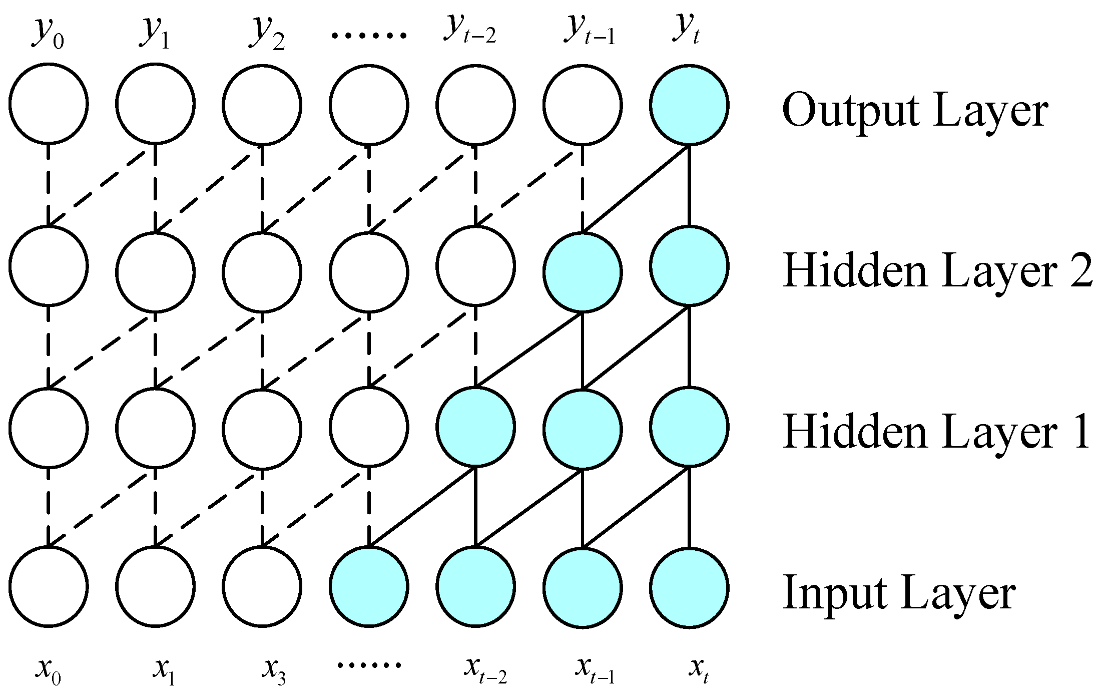
As presented in Figure 2, considering that the input layer’s last two nodes are $x_{t-1}$ and $x_t$, the calculated output at time $t$ is $y_t$, which is obtained as follows:

$$y_t=k_0\times x_t+k_1\times x_{t-1}$$

(6)

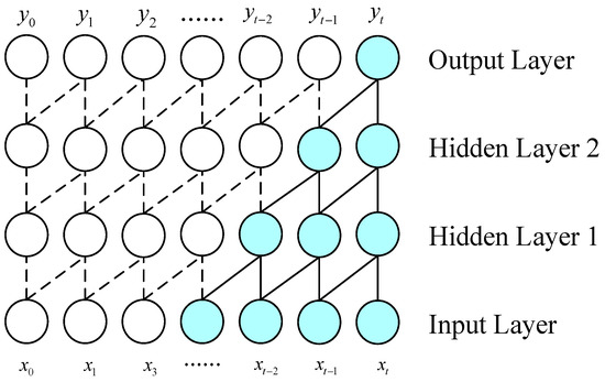
Figure 2. The causal convolution structure’s schematic diagram.

(2)

Dilated convolution

Simple causal convolution faces the conventional CNN issue; that is, the modeling length of time is confined by the convolution kernel size [28]. In order to grasp a longer dependency, it is necessary to stack many layers linearly. Therefore, the TCN usually employs dilatation convolution to handle long-term dependencies in the time series data while maintaining the model’s causality, as shown in Figure 3.

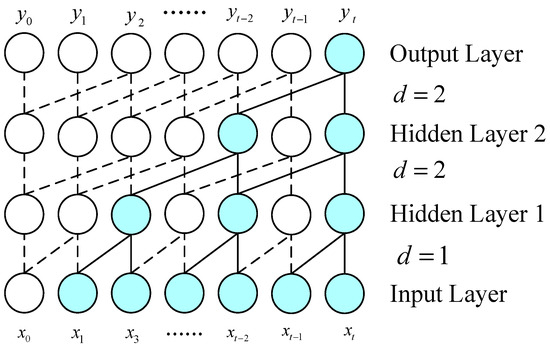
Figure 3. Dilated causal convolution structure diagram.

Dilated convolution introduces intervals inside the convolution kernel to cover longer input sequences. This allows the network to “see” and process further historical information, capturing long-term dependencies without increasing the convolution kernel size or the number of network layers [29]. The following relation describes the dilated convolution:

$$y[t]={\displaystyle \sum _{s=0}^{s-1}x}[t-s\cdot d]\cdot k[s]$$

(7)

where $d$ is the dilated factor, determining how the convolution kernel covers the input data. The more significant the $d$ value, the more input data points the convolution kernel “skips”, allowing the network to cover a longer input sequence.

(3)

Residual connections

Residual connections in the TCN improve the network’s learning ability, especially when dealing with deep networks. Residual connections help solve gradient disappearing in deep networks and enhance information transmission by introducing feeder lines from the previous layer to the next.

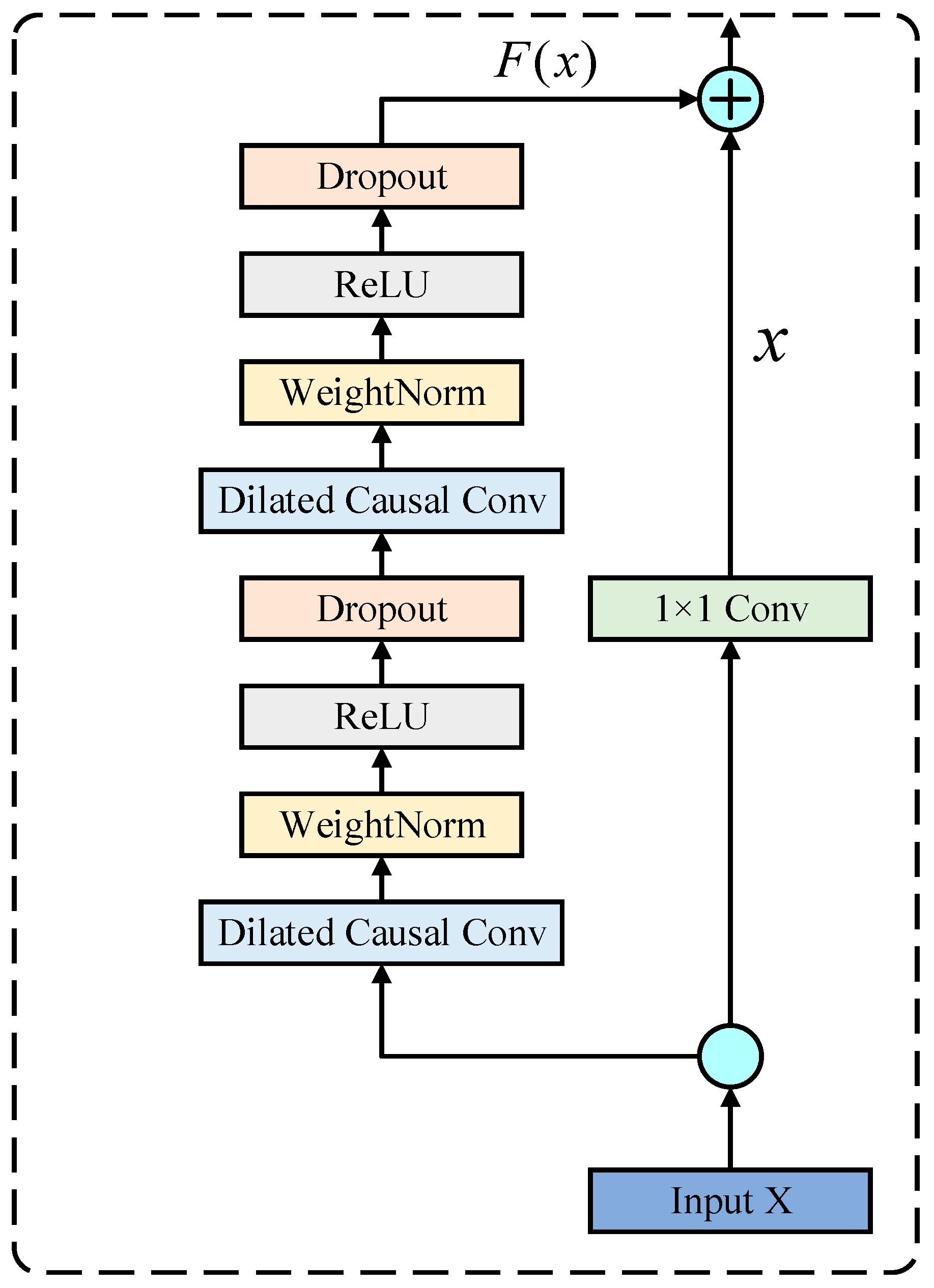
As described in Figure 4, assuming that the input of a convolution block in a TCN is $x$, and the output after applying the convolution is $F(x)$, the residual connections’ output is described as follows:

$$O(x)=Activation(x+F(x))$$

(8)

Figure 4. The TCN residual structure’s schematic diagram.

Applying the residual connection to the TCN improves the model’s capability to process long-term dependency and complex time series data, especially the residual structure, which is particularly important in deep network construction. This improves the efficiency and reliability of the TCN for prediction tasks for many complex time series.

3. Proposed Model

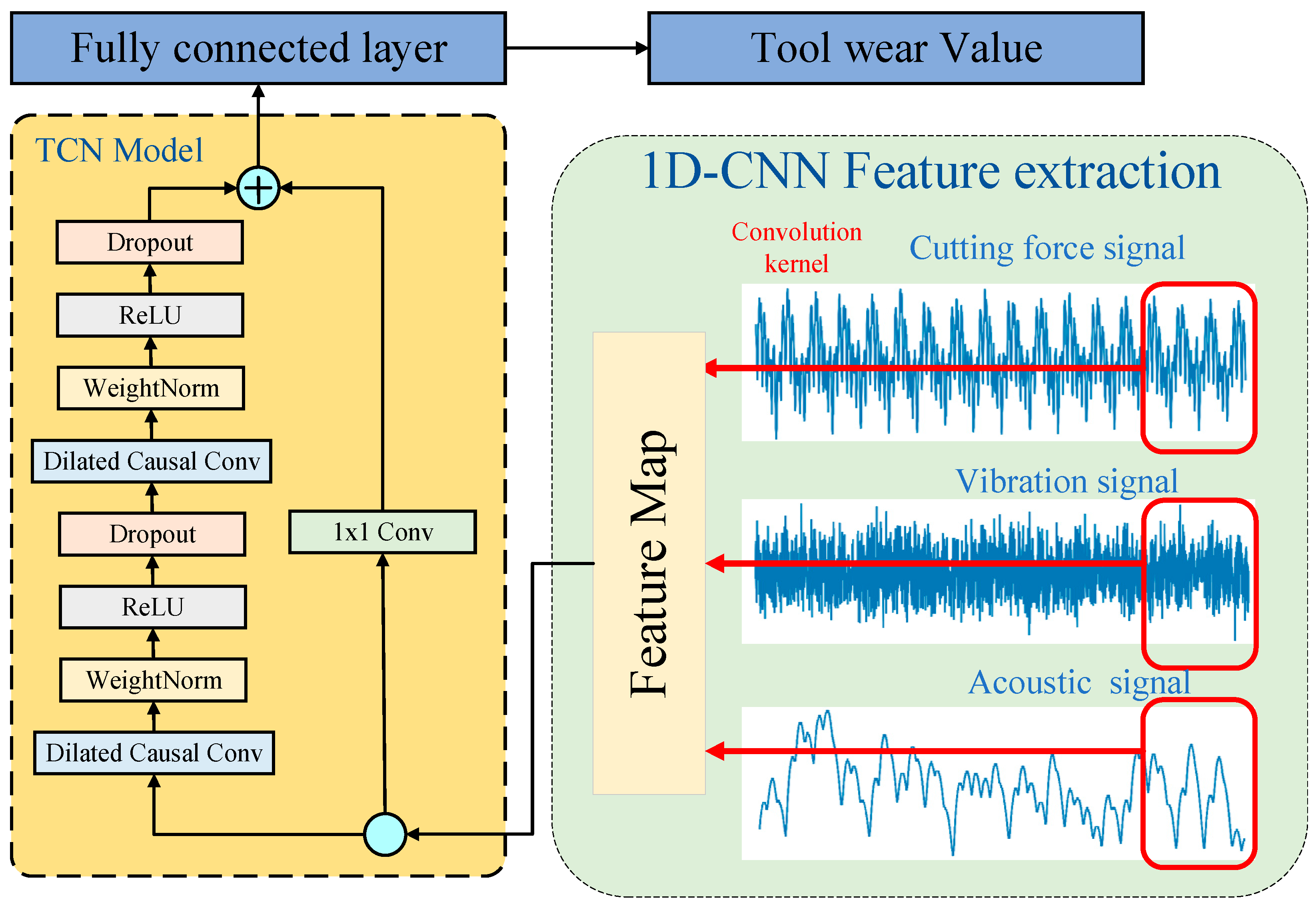
Tool wear is a complex process that considerably affects the production efficiency and quality during manufacturing. Tool wear monitoring and management are crucial for efficient, high-quality production. However, since tool wear cannot be predicted immediately in the machining procedure, sensors are utilized to monitor the cutting force, vibration, acoustic emission, and other signals in the machining procedure to forecast tool wear indirectly. In order to meet the tool wear prediction’s precision and real-time requirements, a CTCN model is established using the 1D-CNN and TCN. Figure 5 shows the structure and prediction flow based on the CTCN model.

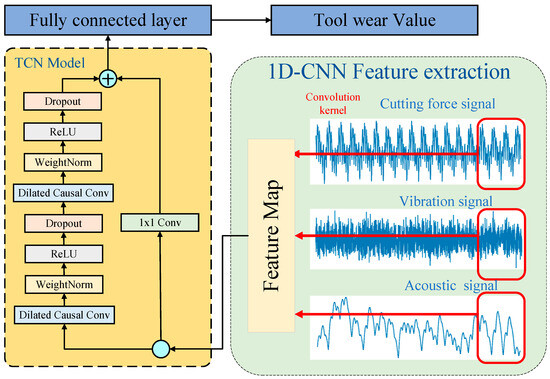
Figure 5. CTCN model network structure diagram.

(1)

A multi-channel 1D-CNN extracts features from the time series signals gathered using the sensor. Subsequently, the multi-feature integration is achieved by combining the feature maps derived from various convolution branches.

(2)

The extracted features in step (1) are fed into the TCN network for long-term dependency modeling to learn time series features corresponding to tool wear features.

(3)

In the end, a mapping relation between high-dimensional features and tool wear values is established through the fully connected layer to realize tool wear prediction.

4. Experimental Study

4.1. Dataset

In order to evaluate the established CTCN’s effectiveness, the PHM2010 tool wear dataset was adopted for verification [30]. The PHM2010 tool wear dataset can be downloaded from https://phmsociety.org/phm_competition/2010-phm-society-conference-data-challenge/ (accessed on 1 December 2023). Figure 6 presents the PHM2010 data experimental setup. Under dry milling conditions, a high-speed CNC machine tool was utilized to test a three-edge ball-end mill with stainless steel (HRC-52) as the workpiece material. The spindle speed was 10,400 RPM, the sampling frequency was 50 KHz, the feed speed was 1555 mm/min, and the Z-axis and Y-axis cutting depths were 0.2 mm and 0.125 mm, respectively.

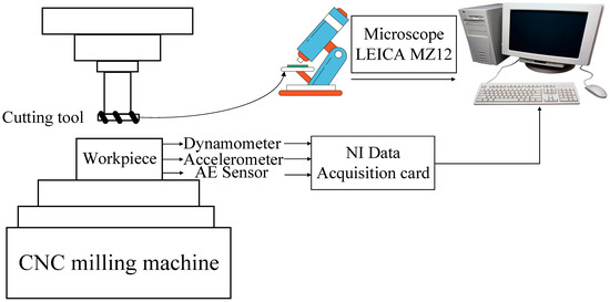
Figure 6. The experimental apparatus’s PHM schematic diagram.

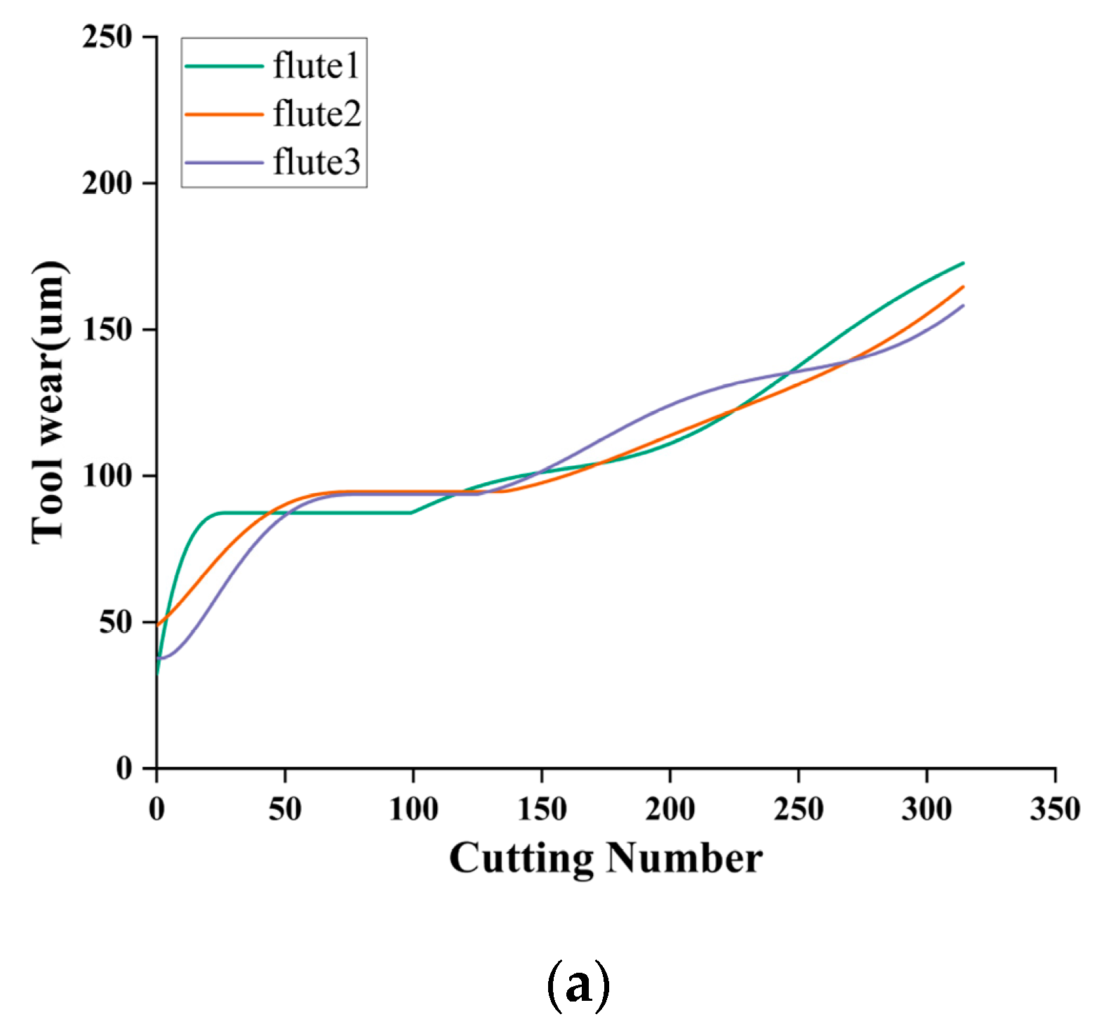
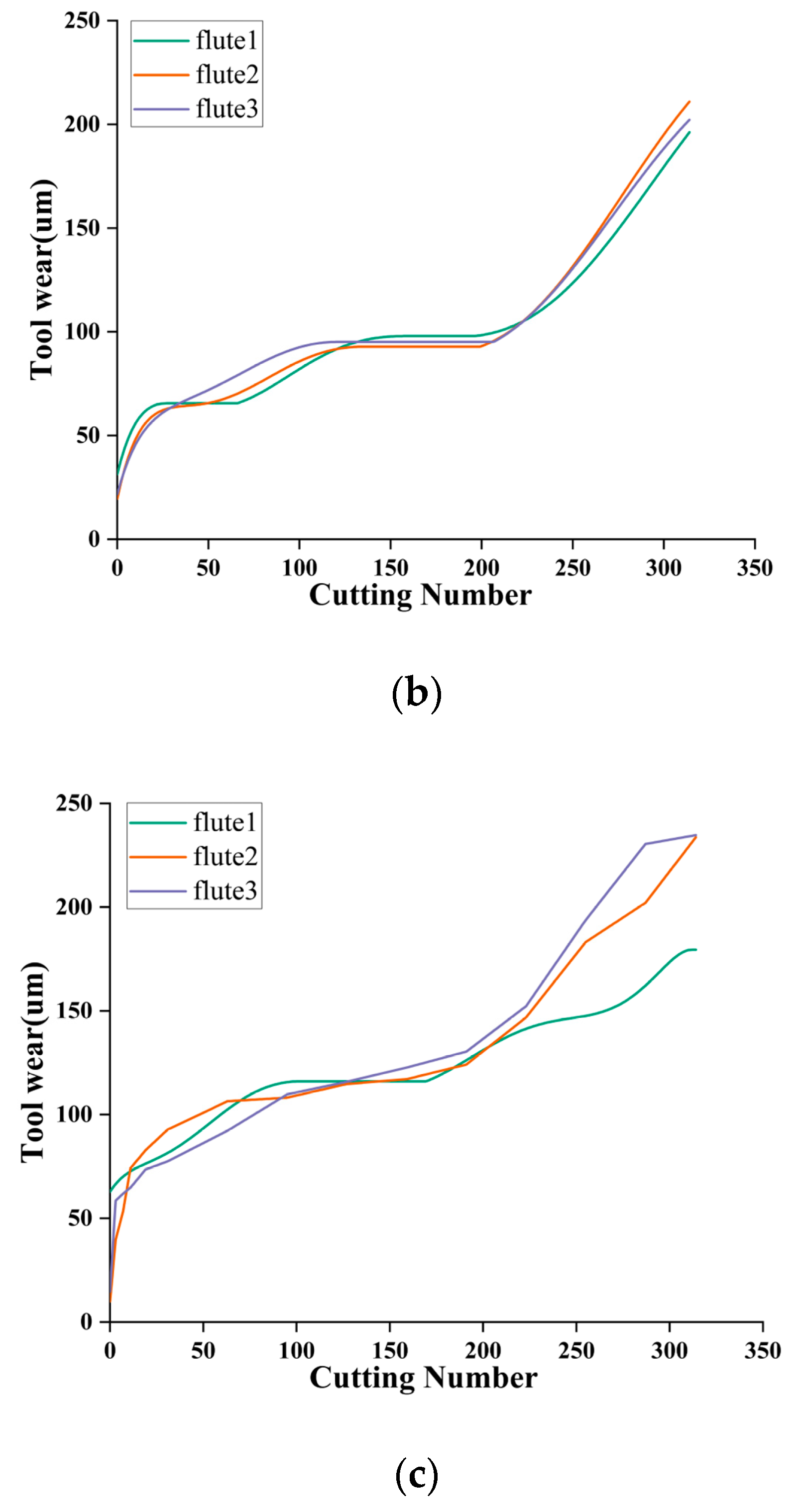
Table 1 shows the test equipment. The tool was milled along the X-axis direction during the test and removed after each milling. After each milling operation, the tool wear behind the three cutters was measured using a LEICA MZ12 microscope, recorded as flute1–3, and the wear measurement accuracy was 10⁻³ mm. Finally, a total of three cutters were tested under the same experimental conditions, designated C1, C4, and C6, and 315 cutting tests were performed on each cutter. Finally, 315 datasets and the corresponding wear values of three blades were collected for each cutter. The C1, C4, and C6 datasets recorded the full life cycle of the cutter wear. Figure 7 shows the trend of the three-blade wear for each cutter. For safety reasons, the maximum value of the three blades is chosen as the final wear label.

Table 1. Model of the experimental equipment.

Equipment	Type
CNC milling machine	Roders Tech RFM760
Dynamometer	Kistler 9265B
Charge amplifier	Kistler 5019A
Acoustic emission sensor	Kistler AE sensor
Cutters	3-flute ball carbide milling cutters
Data acquisition card	DAQ NI PCI 1200
Abrasion measuring apparatus	LEICA MZ12 microscope

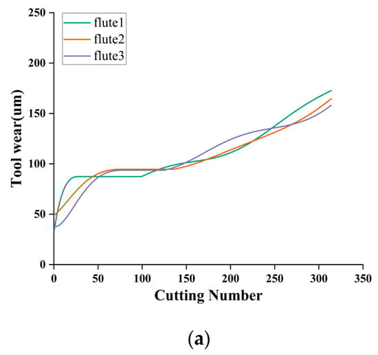
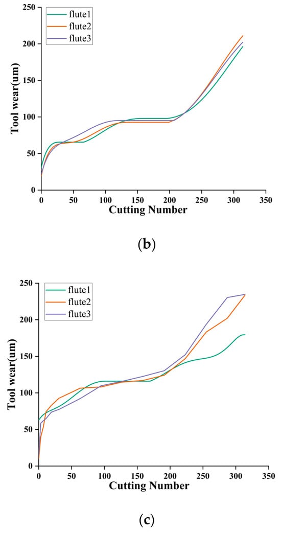
Figure 7. The PHM2010 dataset’s tool wear value curves: (a) C1 tool wear value curve, (b) C4 tool wear value curve, and (c) C6 tool wear value curve.

4.2. Data Study and Preprocessing

During the tool wear experiment, each experiment covers three stages: tool feed, stable cutting, and tool retraction. Since the signal is relatively stable in the stable cutting stage, the signal collected from the tool can effectively reflect the degree of tool wear. As presented in Figure 8, the generated signals often need clarification during the tool feed and retraction stages. They cannot accurately represent the relation between the tool wear and the signal. Therefore, the unstable signal points of 3% before and after the start and end of each cut were excluded to enhance the data quality and the accuracy of the analysis. Considering the difference in the data scale between the original signals, this study adopted the Z-Score normalization to standardize the signal data to alleviate the effect of various signal scales. This step creates data with a uniform scale and distribution before entering the network model, thus improving the consistency and accuracy of the model when processing different signals.

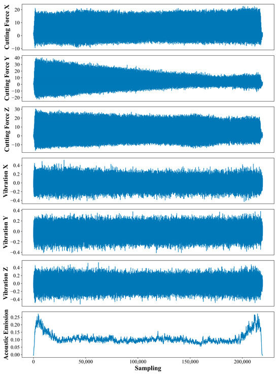
Figure 8. PHM dataset experimental process signal diagram.

4.3. Experimental Setup

Under the PyTorch framework, the CTCN model was programmed, and the NVIDIA GeForce RTX 3090 GPU was utilized to perform the learning process. The CTCN model was trained for 100 rounds, and the learning rate was chosen as 0.0001. In order to enhance the model’s generalization ability, L2 regularization terms were incorporated into the training process. Additionally, the Adam optimizer, which adjusts and optimizes the parameters through a backpropagation mechanism, was employed to minimize the loss effectively.

4.4. Evaluation Index

The evaluation index can assess the model performance. In order to assess the CTCN model’s correlation efficiency, the mean absolute error (MAE), root mean square error (RMSE), determination coefficient ($R^2$), and mean absolute percentage error (MAPE) were selected as assessment indices, as shown in Equations (9)–(12). The MAE is the average of the absolute error between the predicted and actual values. The RMSE is the square root of the MSE, providing an error measure on the same scale as the actual value. $R^2$ measures the ability of the model to describe the variables, i.e., how well the model fits the data. A value of $R^2$ closer to 1 reveals the better fitting of the model. The MAPE is the magnitude of the prediction error relative to the actual value. It calculates the mean ratio of the absolute value of the difference between the predicted and actual values to the actual one.

$$\mathrm{MAE}=\frac{1}{n}{\displaystyle \sum _{i=1}^n|}{y}_i-{\widehat{y}}_i|$$

(9)

$$\mathrm{RMSE}=\sqrt{\frac{1}{n}{\displaystyle \sum _{i=1}^n{(y_i-{\widehat{y}}_i)}^2}}$$

(10)

$$R^2=1-\frac{{\displaystyle \sum _{i=1}^n{(y_i-{\widehat{y}}_i)}^2}}{{\displaystyle \sum _{i=1}^n{(y_i-\overline{y})}^2}}$$

(11)

$$\mathrm{MAPE}=\frac{100\%}{n}{\displaystyle \sum _{i=1}^n\left|\frac{y_i-{\widehat{y}}_i}{y_i}\right|}$$

(12)

where $n$ indicates the number of samples, and $y_i$ and ${\widehat{y}}_i$ describe the actual and predicted values of the ith sample, respectively.

4.5. Experimental Setup and Model Parameter Adjustment

The current test was performed using the PHM tool wear dataset, and the cross-validation strategy outlined in Table 2 was employed for model training and evaluation. The experiment process was divided into three groups, each adopting training and testing stages.

Table 2. Training and testing set settings.

Training Set		Testing Set
c4	c6	c1
c1	c6	c4
c1	c4	c6

This experiment established the CTCN model using the model parameters presented in Table 3. The model’s parameters can be calculated as shown below.

Table 3. CTCN model parameters.

Layer	Kernel Shape	Output Shape
Layer1.CNN.Conv1d	[7, 64, 9]	[32, 64, 1024]
Layer2.CNNConv1d	[64, 64, 5]	[32, 64, 512]
Layer3.CNN.Conv1d	[64, 128, 3]	[32, 128, 258]
Layer4.TCN.Conv1d	/	[32, 7, 130]
Layer5.TCN.Chomp1d	/	[32, 7, 129]
Layer6.TCN.Conv1d	/	[32, 1024, 129]
Layer7.TCN.Chomp1d	/	[32, 1024, 129]
Layer8.Linear	[1024, 1]	[32, 129, 1]

4.6. Experimental Results and Discussion

4.6.1. Experimental Results

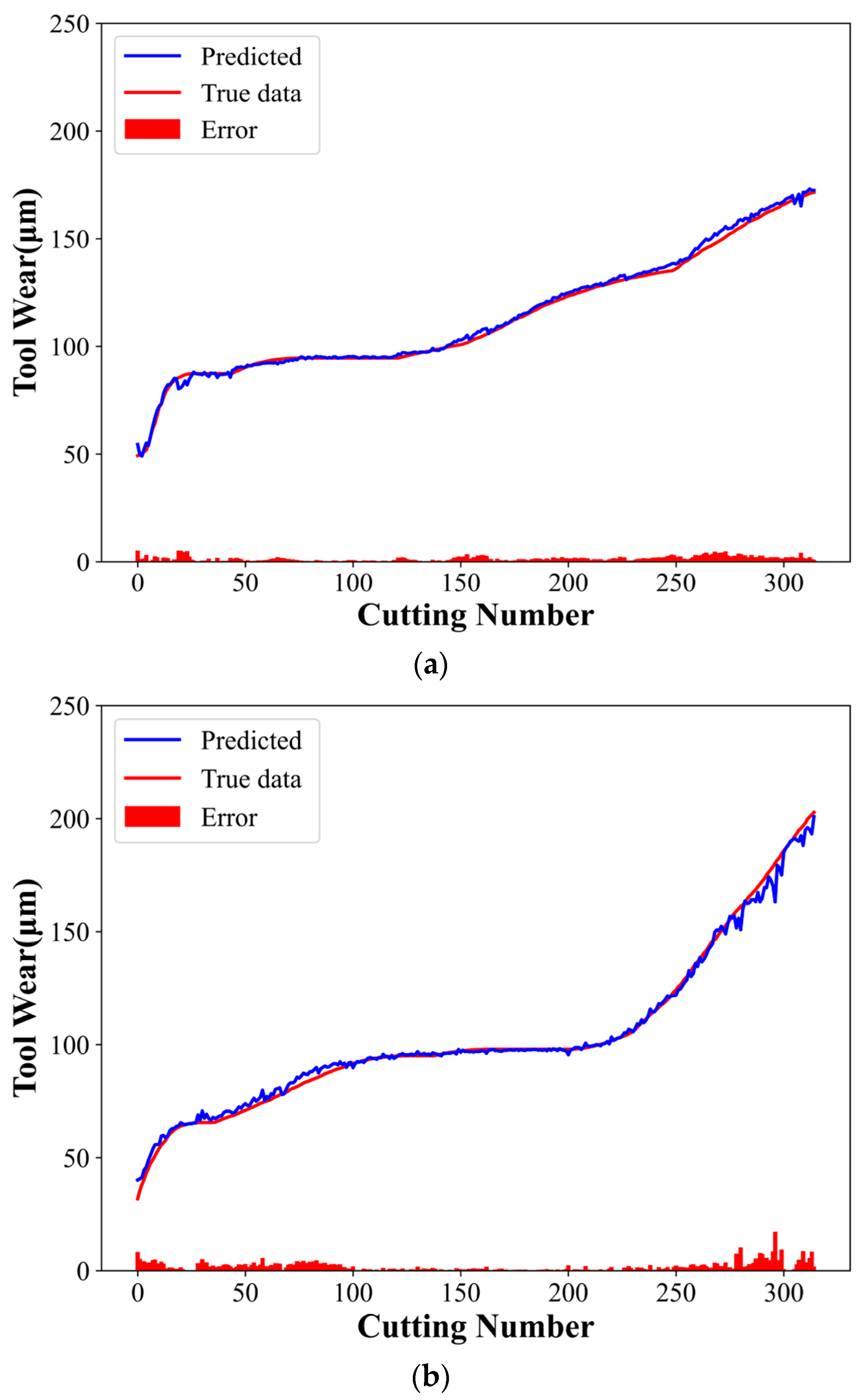
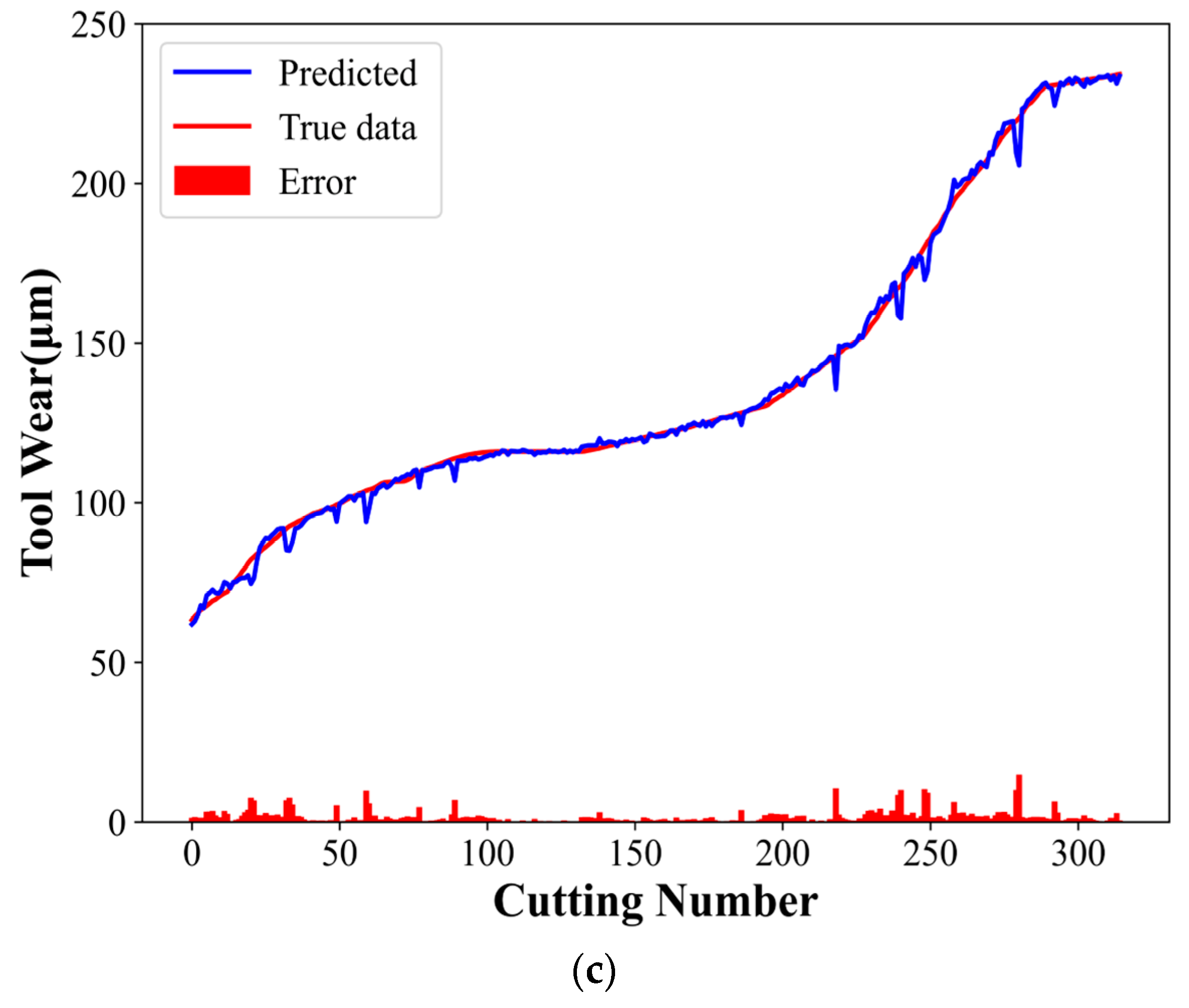
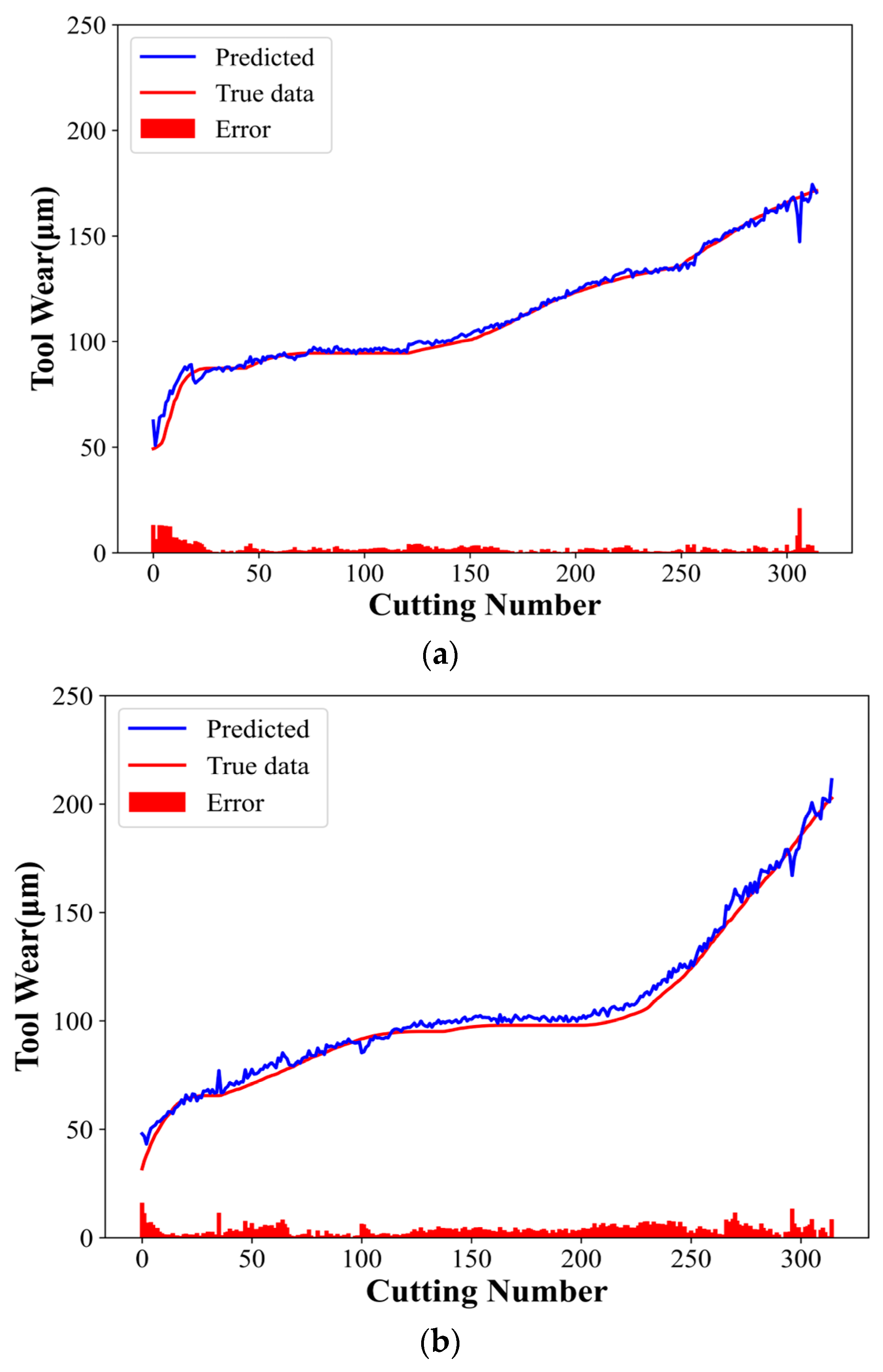
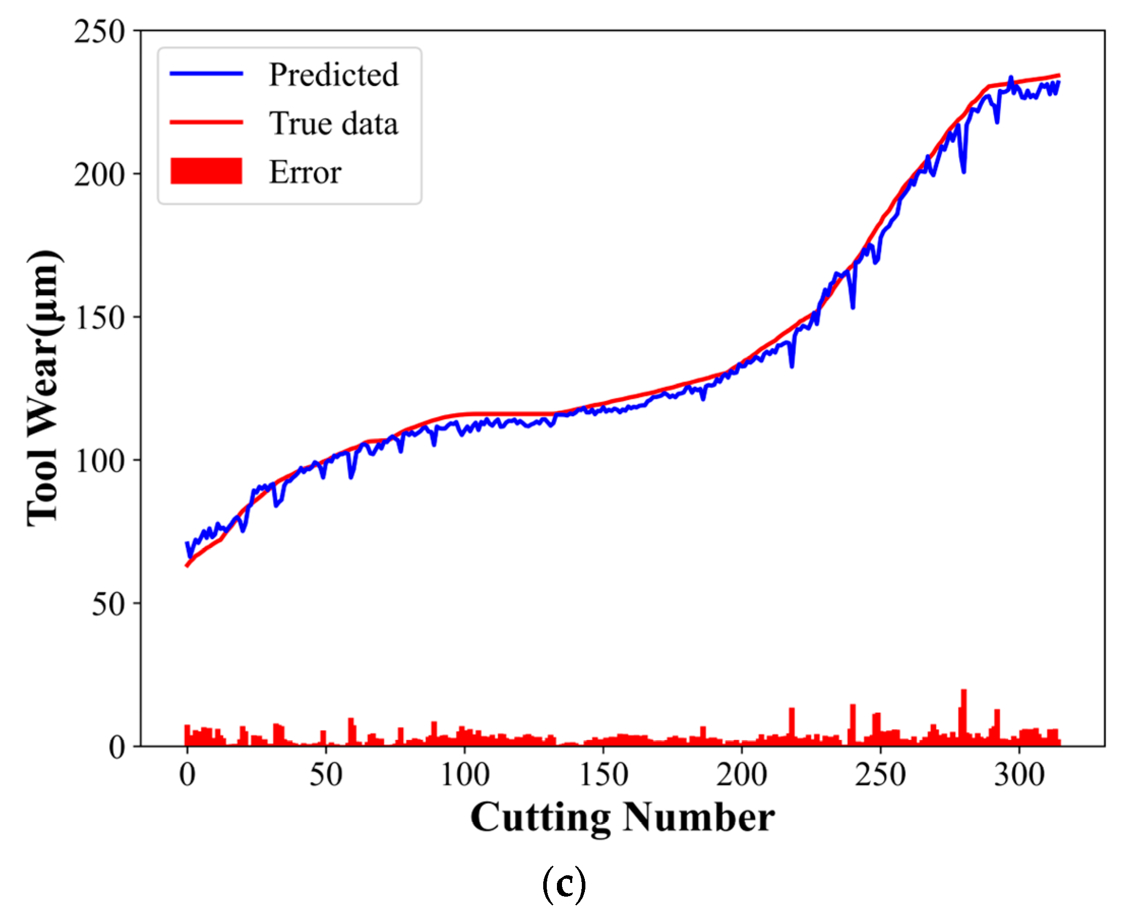
Figure 9 shows the experimental results, where the predicted and actual tool wear curves are indicated in blue and red, respectively, and the red histogram represents their difference. The experimental results indicate the compatibility of the predicted curve with the actual curve. Table 4 shows the evaluation indices corresponding to the three groups of experiments.

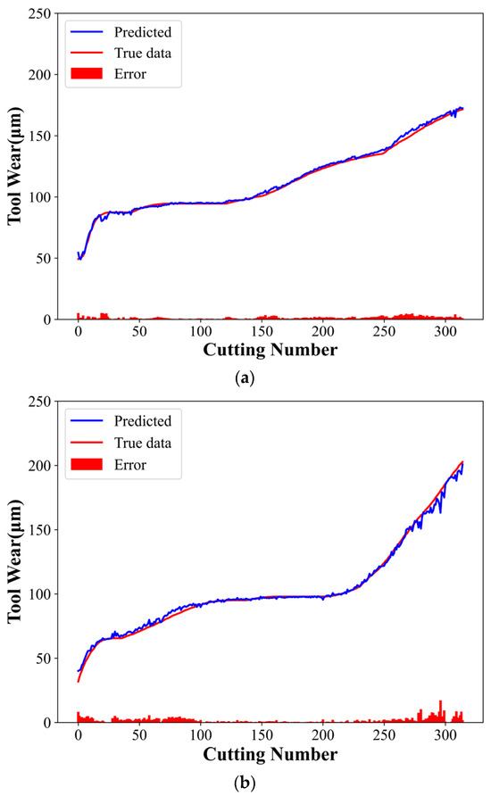
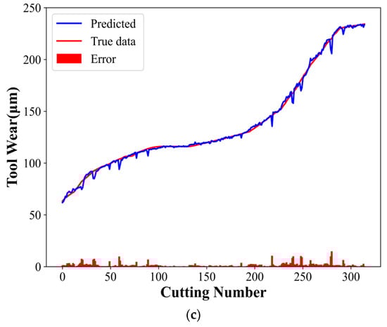
Figure 9. CTCN model experimental results: (a) C1 tool predicted wear, (b) C4 tool predicted wear, and (c) C6 tool predicted wear.

Table 4. Ablation results.

Models	Datasets
	C1				C4				C6
	MAE	RMSE	R2	MAPE	MAE	RMSE	R2	MAPE	MAE	RMSE	R2	MAPE
CNN	3.609	6.476	0.946	0.035	5.201	8.131	0.955	0.052	4.423	6.388	0.981	0.033
TCN	2.551	5.198	0.965	0.024	5.273	8.729	0.942	0.048	6.834	9.271	0.961	0.047
CTCN	2.031	3.553	0.983	0.019	2.744	6.151	0.974	0.027	2.415	4.274	0.991	0.018

4.6.2. Ablation Experiment

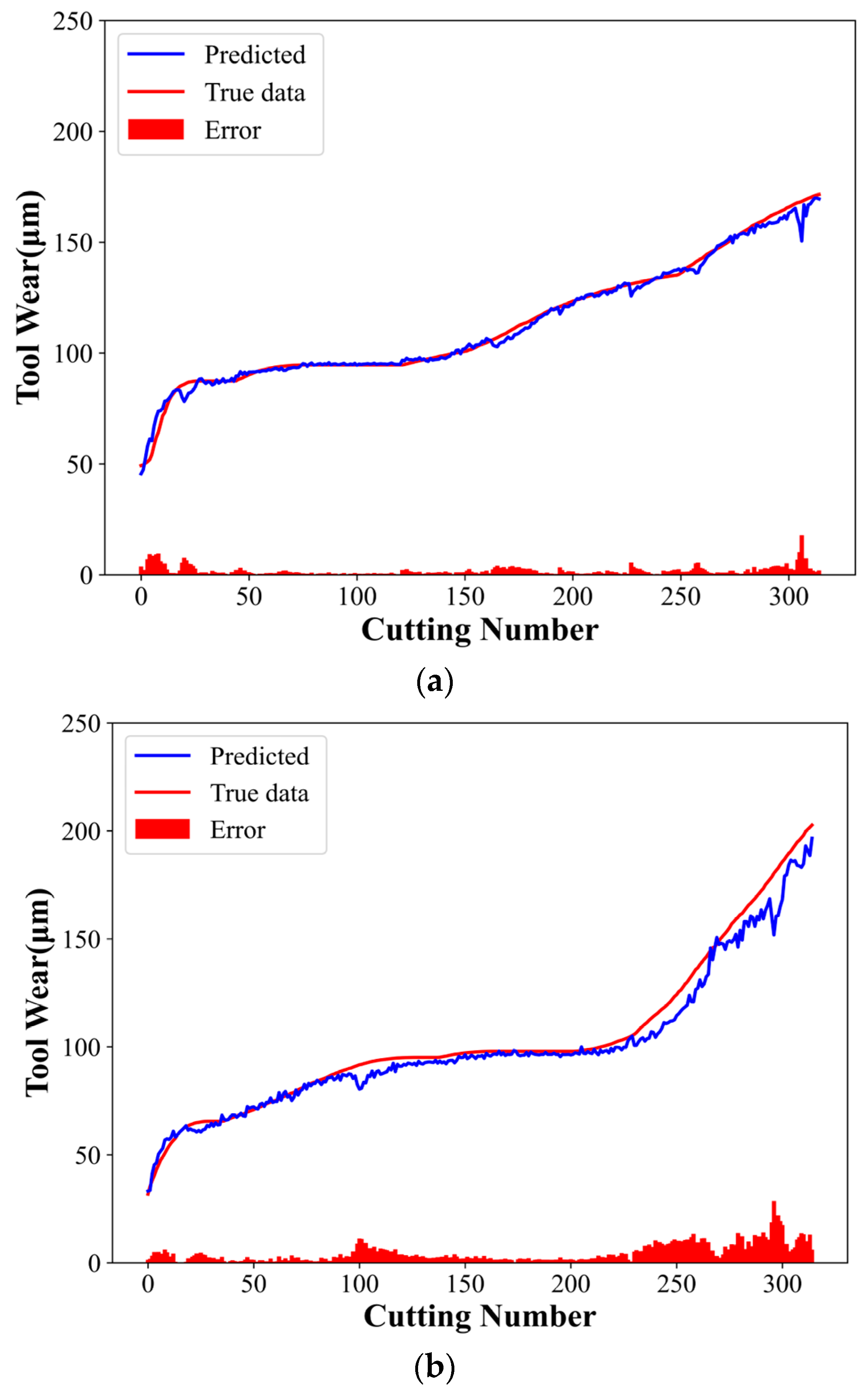
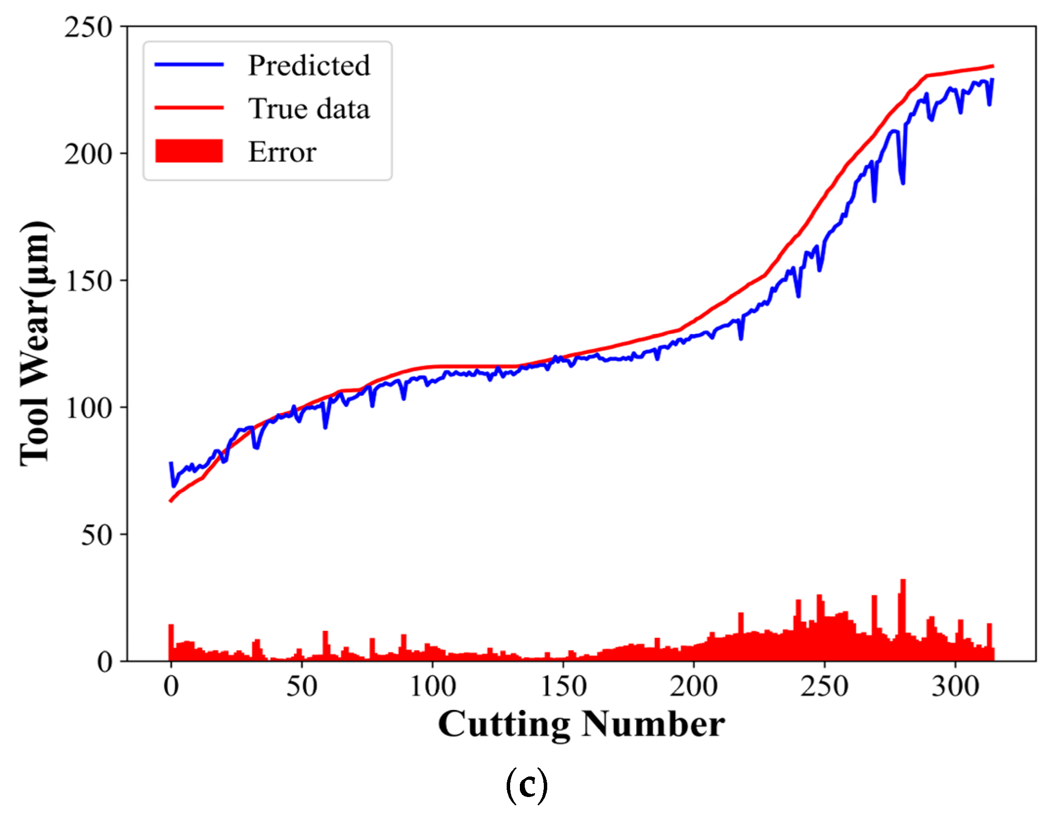
The ablation experiments were designed to demonstrate the model’s effectiveness and superiority. Experiments 1 and 2 employed the CNN and TCN models, respectively, with the same parameters as the CTCN model. Figure 10 and Figure 11 present the experimental results of the CNN and TCN models, respectively. Table 4 shows the evaluation indices for different models.

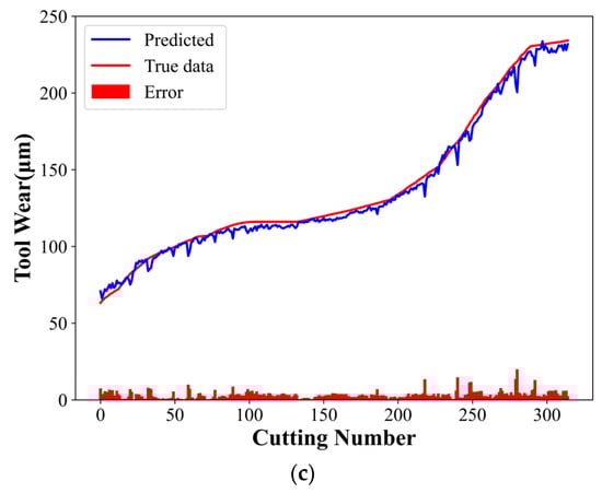
Figure 10. CNN model experimental results: (a) C1 tool predicted wear, (b) C4 tool predicted wear, and (c) C6 tool predicted wear.

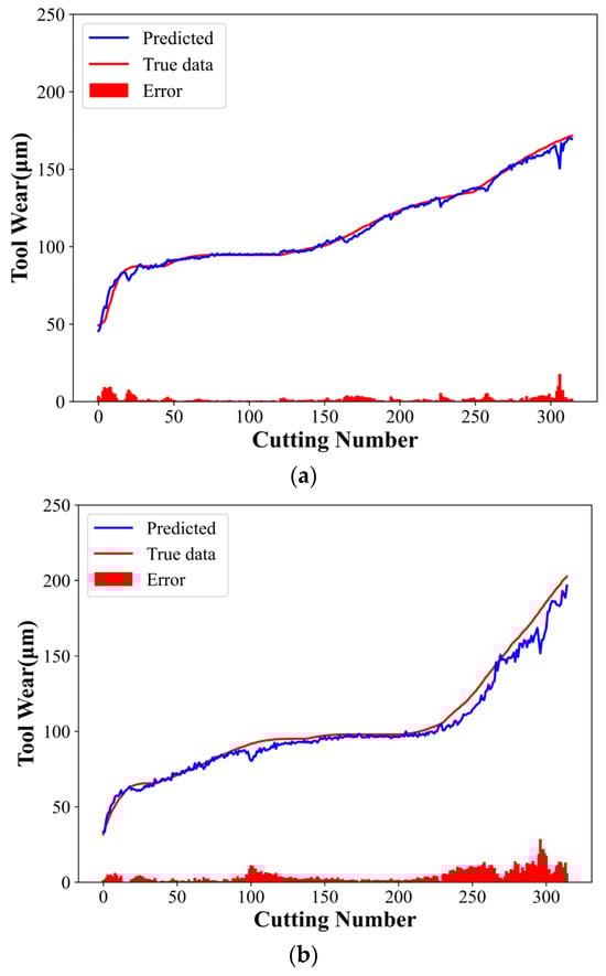
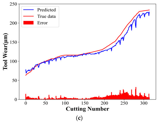
Figure 11. TCN model experimental results: (a) C1 tool predicted wear, (b) C4 tool predicted wear, and (c) C6 tool predicted wear.

The MAE, RMSE, and MAPE values of the CTCN model were lower than those of the other comparison models. In contrast, the R² values were higher than those of the comparison models in a similar group, reaching 98.38%, 97.48%, and 99.17%, respectively. The CNN mainly extracts local features from multi-channel sensor data. Additionally, its powerful spatial feature extraction capability helps the model identify and capture critical patterns during tool wear. These characteristics are crucial to understand and predict the tool wear process and are essential for the subsequent time series analysis.

The CNN-extracted features are then input into the TCN. The TCN can deal with the time dependence of these features, considering the tool wear process’s time-varying behavior. The dilated causal convolution structure of the TCN helps the model capture long-term time series dependencies without losing causality. Accordingly, the model can make accurate wear predictions based on current and historical data and reveal the wear development trend.

The established model can effectively take advantage of the sensor data’s spatial properties (captured using a CNN) and temporal properties (processed using a TCN). The ablation experiments show that combining a TCN with a CNN significantly improves the model’s overall performance, especially the prediction accuracy and the ability to understand time-dependent relationships. This demonstrates the unique and complementary roles of CNNs and TCNs in the established model and their synergies in processing complex time series data.

4.6.3. Model Comparison

Since the PHM2010 tool wear dataset has become the benchmark dataset for many relevant scholars to perform experiments, several models using the PHM2010 dataset were selected for comparison to demonstrate the CTCN model’s superiority. Table 5 presents the relevant assessment indices of various models under the PHM2010 dataset.

Table 5. Comparison results of different models.

Models	Datasets
	C1				C4				C6
	MAE	RMSE	R2	MAPE	MAE	RMSE	R2	MAPE	MAE	RMSE	R2	MAPE
SSAE-BP [31]	12.00	13.53	0.91	/	12.44	14.62	0.93	/	7.29	10.08	0.94	/
Parallel-CNN [32]	3.89	5.54	/	/	4.53	5.27	/	/	3.52	4.90	/	/
CBLSTM [33]	7.5	10.8	/	/	6.1	7.1	/	/	8.1	9.8	/	/
PGGM [34]	4.3	5.0	/	/	8	9.6	/	/	5.9	13.9	/	/
MFPBM [35]	4.2	4.9	/	/	5.8	7.1	/	/	4.4	5.8	/	/
PRes–SBiLSTM [36]	4.7	8.5	/	/	5.6	7.9	/	/	4.7	5.9	/	/
CGRU [37]	3.32	5.33	0.962	/	4.95	7.43	0.962	/	4.45	6.47	0.974	/
CTCN	2.031	3.553	0.983	0.019	2.744	6.151	0.974	0.027	2.415	4.274	0.991	0.018

After a comprehensive performance comparison using the same dataset, the results indicate the superiority of the established model to other models in each evaluation index. This highlights the advantage of the established model in understanding and analyzing tool wear data, especially when dealing with complex data structures and variable data characteristics. Due to its unique algorithm design and efficient data processing strategy, this model stands out in competitive comparisons, demonstrating its potential in practical applications.

5. Conclusions

The current work combines multi-channel 1D-CNN with TCN models to establish a tool wear prediction model and verifies the tool wear prediction capability of the CTCN model. The model performs excellently in various evaluation indices, such as RMSE and MAPE. Compared with existing forecasting models, the established model provides higher precision and stability when dealing with complex datasets. The model outperforms the single CNN or TCN model in many experiments, and the following conclusions can be obtained:

(1)

A 1D-CNN can effectively extract the 1D signal features, which can efficiently describe the tool wear state.

(2)

Due to the dilated causal convolution structure of the TCN, long-term time series dependencies can be effectively captured without losing causality. Accordingly, the model can make accurate wear predictions based on current and historical data and reveal the development trend.

(3)

This study demonstrates that combining a CNN and TCN can significantly improve tool wear prediction. A CNN’s powerful feature extraction ability, combined with the efficient time series analysis of a TCN, helps the model effectively capture complex tool wear patterns.

The training and testing datasets for the CTCN model were specifically tailored to the conditions and environment of high-speed milling machining obtained from high-speed CNC machining centers. Therefore, the applicability of the CTCN model in tool wear prediction is mainly limited to similar high-speed milling scenarios such as those in the training data environment. Due to different mechanical properties, cutting parameters, and operating conditions in turning and grinding machining processes, these variations may degrade the tool wear prediction by the CTCN model in these scenarios. Since each machining method exhibits unique tool wear patterns and influencing factors, training and adapting the model using specific datasets from each machining process are necessary to enhance its prediction accuracy and generalization ability. Consequently, although the CTCN model may provide an excellent tool wear prediction for high-speed CNC milling machining, its predictive capability might be constrained when applied to other scenarios, such as turning and grinding. Further customization and optimization are necessary to adapt to these scenarios’ specific requirements and conditions.

In future work, we will apply our model to larger and more diverse datasets, further validating its generalization and robustness, especially in different manufacturing environments and with more varied tool wear. Additionally, the model interpretation should be improved. As a future work, the interpretability of the model should be enhanced so that users can better understand the internal logic of the model’s predictions.

References

- Xia, W.; Zhou, J.; Jia, W.; Guo, M. Milling Tool Wear Prediction Based on 1DCNN-LSTM. In Proceedings of the 8th International Conference on Mechanical, Automotive and Materials Engineering, Hanoi, Vietnam, 16–18 December 2022; Springer: Berlin/Heidelberg, Germany, 2022; pp. 77–91. [Google Scholar]
- Knittel, D.; Nouari, M. Milling diagnosis using machine learning approaches. In Proceedings of the Surveillance, Vishno and AVE Conferences 2019, Lyon, France, 8–10 July 2019. [Google Scholar]
- Zhou, L. Performance of Cellular-Based Positioning with Machine Learning (Dissertation). 2022. Available online: https://urn.kb.se/resolve?urn=urn:nbn:se:kth:diva-320524 (accessed on 1 December 2023).
- Liang, X.; Liu, Z.; Wang, B. State-of-the-art of surface integrity induced by tool wear effects in machining process of titanium and nickel alloys: A review. Measurement 2019, 132, 150–181. [Google Scholar] [CrossRef]
- Dantone, M.; Gall, J.; Fanelli, G.; Van Gool, L. Real-time facial feature detection using conditional regression forests. In Proceedings of the 2012 IEEE Conference on Computer Vision and Pattern Recognition, Providence, RI, USA, 16–21 June 2012; pp. 2578–2585. [Google Scholar]
- Alonso, F.J.; Salgado, D.R. Analysis of the structure of vibration signals for tool wear detection. Mech. Syst. Signal Process. 2008, 22, 735–748. [Google Scholar] [CrossRef]
- Zhou, Y.; Sun, B.; Sun, W.; Lei, Z. Tool wear condition monitoring based on a two-layer angle kernel extreme learning machine using sound sensor for milling process. J. Intell. Manuf. 2022, 33, 247–258. [Google Scholar] [CrossRef]
- He, Z.; Shi, T.; Xuan, J.; Li, T. Research on tool wear prediction based on temperature signals and deep learning. Wear 2021, 478, 203902. [Google Scholar] [CrossRef]
- Ma, W.; Liu, X.; Yue, C.; Wang, L.; Liang, S.Y. Multi-scale one-dimensional convolution tool wear monitoring based on multi-model fusion learning skills. J. Manuf. Syst. 2023, 70, 69–98. [Google Scholar] [CrossRef]
- Li, C.; Zhao, X.; Cao, H.; Li, L.; Chen, X. A data and knowledge-driven cutting parameter adaptive optimization method considering dynamic tool wear. Robot. Comput.-Integr. Manuf. 2023, 81, 102491. [Google Scholar] [CrossRef]
- Gomes, M.C.; Brito, L.C.; Da Silva, M.B.; Duarte, M.A.V. Tool wear monitoring in micromilling using support vector machine with vibration and sound sensors. Precis. Eng. 2021, 67, 137–151. [Google Scholar] [CrossRef]
- Li, J.; Lu, J.; Chen, C.; Ma, J.; Liao, X. Tool wear state prediction based on feature-based transfer learning. Int. J. Adv. Manuf. Technol. 2021, 113, 3283–3301. [Google Scholar] [CrossRef]
- Li, G.; Wang, Y.; Wang, J.; He, J.; Huo, Y. Tool wear prediction based on multidomain feature fusion by attention-based depth-wise separable convolutional neural network in manufacturing. Int. J. Adv. Manuf. Technol. 2023, 124, 3857–3874. [Google Scholar] [CrossRef]
- Zhang, W.; Luktarhan, N.; Ding, C.; Lu, B. Android Malware Detection Using TCN with Bytecode Image. Symmetry 2021, 13, 1107. [Google Scholar] [CrossRef]
- Hu, Y.; Feng, W.; Li, W.; Yi, X.; Liu, K.; Ye, L.; Zhao, J.; Lu, X.; Zhang, R. Morphological classification method and data-driven estimation of the joint roughness coefficient by consideration of two-order asperity. Rev. Adv. Mater. Sci. 2023, 62, 20220336. [Google Scholar] [CrossRef]
- Elman, J.L. Learning and development in neural networks: The importance of starting small. Cognition 1993, 48, 71–99. [Google Scholar] [CrossRef]
- Liu, C.; Li, Y.; Li, J.; Hua, J. A meta-invariant feature space method for accurate tool wear prediction under cross conditions. IEEE Trans. Ind. Inf. 2021, 18, 922–931. [Google Scholar] [CrossRef]
- Wang, M.; Zhou, J.; Gao, J.; Li, Z.; Li, E. Milling Tool Wear Prediction Method Based on Deep Learning under Variable Working Conditions. IEEE Access 2020, 8, 140726–140735. [Google Scholar] [CrossRef]
- Chan, Y.; Kang, T.; Yang, C.; Chang, C.; Huang, S.; Tsai, Y. Tool wear prediction using convolutional bidirectional LSTM networks. J. Supercomput. 2022, 78, 810–832. [Google Scholar] [CrossRef]
- Kolář, P.; Burian, D.; Fojtů, P.; Mašek, P.; Fiala, Š.; Chládek, Š.; Petráček, P.; Švéda, J.; Rytíř, M. Indirect drill condition monitoring based on machine tool control system data. MM Sci. J. 2022, 10, 5905–5912. [Google Scholar] [CrossRef]
- Duan, J.; Zhang, X.; Shi, T. A Hybrid Attention-Based Paralleled Deep Learning model for tool wear prediction. Expert Syst. Appl. 2023, 211, 118548. [Google Scholar] [CrossRef]
- Tan, X.; Triggs, B. Enhanced local texture feature sets for face recognition under difficult lighting conditions. IEEE Trans. Image Process. 2010, 19, 1635–1650. [Google Scholar] [PubMed]
- Kiranyaz, S.; Avci, O.; Abdeljaber, O.; Ince, T.; Gabbouj, M.; Inman, D.J. 1D convolutional neural networks and applications: A survey. Mech. Syst. Signal Process. 2021, 151, 107398. [Google Scholar] [CrossRef]
- Xie, X.; Huang, M.; Liu, Y.; An, Q. Intelligent Tool-Wear Prediction Based on Informer Encoder and Bi-Directional Long Short-Term Memory. Machines 2023, 11, 94. [Google Scholar] [CrossRef]
- Hochreiter, S.; Schmidhuber, J. Long short-term memory. Neural Comput. 1997, 9, 1735–1780. [Google Scholar] [CrossRef]
- Cho, K.; Van Merriënboer, B.; Bahdanau, D.; Bengio, Y. On the properties of neural machine translation: Encoder-decoder approaches. arXiv 2014, arXiv:1409.1259. [Google Scholar]
- Bai, S.; Kolter, J.Z.; Koltun, V. An empirical evaluation of generic convolutional and recurrent networks for sequence modeling. arXiv 2018, arXiv:1803.01271. [Google Scholar]
- HKechang, H.; Jingjiao, L. Short-term Load. Forecasting Considering Demand Response. In Proceedings of the 2021 IEEE Sustainable Power and Energy Conference (iSPEC), Nanjing, China, 23–25 December 2021; pp. 2472–2476. [Google Scholar]
- Zhang, H.; Chen, Y.; Chu, X.; Zhang, Z.; Hao, T.; Wu, Z.; Yang, Y. Neural Computing for Advanced Applications. In Proceedings of the Third International Conference, NCAA 2022, Jinan, China, 8–10 July 2022; Proceedings, Part I. Springer Nature: Berlin/Heidelberg, Germany, 2022. [Google Scholar]
- Li, X.; Lim, B.S.; Zhou, J.H.; Huang, S.; Phua, S.J.; Shaw, K.C.; Er, M.J. Fuzzy neural network modelling for tool wear estimation in dry milling operation. In Proceedings of the Annual Conference of the PHM Society 2009, San Diego, CA, USA, 27 September–1 October 2009. [Google Scholar]
- Qin, Y.; Liu, X.; Yue, C.; Zhao, M.; Wei, X.; Wang, L. Tool wear identification and prediction method based on stack sparse self-coding network. J. Manuf. Syst. 2023, 68, 72–84. [Google Scholar] [CrossRef]
- Xu, X.; Wang, J.; Zhong, B.; Ming, W.; Chen, M. Deep learning-based tool wear prediction and its application for machining process using multi-scale feature fusion and channel attention mechanism. Measurement 2021, 177, 109254. [Google Scholar] [CrossRef]
- Zhao, R.; Yan, R.; Wang, J.; Mao, K. Learning to monitor machine health with convolutional bi-directional LSTM networks. Sensors 2017, 17, 273. [Google Scholar] [CrossRef]
- Wang, J.; Li, Y.; Zhao, R.; Gao, R.X. Physics guided neural network for machining tool wear prediction. J. Manuf. Syst. 2020, 57, 298–310. [Google Scholar] [CrossRef]
- Zhang, K.; Zhou, D.; Zhou, C.A.; Hu, B.; Li, G.; Liu, X.; Guo, K. Tool wear monitoring using a novel parallel BiLSTM model with multi-domain features for robotic milling Al7050-T7451 workpiece. Int. J. Adv. Manuf. Technol. 2023, 129, 1883–1899. [Google Scholar] [CrossRef]
- Liu, X.; Liu, S.; Li, X.; Zhang, B.; Yue, C.; Liang, S.Y. Intelligent tool wear monitoring based on parallel residual and stacked bidirectional long short-term memory network. J. Manuf. Syst. 2021, 60, 608–619. [Google Scholar] [CrossRef]
- Yang, J.; Wu, J.; Li, X.; Qin, X. Tool wear prediction based on parallel dual-channel adaptive feature fusion. Int. J. Adv. Manuf. Technol. 2023, 128, 145–165. [Google Scholar] [CrossRef]
Disclaimer/Publisher’s Note: The statements, opinions and data contained in all publications are solely those of the individual author(s) and contributor(s) and not of MDPI and/or the editor(s). MDPI and/or the editor(s) disclaim responsibility for any injury to people or property resulting from any ideas, methods, instructions or products referred to in the content. |
© 2024 by the authors. Licensee MDPI, Basel, Switzerland. This article is an open access article distributed under the terms and conditions of the Creative Commons Attribution (CC BY) license (https://creativecommons.org/licenses/by/4.0/).