A Rolling Bearing Fault Diagnosis Method Combining MSSSA-VMD with the Parallel Network of GASF-CNN and BiLSTM

Abstract

Once the rolling bearing fails, it will threaten the normal operation of the whole rotating machinery. Therefore, it is very necessary to conduct research on rolling bearing fault diagnosis. This paper proposes a rolling bearing fault diagnosis method combining MSSSA-VMD (variational mode decomposition optimized by the improved salp swarm algorithm based on mixed strategy) with the parallel network of GASF-CNN (convolutional neural network based on Gramian angular summation field) and bi-directional long short-term memory (BiLSTM) to solve the problem of poor diagnostic performance for the rolling bearing faults caused by the respective limitations of existing fault diagnosis methods based on signal processing and deep learning. Firstly, MSSSA-VMD is proposed to solve the problem where the decomposition effect of VMD is not ideal due to improper parameter selection. Then, MSSSA-VMD is employed to preprocess and extract characteristics. Finally, the extracted characteristics are input into the parallel network of GASF-CNN and BiLSTM for diagnosis. In one channel of the parallel network, GASF is used to convert the characteristic vectors into a two-dimensional image, which is then fed into CNN for spatial characteristic extraction. In the other channel of the parallel network, the characteristic vectors are directly input into BiLSTM for temporal characteristic extraction. Experimental results demonstrate that the proposed method has good performance in terms of fault diagnosis performance under constant operating conditions, generalization ability under variable operating conditions and noise resistance.

1. Introduction

As one of the most critical components of rotating machinery, rolling bearings are called “industrial joints” because of their low price, strong interchangeability and mass production [1,2,3,4]. The overall performance and work efficiency of mechanical equipment are closely related to the operating state of rolling bearings, but rolling bearings are prone to faults due to the long-term operation of the mechanical equipment and the harsh working environment. Once a rolling bearing fails, it will threaten the normal operation of the entire equipment, potentially causing minor economic losses or, in severe cases, casualties [5]. If rolling bearing faults can be identified promptly and accurately, economic losses and casualties can be effectively reduced or avoided [6]. Therefore, conducting research on rolling bearing fault diagnosis is extremely necessary and significant.

At present, the fault diagnosis methods of rolling bearings based on vibration signal are mainly divided into two categories: fault diagnosis method based on signal processing and fault diagnosis method based on deep learning [7,8,9].

The fault diagnosis method based on signal processing primarily includes fast Fourier transform (FFT), wavelet transform (WT), empirical mode decomposition (EMD) and variational mode decomposition (VMD) [10,11]. N. Sikder et al. [12] proposed a bearing fault diagnosis method based on stochastic forest integrated learning, which adopts FFT to preprocess and extract characteristics from the bearing vibration signal and can effectively identify bearing fault types. B. Chen et al. [13] combined WT with resonance-based sparse signal decomposition, utilizing the multi-resolution and locally optimized characteristics of WT to fully extract the fault characteristics of rolling bearing vibration signals, thereby achieving an effective diagnosis of rolling bearing faults in a strong noise environment. Q. Chen et al. [14] proposed a rolling bearing fault diagnosis method combining EMD and fractional displacement entropy and proved the effectiveness of the method through experiments. W. Liu et al. [15] proposed a bearing fault diagnosis method based on an improved program for optimal frequency band selection and conducted preliminary experimental validation. X. Li et al. [16] proposed an improved fast kurtogram method to determine the bandwidth and center frequency of an optimal signal filter and applied it to fault diagnosis in rolling bearings. VMD can solve the mode mixing problem that cannot be solved by EMD and ensemble empirical mode decomposition (EEMD) to a certain extent, and it has fast convergence speed, strong robustness, and high decomposition accuracy. Therefore, VMD is highly suitable for processing rolling bearing vibration signals. However, if the parameters of VMD are not properly selected, the decomposition effect of VMD is not ideal, so it is necessary to optimize VMD to ensure the optimal parameters are obtained. H. Liu et al. [17] used the multi-threshold center frequency method to determine the optimal number of modal components K of VMD but did not consider the impact of penalty factor α, another key parameter of VMD, on its decomposition results, thus restricting the fault diagnosis accuracy to a certain extent. P. Shi et al. [18] proposed an improved VMD method that optimizes the number of modal components K and the penalty factor α separately, but this method ignores the interaction between K and α and thus cannot guarantee that the searched K and α are globally optimal, further failing to ensure that the decomposition effect of VMD reaches its optimal state. The fault diagnosis method based on signal processing requires less data and can directly analyze and process the original signal without complicated pre-processing steps. However, because the fault diagnosis method based on signal processing relies more on expert experience and prior knowledge, and more and more vibration signals of rolling bearings show coupling, uncertainty and incompleteness, it can no longer meet the requirements in terms of efficiency and accuracy of rolling bearing fault diagnosis.

The fault diagnosis method based on deep learning mainly realizes the automatic characteristic extraction and fault diagnosis of input data through the model, which has a high degree of automation and a low degree of dependence on expert knowledge so that the diagnosis process in practical application is greatly simplified. The fault diagnosis method based on deep learning mainly includes recurrent neural network (RNN), multi-layer perceptron (MLP) and convolutional neural network (CNN) [19]. CNN has strong spatial characteristic extraction ability due to its unique local perception field of view, sparse link and weight sharing, which is suitable for extracting the spatial characteristics of rolling bearing vibration signals. C. Chen et al. [20] used a one-dimensional convolutional neural network (1D-CNN) to diagnose rolling bearing faults, which overcame the shortcomings of traditional methods to a certain extent and effectively improved diagnostic accuracy. W. Huang et al. [21] proposed the multiscale convolution kernel to obtain different fault characteristics by using convolution kernels of different sizes. J. He et al. [22] constructed a fault diagnosis model based on 1D-CNN and optimized the model by using cross-entropy loss function and Adam optimizer, thus realizing bearing fault identification. However, the rolling bearing vibration signal is a kind of time series data, and the fault diagnosis methods based on CNN only consider the spatial characteristics of the rolling bearing vibration signal while ignoring its temporal characteristics during characteristic extraction, so they cannot fully and comprehensively extract the fault characteristics of rolling bearings. Long short-term memory (LSTM) is a special structure of RNN, which can capture long-term dependencies in time series data and thus has a powerful ability to extract temporal characteristics [23]. Therefore, it is suitable for extracting the temporal characteristics of rolling bearing vibration signals. Considering the timing of bearing vibration signals, L. Cao et al. [24] proposed a bearing fault diagnosis method based on LSTM, which can effectively use the original time signal to classify bearing faults. C. Zhong et al. [25] proposed a rolling bearing fault diagnosis method that combines bi-directional long short-term memory (BiLSTM) with segmented intercepted autoregressive spectrum analysis. The effectiveness of this method in fault diagnosis of rolling bearings is verified by experiments. The above fault diagnosis methods based on LSTM can effectively extract the temporal characteristics of the rolling bearing vibration signal, but there are limitations in the spatial characteristic extraction, so it can not fully and comprehensively extract the rolling bearing fault characteristics. Most of the existing fault diagnosis methods based on deep learning adopt a single CNN or a single LSTM for fault diagnosis of rolling bearings, which can only analyze the characteristics of fault data in a single dimension (spatial dimension or temporal dimension). There is a lack of interaction and synergy in utilizing the information related to spatial characteristics and temporal characteristics, making it impossible to extract and analyze multi-dimensional characteristic information from rolling bearing fault data. It leads to a mismatch between the characteristics of the rolling bearing vibration signal and the fault diagnosis model, which hinders effective fault diagnosis of rolling bearings. Although the fault diagnosis method based on deep learning has obvious advantages in rolling bearing fault diagnosis, it also has some disadvantages [26]: Deep learning models require a large amount of high-quality data for training and optimization, but it is difficult to obtain sufficient quantity and quality rolling bearing fault data in practical applications; In order to obtain high fault diagnosis accuracy, it is necessary to build a complex network structure, which leads to complex operations, difficult rule establishment, long learning time, poor real-time performance and poor generalization ability of deep learning models; The interpretability and transparency of deep learning models are poor; The stability and reliability of deep learning models still need to be further verified in practical applications.

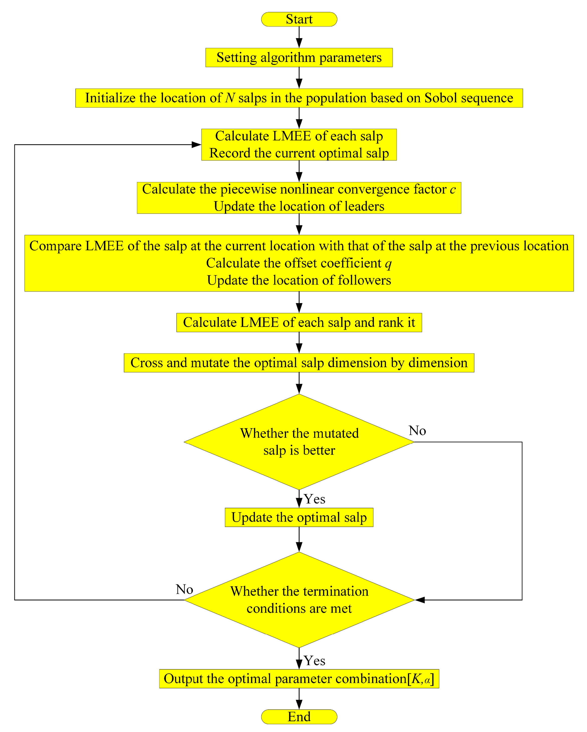
In order to solve the above problems, a rolling bearing fault diagnosis model combining MSSSA-VMD (VMD optimized by the improved salp swarm algorithm based on mixed strategy (MSSSA) [27]) with the parallel network of GASF-CNN (CNN based on Gramian angular summation field (GASF)) and BiLSTM is proposed in this paper. Aiming at the problem that the decomposition effect of VMD is not ideal due to improper parameter selection and the optimal parameter combination [K,α] cannot be obtained by traditional methods, the proposed MSSSA is used to search for the optimal parameter combination [K,α] of VMD; Aiming at the problem that CNN is effective in extracting spatial characteristics but not efficient in extracting temporal characteristics, while BiLSTM excels in temporal characteristic extraction but has limitations in spatial characteristic extraction, CNN and BiLSTM are combined into a parallel network. The advantages of the two are utilized to extract the fault characteristics of rolling bearings fully and comprehensively, Aiming at the problem that one-dimensional signals lack the ability to characterize fault information of rolling bearings and that directly intercepting one-dimensional signals in segments and arranging them in sequence to form two-dimensional signals is easy to cause sample information fragmentation, GASF is utilized to convert one-dimensional signals into two-dimensional signals; In view of the respective advantages and limitations of fault diagnosis methods based on signal processing and deep learning, the two types of methods are integrated. Firstly, the signal processing method (MSSSA-VMD) is employed to preprocess and extract characteristics from the vibration signal of the rolling bearing. Based on the optimal parameter combination, VMD decomposition of the rolling bearing vibration signal is carried out, and the 9 time-domain characteristics (mean, variance, peak value, kurtosis, effective value, peak factor, impulse factor, waveform factor and clearance factor) of the optimal intrinsic mode function (IMF) component of each fault type are extracted to construct characteristic vectors. Secondly, the extracted characteristics are input into the deep learning model (the parallel network of GASF-CNN and BiLSTM) for further analysis and diagnosis. In one channel of the parallel network, GASF is used to convert the characteristic vector extracted by MSSSA-VMD into a two-dimensional image, which is then fed into the CNN for spatial characteristic extraction. In the other channel of the parallel network, the characteristic vector extracted by MSSSA-VMD is directly input into the BiLSTM for temporal characteristic extraction. The extracted spatial and temporal characteristics are fused and then fed into the Softmax classifier for classification.

The contributions of the proposed rolling bearing fault diagnosis model are summarized as follows. Firstly, the proposed MSSSA-VMD can adaptively determine the optimal parameter combination of VMD and then extract the fault characteristics of rolling bearings efficiently. Secondly, the proposed parallel network of GASF-CNN and BiLSTM can make full use of the powerful spatial characteristic extraction capability of CNN and the excellent time series processing performance of BiLSTM, effectively solving the problem of insufficient representation capability of one-dimensional signal for fault information, and use dual-channel parallel training strategy to improve diagnosis efficiency. Thirdly, combining the signal processing method (MSSSA-VMD) with the deep learning method (the parallel network of GASF-CNN and BiLSTM) for rolling bearing fault diagnosis can maximize the advantages of both, thereby effectively enhancing the fault diagnosis performance of the model.

The upcoming sections of this paper are organized as follows: In Section 2, the principles of MSSSA-VMD, CNN, BiLSTM and GASF are explained. A rolling bearing fault diagnosis model combining MSSSA-VMD with the parallel network of GASF-CNN and BiLSTM is proposed in Section 3. In Section 4, experimental verification and result analysis are conducted. Lastly, the conclusions are drawn in Section 5.

2. Basic Theory

2.1. Improved VMD Algorithm

2.1.1. Variational Mode Decomposition

As a completely non-recursive signal processing method, VMD can decompose complex data into simple data with different center frequencies. Each sub-data generated by decomposition is an IMF of the original data, and all the mode functions constitute the original data after superposition. The main principle of VMD is to solve the constrained variational problem.

$$\underset{\left\{u_k\right\},\left\{w_k\right\}}{\min }\left\{{\displaystyle \sum _{k=1}^K{‖g(t)\left[\left(\partial (t)+\frac{j}{\pi t}\right)\ast u_k(t)\right]e^{-j{w}_{k}t}‖}_2^2}\right\}$$

(1)

$$\mathrm{s}.\mathrm{t}. {\displaystyle \sum _{k=1}^K{u}_k}=f(t)$$

(2)

where, u_k is the kth modal component generated by data decomposition, w_k is the center frequency corresponding to the kth modal component, g(t) is the time function, ∂(t) is the impulse function, j is the imaginary unit, t is time, ∗ is the symbol of the convolution operation, and f(t) is the time series.

In order to solve the constrained variational problem, the penalty factor and Lagrange multiplier are introduced, and the constraint condition is transformed into an equality constraint. Thus, the original problem is transformed into an unconstrained variational problem. The converted function is as follows:

$$L(\left\{u_k\right\},\left\{w_k\right\},\lambda )=\alpha {\displaystyle \sum _{k=1}^K{‖g(t)\left[\left(\partial (t)+\frac{j}{\pi t}\right)\ast u_k(t)\right]e^{-j{w}_{k}t}‖}_2^2}+{‖f(t)-u_k(t)‖}_2^2+\left[\lambda (t),f(t)-{\displaystyle \sum _{k=1}^K{u}_k(t)}\right]$$

(3)

where, α is the penalty factor, and λ is the Lagrange multiplier.

The exchange method of multipliers is used to solve the unconstrained variational problem, and the modal component u_k and its center frequency w_k are updated continuously. The expressions for updating u_k and w_k are as follows:

$$u_k^{n+1}(w)={\displaystyle \frac{f(w)-{\displaystyle \sum _{i\ne k}{u}_i(w)+\frac{u(w)}{2}}}{1+2d{(w-w_k)}^2}}$$

(4)

$$w_k^{n+1}={\displaystyle \frac{{\displaystyle {\int }_0^{\infty }w{\left|u_k(w)\right|}^{2}dw}}{{\displaystyle {\int }_0^{\infty }{\left|u_k(w)\right|}^{2}dw}}}$$

(5)

2.1.2. VMD Optimized Based on MSSSA

When using VMD to process the bearing vibration signal, two key parameters of VMD need to be determined, namely, the number of modal components K and penalty factor α. These two parameters restrict each other and jointly determine the signal-processing effect of VMD. If the values of these two parameters are inconsistent, the decomposition effect of VMD will be greatly reduced. However, the values of these two parameters are usually determined empirically, which is highly subjective.

The envelope entropy (EE) can reflect the sparse characteristics of the original signal. The more noise content and less characteristic information contained in the IMF component, the larger the value of EE; Otherwise, the smaller the value of EE.

$$\left\{\begin{array}{l}\mathrm{EE}=-{\displaystyle \sum _{j=1}^M{p}_j}{\log }_2(p_j)\\ p_j={\displaystyle \frac{a(j)}{{\displaystyle \sum _{j=1}^{M}a(j)}}}\end{array}\right.$$

(6)

where, a(j) is the envelope amplitude signal of IMF component obtained after Hilbert demodulation, p(j) is the normalized form of a(j), and M is the length of the IMF component signal.

The envelope entropy is calculated for the K IMF components obtained by decomposition, and the one with the minimum value is referred to as the local minimum envelope entropy (LMEE). Its mathematical expression is shown in Equation (7).

$$\mathrm{LMEE}=\min \left\{\mathrm{EE}(1),\mathrm{EE}(2),\cdots ,\mathrm{EE}(K)\right\}$$

(7)

Therefore, in this paper, LMEE is used as the fitness function, and the improved salp swarm algorithm based on mixed strategy (MSSSA) is used to globally optimize the minimum value of LMEE so as to obtain the optimal parameter combination [K,α] of VMD. MSSSA is a new optimization algorithm proposed by the authors, which has many advantages, such as good global optimization performance, fast convergence, strong robustness and high solving efficiency [27]. The flowchart of optimizing VMD using MSSSA (MSSSA-VMD) is shown in Figure 1.

2.2. Convolutional Neural Network

CNN is a kind of feedforward neural network with convolutional computation and depth structure, which has a strong ability for spatial feature extraction. Compared with fully connected neural networks, CNN greatly reduces the number of parameters and improves the network performance through weight sharing and smooth movement of kernel functions. The basic structure of CNN is shown in Figure 2, which mainly consists of the input layer, convolutional layer, pooling layer, fully connected layer and output layer.

2.3. Bi-Directional Long Short-Term Memory

BiLSTM is an improved form of LSTM, and its network structure is shown in Figure 3. Compared to the traditional LSTM, which only has a unidirectional structure, BiLSTM possesses a bidirectional structure with both forward and backward propagation, and its output is determined by the states of the two oppositely directed LSTM networks. The forward propagation layer trains the time series forward, while the backward propagation layer trains the time series backward. Both the forward propagation layer and the backward propagation layer are connected to the output layer. This structure fully considers the correlation between data nodes in both forward and backward directions and is more suitable for processing time series data with a strong correlation between previous and subsequent moments as well as periodic changes. This significantly improves the characteristic fusion ability of BiLSTM. Therefore, compared with LSTM, characteristics extracted by BiLSTM are more comprehensive.

The operation process of BiLSTM is as follows:

$$\overrightarrow{h_t}=F(w_1{x}_t+w_2{\overrightarrow{h}}_{t-1})$$

(8)

$$\overleftarrow{h_t}=F(w_3{x}_t+w_4{\overleftarrow{h}}_{t+1})$$

(9)

$$O_t=G(w_5\overrightarrow{h_t}+w_6\overleftarrow{h_t})$$

(10)

where, $\overrightarrow{h_t}$ is the output of the forward hidden layer state at time t, $\overleftarrow{h_t}$ is the output of the backward hidden layer state at time t, O_t is the output of the hidden layer state at time t, x_t is the input vector at time t, F is the LSTM unit function, G is the ReLU function, w₁, w₂, w₃, w₄, w₅, and w₆ are weight vectors.

2.4. Visualization of One-Dimensional Time Series Data Based on Gramian Angular Field

Gramian angular field (GAF) can convert one-dimensional time series data into two-dimensional images while maximizing the retention of characteristics from the original signal and avoiding loss of information. Given a time series X = (x₁, x₂, x₃, …, x_m, …, x_s). Where, s is the number of time points, m is a specific time point and m ∈ [1,s]. The specific process of the GAF transformation is described as follows:

Standardization scaling. The time series X in the Cartesian coordinate system is normalized and compressed to $\stackrel{<}{x}$_m within the range of [−1, 1] using Equation (11).

$${\stackrel{<}{x}}_m={\displaystyle \frac{x_m-\max (X)+x_m-\min (X)}{\max (X)-\min (X)}}$$

(11)

where, $\stackrel{<}{x}$_m ∈ [−1, 1].

Conversion of polar coordinates. The definition of a Gram matrix is shown in Equation (12).

$$G=X^{T}X=\left[\begin{array}{l}<x_1,x_1>\cdots <x_1,x_s>\\ <x_2,x_1>\cdots <x_2,x_s>\\ ⋮\\ <x_s,x_1>\cdots <x_s,x_s>\end{array}\right]$$

(12)

where, G is the Gram matrix, and <·> is the inner product operation.

The vibration data of the rolling bearing are converted to vectors by polar coordinates. The transformation formula is shown in Equation (13).

$$\left\{\begin{array}{l}\varphi =\arccos ({\stackrel{<}{x}}_m), -1\le {\stackrel{<}{x}}_m\le 1,{\stackrel{<}{x}}_m\in \stackrel{<}{X}\\ R={\displaystyle \frac{t_i}{N}},t_i=1,2,\cdots ,N\end{array}\right.$$

(13)

where, t_i is the timestamp, N is the constant factor for normalizing the polar coordinate generation space, ϕ is the phase angle, R is the polar coordinate radius, and $\stackrel{<}{X}$ is the normalized and compressed X.

Gramian angular field. GAF defines two unique inner product forms with penalty terms to eliminate the impact of Gaussian noise. Their definitions are as follows:

$$<x_m,x_n>=\cos ({\varphi }_m+{\varphi }_n)$$

(14)

$$<x_m,x_n>=\sin ({\varphi }_m-{\varphi }_n)$$

(15)

For the above two different definitions of inner product, two different GAFs can be obtained: Gramian angular summation field (GASF) and Gramian angular difference field (GADF). In this paper, GASF is used to convert rolling bearing vibration data into two-dimensional images.

3. A Rolling Bearing Fault Diagnosis Model Combining MSSSA-VMD with the Parallel Network of GASF-CNN and BiLSTM

A rolling bearing fault diagnosis model combining MSSSA-VMD with the parallel network of GASF-CNN and BiLSTM is proposed in this paper. The overall structure and fault diagnosis process of the proposed model are shown in Figure 4.

The proposed model consists of two parts:

Part 1: Preprocessing and characteristic extraction based on MSSSA-VMD. According to the process shown in Figure 1, MSSSA is used to optimize VMD to obtain the optimal parameter combination of VMD. Based on the optimal parameter combination, VMD decomposition is performed on the rolling bearing vibration signal, and then the 9 time-domain characteristics (mean, variance, peak value, kurtosis, effective value, peak factor, impulse factor, waveform factor and clearance factor) of the optimal IMF component of each fault type are extracted to construct vectors.

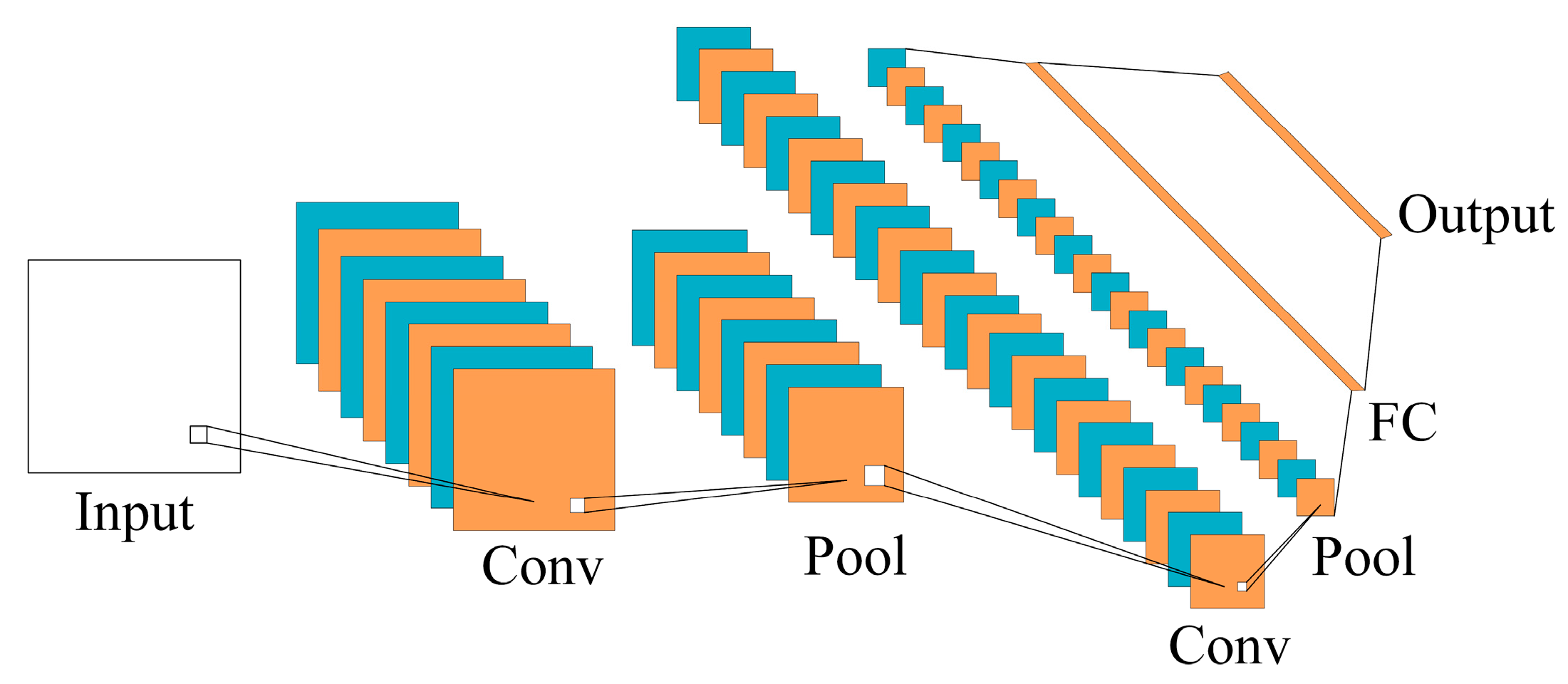
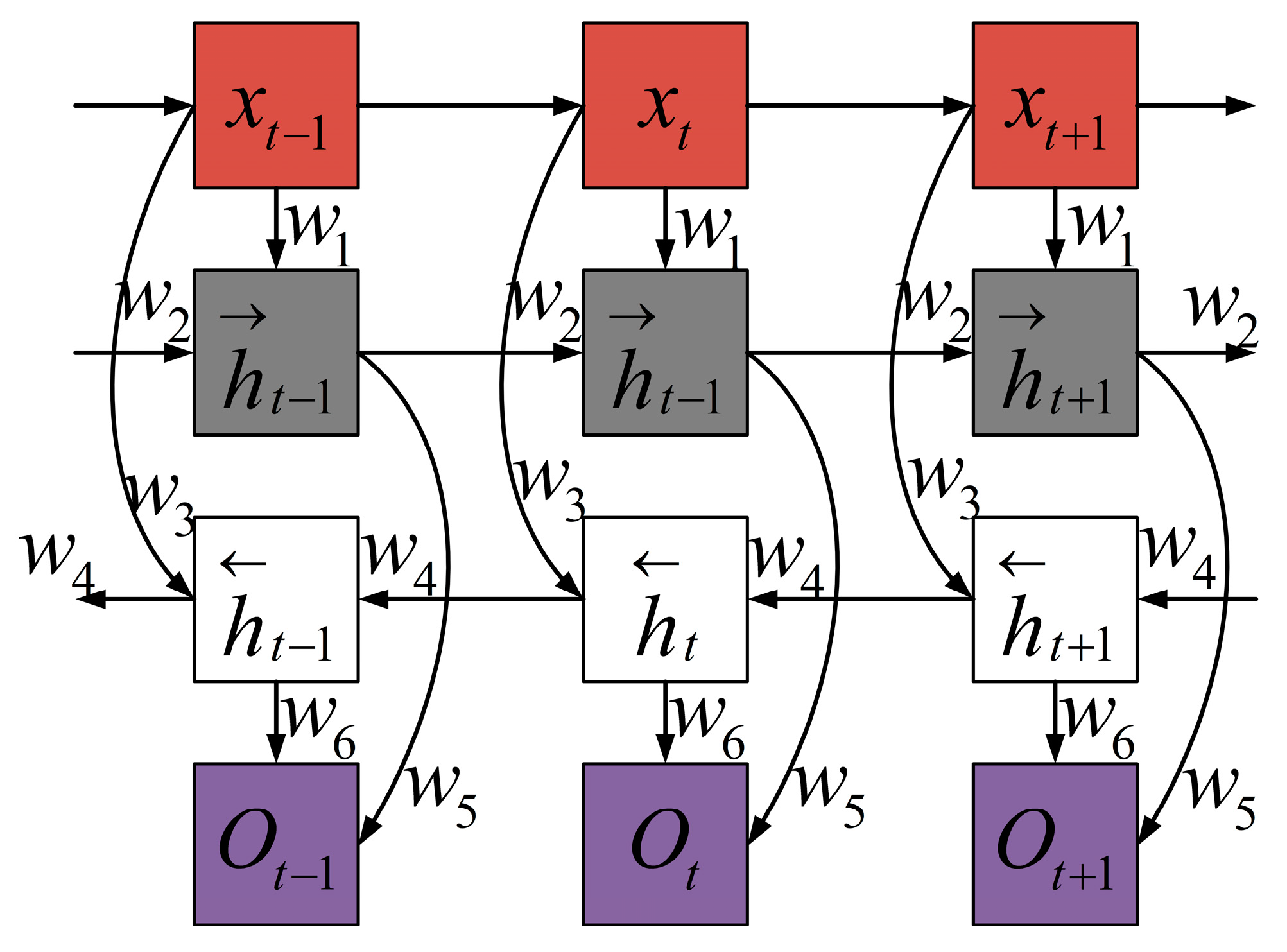
Part 2: Fault diagnosis based on the parallel network of GASF-CNN and BiLSTM. In one channel, the characteristic vectors are converted into a two-dimensional image by GASF and fed into CNN. Then, the spatial characteristics of the two-dimensional image are extracted by CNN through convolution and pooling, and a set of one-dimensional vectors is outputted through the fully connected layer. In the other channel, the characteristic vectors are directly fed into BiLSTM, where their temporal characteristics are extracted. Then, a set of one-dimensional vectors is outputted through the fully connected layer. Afterward, the two sets of one-dimensional vectors are fused. Finally, the fused characteristics are sent to the Softmax classifier for classification.

4. Experimental Verification and Result Analysis

4.1. Experimental Verification and Result Analysis Based on CWRU Bearing Dataset

4.1.1. Description and Preprocessing of Experimental Data (CWRU Bearing Dataset)

The most objective way to evaluate the performance of the proposed model is to compare it with existing models using a third-party standard database. The rolling bearing dataset used in this experiment comes from the bearing data center of Case Western Reserve University (CWRU) [28], which is a globally recognized standard dataset for bearing fault diagnosis. The experimental platform of CWRU bearing dataset is shown in Figure 5. Artificial single-point failures with different pitting diameters were created using electrical discharge machining technology. Acceleration transducers were used to collect vibration acceleration signals, while the torque transducer was employed to collect data on speed and power. The drive-end bearing with model number SKF6205 was selected, and the sampling frequency of the system was set at 12 kHz. Based on different motor rotation speeds (1797 r/min, 1772 r/min, 1750 r/min, and 1730 r/min), data were collected under four load conditions (0 HP, 1 HP, 2 HP, and 3 HP). The fault diameters of the bearing are classified into three categories: 0.1778 mm, 0.3556 mm, and 0.5334 mm, representing different levels of fault severity. There are a total of 10 types of bearing faults, including inner raceway faults (with three different fault diameters), outer raceway faults (with three fault diameters), rolling element faults (with three different fault diameters), and the normal condition.

The deep learning model requires a large number of samples for training. If the number of training samples is insufficient, overfitting will occur, which will lead to poor performance of the model. However, in the actual operation process, the rolling bearing cannot maintain the working state for a long time after the fault occurs, so it is difficult to obtain enough fault samples for training. Therefore, it is necessary to use data augmentation technology to increase the number of training samples required by the training model to meet the demand for experimental data. Data augmentation is a technique that can effectively solve the problem of data imbalance. Applying specific rules to increase the number of samples can effectively reduce the risk of overfitting and consequently enhance the generalization ability of the model.

Overlapping sampling is a data augmentation method that not only effectively expands the number of training samples but also fully retains the temporality and periodicity of one-dimensional sequences. Therefore, the overlapping sampling method is used to augment the data of this experiment. The core idea of the overlapping sampling method is as follows: Sliding sampling is carried out according to a certain step size to create an overlapping area between adjacent samples so as to increase the number of samples and effectively solve the problem of sample edge information loss. The process of overlapping sampling is shown in Figure 6, and its calculation formula is expressed in Equation (16).

$$X={\displaystyle \frac{l-Q}{S}}+1, l>>Q$$

(16)

where, l is the length of the input original data, Q is the length of the sliding window, S is the step size, and X is the number of samples after overlapping sampling processing.

When performing overlapping sampling, the step size is set to 1000, and the length of the sliding window is set to 2048 data points to ensure the integrity and validity of the bearing fault information contained in the experimental data. The original data is segmented to obtain 120 samples for each fault type, totaling 1200 samples. The data size of each sample is 1 × 2048. The labeled dataset corresponding to the 10 fault types is shown in

Table 1. The labeled dataset corresponds to the 10 fault types.

Operating Condition	Fault Type	Fault Diameter/mm	The Number of Samples	Fault Label
0 HP/1 HP/2 HP/3 HP	Normal	—	120	0
	IF07	0.1778	120	1
	BF07	0.1778	120	2
	OF07	0.1778	120	3
	IF014	0.3556	120	4
	BF014	0.3556	120	5
	OF014	0.3556	120	6
	IF021	0.5334	120	7
	BF021	0.5334	120	8
	OF021	0.5334	120	9

. MSSSA-VMD is used to process the rolling bearing vibration data of 10 fault types to obtain the optimal IMF component corresponding to each fault type. Then 9 time-domain characteristics (mean, variance, peak value, kurtosis, effective value, peak factor, impulse factor, wave-form factor and clearance factor) of the optimal IMF component corresponding to each fault type are extracted to form a characteristic dataset.

4.1.2. Presentation of Training Results

The proposed model is built based on the software MATLAB R2023a, and the hardware it relies on includes an Intel(R) Core(TM) i5-14600KF CPU originates from Santa Clara, CA, United States, an NVIDIA RTX 4060Ti GPU originates from Santa Clara, CA, United States, and 32 GB of RAM. The training parameters of the model are set as follows: The max epoch is set to 150, the initial learning rate is set to 0.001, the learning rate drop period is set to 100, and the learning rate drop factor is set to 0.01. The Adam optimizer is used for optimization, and the cross entropy loss function is selected as the loss function. The ReLU function is selected as the activation function, and the maximum pooling is selected as the pooling type. The 2D convolutional layer has a kernel size of 5 × 5, a stride of [1, 1], and a number of kernels equal to 10. The pooling layer has a kernel size of 2 × 2, a stride of [2, 2], and a number of kernels equal to 10.

The obtained characteristic dataset is randomly divided into a training set and a test set according to the ratio of 7:3. The training set is fed into the parallel network of GASF-CNN and BiLSTM for training: The GASF image obtained by transforming the characteristic data is fed into CNN, while the characteristic data itself is fed into BiLSTM.

In order to verify the ability of fault characteristic extraction and classification of the proposed model, the t-distributed stochastic neighbor embedding (t-SNE) algorithm was utilized to visualize the rolling bearing fault classification process based on the proposed model. The characteristic distributions of the original signal, CNN layer, BiLSTM layer, and Softmax layer are shown in Figure 7 (limited by space, only 0 HP operating condition is taken as an example).

The characteristic distribution of the original signal is completely disorganized, exhibiting the highest degree of confusion. In the CNN layer and BiLSTM layer, fault characteristics of the same type begin to cluster together, gradually forming their own communities, and the boundaries between different types of fault characteristics gradually become clearer. However, there are still noticeable overlaps in the distribution of fault characteristics of different types, making it difficult to distinguish them. In the Softmax layer, fault characteristics of the same type are highly compact and have formed individual, isolated communities, and fault characteristics of different types have been almost completely distinguished from each other. Compared to using a single CNN channel or a single BiLSTM channel, the clustering effect obtained by fusing the two parallel channels of CNN and BiLSTM is significantly improved, and the degree of confusion between different fault characteristics is also greatly reduced. This validates the superiority of the parallel dual-channel fusion strategy employed by the proposed model. In summary, the proposed model can effectively identify the fault types of rolling bearings and its capability for fault characteristic extraction and classification has been proved.

4.1.3. Comparison with Baseline Models

To verify the performance of the proposed model (Model A), it was compared with several baseline models. The baseline models are shown in

Table 2. Baseline models are used to compare the proposed model.

Model	Name
MSSSA-VMD + parallel CNN based on GAF + BiLSTM	B
MSSSA-VMD + parallel CNN based on GAF + GRU	C
MSSSA-VMD + parallel CNN based on GAF + LSTM	D
MSSSA-VMD + parallel CNN based on GAF	E
MSSSA-VMD + GADF-CNN + BiLSTM	F
MSSSA-VMD + GADF-CNN + GRU	G
MSSSA-VMD + GADF-CNN + LSTM	H
MSSSA-VMD + GADF-CNN	I
MSSSA-VMD + GASF-CNN + BiLSTM	J
MSSSA-VMD + GASF-CNN + GRU	K
MSSSA-VMD + GASF-CNN + LSTM	L
MSSSA-VMD + GASF-CNN	M
Parallel network of GASF-CNN and BiLSTM	N
Parallel CNN based on GAF + BiLSTM	O
Parallel CNN based on GAF + GRU	P
Parallel CNN based on GAF + LSTM	Q
Parallel CNN based on GAF	R
CNN + BiLSTM	S
CNN + GRU	T
CNN + LSTM	U
CNN	V

.

Verification of Fault Diagnosis Performance Under Constant Operating Conditions

The average of the five experimental results was taken as the final experimental result, and the diagnostic accuracy of each model under constant operating conditions was obtained, as shown in

Table 3. The diagnostic accuracy of each model under constant operating conditions (comparison with baseline models).

Model	Accuracy/%
	0 HP	1 HP	2 HP	3 HP	Average
A	99.33	99.22	98.95	98.72	99.06
B	98.28	97.44	97.16	96.67	97.39
C	98.00	97.17	96.78	95.34	96.82
D	97.72	96.89	96.45	95.22	96.57
E	97.16	96.28	95.78	94.11	95.83
F	97.44	96.50	96.05	94.65	96.16
G	96.89	96.33	95.22	94.39	95.71
H	96.61	96.05	95.06	94.11	95.46
I	96.05	95.50	94.39	93.83	94.94
J	97.16	96.05	95.50	94.11	95.71
K	96.61	95.78	94.89	93.83	95.28
L	96.45	95.50	94.78	93.55	95.07
M	95.50	94.39	94.06	93.28	94.31
N	97.28	96.50	95.34	94.50	95.91
O	96.72	96.05	94.94	94.22	95.48
P	96.45	95.78	94.66	93.95	95.21
Q	96.17	95.89	94.39	93.83	95.07
R	95.61	95.22	94.22	93.28	94.58
S	95.89	95.45	94.55	93.00	94.72
T	95.50	94.94	94.39	92.84	94.42
U	95.34	94.94	94.22	92.83	94.33
V	94.78	94.06	93.50	92.33	93.67

. The fault diagnosis performance of each model is different under different operating conditions, and the diagnostic accuracy of low-load conditions is generally higher than that of high-load conditions. Through comparison, it can be found that the overall performance of the proposed model (Model A) is the best, and its diagnostic accuracy is higher than that of other models under all operating conditions. The diagnostic accuracy is as high as 99.33% under 0 HP operating conditions, and the diagnostic accuracy can still maintain 98.72% even if the performance is reduced under 3 HP operating conditions. Its average diagnostic accuracy is as high as 99.06%. This is mainly due to the following advantages: Using MSSSA-VMD for preprocessing and characteristic extraction can separate the noise component in the signal from the fault characteristic component to improve the signal quality and then obtain characteristics with clearer fault mode, which helps the deep learning model to identify fault types more accurately; The deep learning model adopts the parallel network of GASF-CNN and BiLSTM. The combination of CNN and BiLSTM can fully extract the spatial characteristics and temporal characteristics to obtain more comprehensive information on rolling bearing fault characteristics. The two-dimensional time-frequency image obtained by GASF transformation can effectively capture the time-frequency characteristics of the signal at different scales. The dual-channel parallel strategy can achieve characteristic fusion and improve the robustness of the model. The diagnostic accuracy of the eight models, F, G, H, I, J, K, L and M, is lower than that of the four models, B, C, D and E, mainly because, compared with the two-channel parallel network, the robustness and flexibility of the single-channel network are poor, leading to its inadequate adaptability to complex fault modes. As for CNN (Model V), due to the lack of ability to extract time series characteristics, it is unable to extract fault characteristics of time series data, such as rolling bearing vibration data adequately, coupled with insufficient data preprocessing, resulting in the worst fault diagnosis performance. Its average diagnostic accuracy is only 93.67%, which is 5.39% lower than the proposed model. It can be seen from the above analysis that the proposed model has good fault diagnosis performance under different operating conditions.

Verification of Generalization Ability Under Variable Operating Conditions

The composition of the experimental dataset under variable operating conditions is shown in

Table 4. The composition of the experimental dataset under variable operating conditions.

Dataset	Change of Operating Condition
a→b	0 HP→1 HP
a→c	0 HP→2 HP
a→d	0 HP→3 HP
b→a	1 HP→0 HP
b→c	1 HP→2 HP
b→d	1 HP→3 HP
c→a	2 HP→0 HP
c→b	2 HP→1 HP
c→d	2 HP→3 HP
d→a	3 HP→0 HP
d→b	3 HP→1 HP
d→c	3 HP→2 HP

. The average of five experimental results was taken as the final experimental result, and the diagnostic accuracy of each model under variable operating conditions was obtained, as shown in

Table 5. The diagnostic accuracy of each model under variable operating conditions (comparison with baseline models).

Model	Accuracy/%
	a→b	a→c	a→d	b→a	b→c	b→d	c→a	c→b	c→d	d→a	d→b	d→c	Average
A	98.50	94.76	94.44	97.89	90.50	96.06	85.94	94.22	96.72	88.06	95.50	97.33	94.16
B	97.37	92.22	90.39	95.89	84.11	94.83	86.17	92.67	94.39	89.28	94.78	95.50	92.30
C	97.28	96.05	92.05	94.00	88.45	92.67	87.00	88.61	92.83	81.01	92.39	94.94	91.44
D	97.22	93.00	86.00	95.06	90.00	94.06	83.06	87.22	94.78	85.17	92.16	94.11	90.99
E	97.01	90.00	89.22	94.89	81.94	92.16	84.22	87.78	94.06	87.00	92.93	93.94	90.43
F	96.95	89.50	88.00	95.06	91.16	94.00	84.28	82.06	92.22	84.89	93.17	94.05	90.45
G	96.72	89.94	87.44	96.11	87.94	95.00	81.33	86.00	94.11	79.34	92.33	93.00	89.94
H	96.11	88.89	87.84	95.56	87.28	94.11	83.17	83.94	92.05	81.89	89.50	93.39	89.48
I	95.43	86.28	85.00	95.00	89.00	92.22	79.39	81.89	93.00	83.89	89.83	93.51	88.70
J	96.83	89.78	87.83	95.55	84.39	94.06	76.11	87.33	94.00	81.89	92.44	93.89	89.51
K	96.39	92.16	84.05	95.11	87.22	91.72	77.61	86.06	94.11	78.39	91.05	93.11	88.92
L	96.05	88.61	82.84	95.06	87.11	91.11	77.39	85.22	94.10	81.78	90.83	92.06	88.51
M	94.83	87.94	86.67	94.11	85.22	92.16	76.84	84.55	93.06	78.39	89.00	93.06	87.99
N	96.28	90.56	86.28	95.39	89.44	93.06	81.06	87.95	94.06	85.00	92.18	94.00	90.44
O	96.44	88.56	87.33	95.55	85.61	92.95	79.55	89.06	93.94	82.06	91.44	92.36	89.57
P	95.89	90.28	86.23	94.06	87.50	93.56	77.50	86.06	91.44	80.01	92.11	93.06	88.98
Q	95.44	87.61	87.00	94.06	86.28	92.00	78.00	85.39	93.50	78.78	91.61	93.00	88.56
R	95.28	87.94	85.22	95.05	86.00	90.89	76.95	85.06	92.94	79.39	88.94	93.06	88.06
S	95.05	87.06	85.00	94.94	84.17	89.94	74.17	83.56	93.50	77.96	88.00	92.00	87.11
T	94.50	86.50	85.61	94.60	81.12	89.72	73.45	84.44	91.39	77.57	87.39	91.61	86.49
U	94.56	86.06	81.12	94.06	83.89	88.94	71.66	82.91	92.16	76.96	87.17	92.50	86.00
V	93.90	84.83	84.00	93.06	80.00	88.00	71.32	82.89	89.94	75.94	86.00	92.16	85.17

.

For example, 0 HP→1 HP, when the operating conditions of the training set and the test set are similar, the diagnostic accuracy of each model is generally higher. However, for example, 0 HP→3 HP, when the operating conditions of the training set and the test set are different, the diagnostic accuracy of each model is significantly reduced. Among all models, the proposed model (Model A) has the highest diagnostic accuracy under variable operating conditions, with an average diagnostic accuracy of 94.16%. Under the operating condition of 0 HP→1 HP, when the training set and the test set are close to each other, the diagnostic accuracy is as high as 98.50%, which is higher than other models. Under the operating conditions of the big difference between the training set and test set, such as 2 HP→0 HP, its diagnostic accuracy drops to 85.94%, but it is still higher than that of other models. The above results are mainly benefited from: Using MSSSA-VMD for preprocessing and characteristic extraction can remove the unfavorable factors contained in the original data, such as irrelevant features, missing values, outliers and redundant information to improve data quality, thus laying a good foundation for subsequent model training; The deep learning model adopts the parallel network of GASF-CNN and BiLSTM, which can effectively capture subtle changes in the complex signal under variable operating conditions and fully mine fault characteristic information, thus greatly enhancing the model’s adaptability to unknown operating conditions. CNN (Model V) has the worst fault diagnosis performance under variable operating conditions, and its average diagnosis accuracy is only 85.17%, which is 8.99% lower than that of the proposed model. This is mainly because there is no effective preprocessing of the data, which leads to the inability to balance the characteristic distribution, and it is difficult to capture the long-term dependence relationship in the time series data, which leads to the inability to effectively extract the fault characteristics under variable operating conditions, resulting in poor generalization ability. The diagnostic accuracy of the four models B, C, D and E is higher than that of the four models O, P, Q and R under variable operating conditions, which proves the effectiveness of using MSSSA-VMD for preprocessing and characteristic extraction to enhance the generalization ability of the model. According to the above analysis, compared with the constant operating conditions, the fault diagnosis accuracy of each model under variable operating conditions decreases to varying degrees, but the proposed model can still maintain a high diagnostic accuracy, which indicates that the proposed model has good generalization ability and can effectively deal with the requirement of rolling bearing fault diagnosis under variable operating conditions.

Verification of Noise Resistance

The noise resistance determines the fault diagnosis performance of the model to some extent, so it is necessary to verify the noise resistance of the model. White Gaussian noise with different intensities is added to the experimental dataset to simulate the noise interference of rolling bearings in the actual working environment. The average of the five experimental results was taken as the final experimental result, and the diagnostic accuracy of each model under different noise intensities was obtained, as shown in Figure 8 (limited by space, only 0 HP operating condition was taken as an example).

It can be seen that all models have good fault diagnosis performance under a weak noise environment. When SNR is 8 dB, the diagnostic accuracy of all models is above 90.00%, among which, the proposed model (Model A) has the highest diagnostic accuracy (98.67%), and CNN (Model V) has the lowest diagnostic accuracy (92.61%). With the continuous increase of noise, the fault diagnosis accuracy of each model decreases to different degrees. Among them, CNN has the largest decline, and its diagnosis accuracy drops to 42.24% under −4 dB noise intensity, while the proposed model has the smallest decline, and its diagnosis accuracy is still higher than other models under −4 dB noise intensity. The reasons for the above results are as follows: All time points in the vibration signal of rolling bearings are correlated, and CNN cannot capture the long-term dependence in the signal, resulting in the loss of time sequence information. As a result, CNN cannot effectively extract fault characteristic information of rolling bearings in a strong noise environment. The proposed model integrates the spatial characteristics extracted by CNN with the temporal characteristics extracted by BiLSTM so that it can mine the fault characteristic information of rolling bearings to the maximum extent under a strong noise environment so as to obtain good noise resistance. Through comparison, it can be found that the diagnostic accuracy of model N under different noise intensities is significantly lower than that of the proposed model, which proves that using MSSSA-VMD for preprocessing and characteristic extraction can effectively improve the noise resistance of the model. In addition, the fault diagnosis performance of the four models B, C, D and E is better than that of the eight models F, G, H, I, J, K, L and M under noise interference, which proves that the dual-channel parallel training strategy can effectively improve the noise resistance of the model. In summary, the proposed model has good noise resistance and can effectively diagnose rolling bearing faults under noise interference.

Evaluation of Computation Time

The calculation time is also an important index to evaluate the performance of the model. The calculation time and diagnostic accuracy of each model under 0 HP operating conditions are shown in

Table 6. The calculation time and diagnostic accuracy of each model (0 HP).

Model	Accuracy	Computation Time/s
A	99.33	101.16
B	98.28	189.21
C	98.00	190.52
D	97.72	188.96
E	97.16	187.05
F	97.44	160.22
G	96.89	154.17
H	96.61	151.71
I	96.05	146.82
J	97.16	159.86
K	96.61	153.95
L	96.45	151.62
M	95.50	146.34
N	97.28	105.67
O	96.72	189.40
P	96.45	191.05
Q	96.17	189.32
R	95.61	188.39
S	95.89	96.91
T	95.50	96.57
U	95.34	95.86
V	94.78	92.25

(the average of the five experimental results is taken as the final experimental result).

As can be seen from Table 6, the inference time of the proposed model is shorter than that of most models, only slightly longer than that of the four models S, T, U and V, but its diagnostic accuracy is significantly higher than that of the four models S, T, U and V. MSSSA-VMD can greatly reduce the dimension of data and effectively eliminate redundant information in the data. Meanwhile, the IMF components obtained by MSSSA-VMD decomposition can reflect the characteristic information and structure information of the signal well, thus improving the effectiveness of characteristic extraction. Therefore, the inference speed of the proposed model can be greatly improved. In addition, the dual-channel parallel training strategy adopted by the parallel network of GASF-CNN and BiLSTM also effectively reduces the inference time of the proposed model. In summary, it can be seen that the proposed model sacrifices a certain amount of inference time to obtain higher diagnostic accuracy, stronger generalization ability and better noise resistance. The proposed model exhibits high diagnostic efficiency for rolling bearing faults and can meet real-time requirements in practical engineering applications.

4.1.4. Comparison with Classical Fault Diagnosis Models (CWRU Bearing Dataset)

In order to further verify the performance of the proposed model, it is compared with three classical fault diagnosis models, namely support vector machine (SVM), LeNet-5 and wide deep convolutional neural networks (WDCNN).

Verification of Fault Diagnosis Performance Under Constant Operating Conditions

The rolling bearing fault diagnosis experiment under constant operating conditions was carried out, and the average of the five experimental results was taken as the final experimental result. The diagnostic accuracy of the four models under constant operating conditions is shown in

Table 7. The diagnostic accuracy of each model under constant operating conditions (comparison with classical fault diagnosis models).

Model	Accuracy/%
	0 HP	1 HP	2 HP	3 HP	Average
SVM	89.06	88.43	87.36	86.81	87.92
LeNet-5	95.19	94.56	93.97	92.52	94.06
WDCNN	96.26	96.24	96.07	95.82	96.10
Proposed model	99.33	99.22	98.95	98.72	99.06

and Figure 9.

SVM, as a traditional machine learning model, has the lowest diagnostic accuracy and is significantly lower than the other three models with convolutional structures. This is because SVM has insufficient characteristic extraction capability for high-dimensional data, resulting in its inability to effectively extract high-level characteristics in the data. Compared with SVM, the diagnostic accuracy of LeNet-5 and WDCNN is greatly improved, which indicates that the convolutional structure has a more powerful characteristic extraction ability and can extract more abstract characteristics. However, the diagnostic effect of the two is still not ideal. This is because the convolutional structure lacks the ability to extract time series characteristics, resulting in inadequate characteristic extraction of time series data, such as rolling bearing vibration data, which restricts its fault diagnosis performance. The diagnostic accuracy of the proposed model is the highest, which is significantly higher than that of the other three models under all operating conditions, and its average diagnostic accuracy is 11.14%, 5.00% and 2.96% higher than that of SVM, LeNet-5 and WDCNN, respectively, indicating that multiple strategies adopted by the proposed model are reasonable and effective: MSSSA-VMD is used to pre-process the original vibration signal and extract characteristics, which can effectively remove redundant characteristics, further enhance the characteristic extraction capability of the deep learning model, and greatly reduce the computational complexity; The deep learning model adopts the parallel network of GASF-CNN and BiLSTM, which can maximize the powerful spatial characteristic extraction capability of CNN and the excellent time series processing performance of BiLSTM, and effectively solve the problem of insufficient representation ability of one-dimensional signal for rolling bearing fault information. In summary, the proposed model can effectively extract the fault characteristics of rolling bearings and has good fault diagnosis performance under different operating conditions.

Verification of Generalization Ability Under Variable Operating Conditions

The average of the five experimental results was taken as the final experimental result, and the diagnostic accuracy of the four models under variable operating conditions was obtained, as shown in Figure 10.

SVM has the lowest fault diagnosis accuracy under variable operating conditions and is significantly lower than the other three models (its average diagnosis accuracy is only 69.27%). This is because its generalization ability is largely affected by the kernel function and penalty factor. If the kernel function does not match the characteristics of the dataset, the model will not be able to effectively capture the change of data distribution brought about by the change of operating conditions, while if the penalty factor is improperly selected, the model will be overfitted, both of which will lead to the decline of its generalization ability. The average diagnostic accuracy of LeNet-5 is 85.44%. Compared with SVM, the fault diagnosis performance under variable operating conditions of LeNet-5 has been greatly improved, but it is still not good. This is because its convolutional structure is relatively simple. In the face of complex and changeable operating conditions, the model may not be able to fully capture the characteristic information in the data due to insufficient capacity, resulting in poor generalization ability. The average diagnostic accuracy of WDCNN is 90.30%, and its fault diagnosis performance under variable operating conditions is better than SVM and LeNet-5, but it is still not ideal. This is because it is unable to effectively preprocess the noise and outliers contained in the variable operating condition data and fails to select the representative characteristics sensitive to the change of operating condition, resulting in its unsatisfactory generalization ability. The proposed model has the highest fault diagnosis accuracy under variable operating conditions, and its average diagnosis accuracy is 24.89%, 8.72% and 3.86% higher than SVM, LeNet-5 and WDCNN, respectively, mainly due to: Using MSSSA-VMD for preprocessing and characteristic extraction can effectively eliminate noise and outliers in the data and balance the data distribution, which helps the model to better identify key characteristics under variable operating conditions; The deep learning model adopts the parallel network of GASF-CNN and BiLSTM, which can effectively extract and fuse characteristics, thus helping the model to learn more abundant characteristic information and accurately capture the subtle changes in the vibration signal of the rolling bearing, so as to better understand the complex change patterns and rules of data under variable operating conditions. In conclusion, the proposed model has good generalization ability and can effectively deal with the requirement of rolling bearing fault diagnosis under variable operating conditions.

Verification of Noise Resistance

The average of the five experimental results was taken as the final experimental result, and the diagnostic accuracy of the four models under different noise intensities was obtained, as shown in Figure 11 (Only 0 HP operating condition was taken as an example).

As can be seen from Figure 11, the fault diagnosis performance of each model decreases to varying degrees with the increasing noise intensity. Among them, SVM has the worst noise resistance, and its diagnostic accuracy decreases the most with noise enhancement, from 86.92% when SNR is 8 dB to 41.05% when SNR is −4 dB. This is because its fault diagnosis performance is largely affected by characteristic selection. Improper characteristic selection results in the lowest diagnostic accuracy and the most drastic change under different noise intensities, which indicates that the nonlinear characteristics of the rolling bearing vibration signal cannot be effectively extracted. The diagnostic accuracy of LeNet-5 is higher than that of SVM under different noise intensities, and its diagnostic accuracy decreases slightly with the increase of noise, from 93.32% when SNR is 8 dB to 57.12% when SNR is −4 dB. This is because its convolutional structure can extract relatively abstract characteristics, thereby reducing the impact of noise interference on its fault diagnosis performance to a certain extent. However, due to its relatively simple convolutional structure, it cannot fully extract weak fault characteristic information in a strong noise environment, so its fault diagnosis performance under strong noise interference is poor. The diagnostic accuracy of WDCNN under 8 dB noise intensity and −4 dB noise intensity is 94.91% and 74.72%, respectively. The noise resistance of WDCNN is better than that of SVM and WDCNN, and it can maintain relatively good fault diagnosis performance under noise interference. This is because the wide convolution kernel structure adopted in the first layer further strengthens its characteristic extraction capability and thus enhances its noise robustness to a certain extent. However, when dealing with the complex and variable vibration signals of rolling bearings under strong noise interference, it still has the problem of inadequate characteristic extraction, and the convolution kernel is not optimized for noise, so it cannot effectively distinguish the fault characteristics of rolling bearings from the noise characteristics, resulting in its fault diagnosis performance under noise interference is still not ideal. The noise resistance of the proposed model is significantly better than that of the other three models. The fault diagnosis accuracy of the proposed model is the highest under different noise intensifications. Even under the strong noise interference of −2 dB, it can still maintain an accuracy of more than 90.00%, and the diagnostic accuracy decreases minimally with the increase of noise. This is mainly due to the fact that using MSSSA-VMD for data preprocessing and characteristic extraction can effectively remove noisy data and enhance the characteristic extraction capability of the model. The parallel network of GASF-CNN and BiLSTM can further strengthen the model’s ability to capture weak fault characteristic information under noise interference, thus greatly enhancing the robustness of the model. The results show that the proposed model has reliable noise resistance and can effectively deal with the requirement of rolling bearing fault diagnosis under different noise intensities.

4.2. Experimental Verification and Result Analysis Based on JNU Bearing Dataset

4.2.1. Description and Preprocessing of Experimental Data

In order to ensure the rigor and practicability of the research, the bearing dataset provided by Jiangnan University (JNU) is used to further verify the performance of the proposed model [29]. The JNU bearing dataset is derived from a real experimental environment and aims to provide standardized data for the evaluation of bearing performance. The experimental platform of the JNU bearing dataset is the centrifugal fan rolling bearing fault acquisition device, as shown in Figure 12. The motor used is a three-phase induction motor; the rated power is 3.7 kW, and the rated speed is 1800 r/min. The accelerometer used is the PCBMA352A60 accelerometer, which is manufactured in the United States. The test bearings are N205 bearing and NU205 bearing, both produced by LYCRH, located in Luoyang, China. The vibration signal in the vertical direction of the test bearing was collected at a sampling frequency of 50 kHz and a collection time of 20 s. The experiment covers three different operating conditions (600 r/min, 800 r/min and 1000 r/min); each operating condition contains four bearing fault types: normal, inner race fault, outer race fault and ball fault.

When performing overlapping sampling, the step size is set to 1000, and the length of the sliding window is set to 2048 data points. The original data is segmented to obtain 120 samples for each fault type, totaling 480 samples. The data size of each sample is 1 × 2048. The labeled dataset corresponding to the four fault types is shown in

Table 8. The labeled dataset corresponds to the four fault types.

Operating Condition	Fault Type	The Number of Samples	Fault Label
600 r/min	Normal	120	1
	Inner race fault	120	2
	Outer race fault	120	3
	Ball fault	120	4
800 r/min	Normal	120	1
	Inner race fault	120	2
	Outer race fault	120	3
	Ball fault	120	4
1000 r/min	Normal	120	1
	Inner race fault	120	2
	Outer race fault	120	3
	Ball fault	120	4

. MSSSA-VMD is used to process the rolling bearing vibration data of 4 fault types to obtain the optimal IMF component corresponding to each fault type. Then, nine time-domain characteristics of the optimal IMF component corresponding to each fault type are extracted to form a characteristic dataset.

4.2.2. Comparison with Classical Fault Diagnosis Models

The proposed model is compared with three classic fault diagnosis models, namely SVM, LeNet-5, and WDCNN, to further verify its performance.

Verification of Fault Diagnosis Performance Under Constant Operating Conditions

The average of the five experimental results was taken as the final experimental result, and the diagnostic accuracy of the four models under constant operating conditions was obtained, as shown in

Table 9. The diagnostic accuracy of each model under constant operating conditions.

Model	Accuracy/%
	600 r/min	800 r/min	1000 r/min	Average
SVM	80.66	84.13	86.52	83.77
LeNet-5	86.71	91.22	92.41	90.11
WDCNN	90.82	93.05	94.27	92.71
Proposed model	95.98	96.91	97.20	96.70

and Figure 13.

The diagnostic accuracy of the traditional machine learning model SVM under different operating conditions is significantly lower than that of the other three deep learning models, and its average diagnostic accuracy is only 83.77%. Compared with deep learning models, its processing ability for high-dimensional complex data is relatively insufficient, and its capturing ability for data distribution and inherent laws is relatively weak, resulting in its inability to effectively extract fault characteristics in complex fault diagnosis tasks. The fault diagnosis performance of LeNet-5 and WDCNN under constant operating conditions is better than that of SVM. The average diagnostic accuracy of LeNet-5 and WDCNN is 90.11% and 92.71%, respectively. Compared with SVM, the performance is highly dependent on characteristic selection, LeNet-5 and WDCNN can automatically extract more abstract and deep characteristics from the original data through the convolution structure, and the model learned through a large number of training data has a relatively better generalization ability. However, their fault diagnosis performance is still not ideal. This is because their convolution structure makes it difficult to effectively extract the time series characteristics, which makes them unable to fully mine the fault characteristic information of the time series data, such as the rolling bearing vibration data, thus restricting their diagnostic accuracy. The fault diagnosis performance of the proposed model under different operating conditions is significantly better than that of the other three models, and its average diagnostic accuracy is 96.70%, which is 12.93%, 6.59% and 3.99% higher than that of SVM, LeNet-5 and WDCNN, respectively. This is mainly due to using MSSSA-VMD for preprocessing and characteristic extraction, which allows more accurate and rich characteristic representations to be extracted. Then, the extracted characteristics are used as the input of the deep learning model, which helps the deep learning model to better learn and identify fault modes. The parallel network of GASF-CNN and BiLSTM is used as the deep learning model. GASF is used to convert one-dimensional time series data into two-dimensional time-frequency images, which can better capture the periodicity and relative relationship of data. The combination of CNN and BiLSTM can effectively extract spatial characteristics and temporal characteristics, thus comprehensively mining the fault characteristic information of rolling bearings. The above results show that the proposed model can comprehensively capture the fault characteristics of rolling bearings and has good fault diagnosis performance under different operating conditions.

Verification of Generalization Ability Under Variable Operating Conditions

The rolling bearing fault diagnosis experiment under variable operating conditions was carried out according to the task of variable operating conditions, as shown in

Table 10. The task of variable operating conditions.

Dataset	Change of Operating Condition
e→f	600 r/min→800 r/min
e→g	600 r/min→1000 r/min
f→e	800 r/min→600 r/min
f→g	800 r/min→1000 r/min
g→e	1000 r/min→600 r/min
g→f	1000 r/min→800 r/min

, and the average of the five experimental results was taken as the final experimental result. The diagnostic accuracy of the four models under variable operating conditions is shown in Figure 14.

SVM has the worst fault diagnosis performance under variable operating conditions, and its average diagnostic accuracy is only 68.62%, which is far lower than the other three models. The reason for its poor generalization ability is as follows: Its performance is limited by kernel function and penalty factor; if the two are not chosen properly, its performance will be degraded. In addition, the limitations of the model structure and the lack of data processing ability make it unable to adapt to the new data distribution and characteristic changes. Although the fault diagnosis performance of LeNet-5 is better than that of SVM under variable operating conditions, it is still not good. The average diagnostic accuracy of LeNet-5 is 79.74%. Its convolutional structure can better learn the abstract representation of data through a multi-layer nonlinear transformation, so it has a stronger generalization ability than SVM. However, due to its relatively simple convolutional structure, it cannot fully capture complex characteristics in the face of unknown operating conditions, which leads to poor adaptability to unknown operating conditions. Compared with LeNet-5, WDCNN has better fault diagnosis performance under variable operating conditions, and its average diagnostic accuracy is 87.91%, but it is still not ideal. It has a deeper network structure and wider convolution kernel than LeNet-5, which enables it to capture more subtle characteristics in data and learn more general rules in data so that it can better adapt to new data distribution and characteristic changes. However, in the face of fault diagnosis with a wide range of operating conditions and high complexity, there is still the problem of insufficient characteristic extraction ability, which leads to unsatisfactory generalization ability. The fault diagnosis performance of the proposed model is superior to the other three models under variable operating conditions, and its average diagnostic accuracy is 93.52%, which is 24.90%, 13.78% and 5.61% higher than SVM, LeNet-5 and WDCNN, respectively. This is mainly due to the fact that using MSSSA-VMD for preprocessing and characteristic extraction can improve data quality and remove redundant characteristics so that the data is easier to learn and understand by the model. The parallel network of GASF-CNN and BiLSTM can effectively enhance the model’s ability to capture subtle changes in the vibration signal and predict unknown data. It can be seen from the above analysis that the proposed model has good generalization ability and can effectively diagnose the faults of rolling bearings under variable operating conditions.

Verification of Noise Resistance

The average of the five experimental results was taken as the final experimental result, and the diagnostic accuracy of the four models under different noise intensities was shown in Figure 15 (Only 1000 r/min operating condition was taken as an example).

The diagnostic accuracy under different noise intensities of SVM is lower than the other three models, and its diagnostic accuracy decreases the most with the increase of noise, from 83.41% when SNR is 8 dB to 40.13% when SNR is −4 dB. The limitation of the hard interval classifier and its sensitivity to noise, coupled with improper characteristic selection, make it unable to effectively extract the weak fault characteristic information in the signal under the interference of noise. Compared with SVM, LeNet-5 has better fault diagnosis performance under noise interference. The decrease in diagnostic accuracy is relatively small with the increase of noise, and the diagnostic accuracy of 8 dB noise intensity and −4 dB noise intensity are 90.02% and 52.56%, respectively. Its convolutional structure enables it to automatically learn from input data and extract effective characteristic representations. In addition, the introduction of a receptive field enables neurons to pay attention to local characteristics of input data and ignore global noise. Therefore, it has a certain robustness to noise. However, due to its relatively simple convolutional structure, its characteristic extraction ability and processing ability of complex data patterns are insufficient, which leads to its inability to obtain good noise resistance. The fault diagnosis accuracy of WDCNN under noise interference is higher than that of SVM and LeNet-5. The diagnostic accuracy of WDCNN under 8 dB noise intensity and −4 dB noise intensity are 92.29% and 69.13%, respectively, and the diagnostic accuracy of WDCNN decreases less with the increase of noise. The first layer uses a wide convolution kernel for characteristic extraction, which helps to enhance characteristic extraction capability and suppress high-frequency noise to capture richer context information. The subsequent layers use a narrow convolution kernel for multi-layer nonlinear mapping, which helps the model learn more robust characteristic representation in complex noise environments. The unique structure design enables it to obtain relatively good noise resistance. However, it is still unable to fully mine the weak fault characteristic information of rolling bearings under the background of strong noise, resulting in its fault diagnosis performance not being ideal under the interference of strong noise. The proposed model has the best noise resistance. The diagnostic accuracy under 8 dB noise intensity and −4 dB noise intensity is 95.82% and 78.82%, respectively. Its fault diagnosis accuracy under different noise intensities is higher than that of the other three models, and its diagnostic accuracy decreases less than that of the other three models with the increase of noise. This is mainly due to the fact that using MSSSA-VMD for preprocessing and characteristic extraction can better capture the dynamic characteristics of nonlinear and non-stationary signals and effectively remove noise and redundant information in the signals. The parallel network of GASF-CNN and BiLSTM is used as the deep learning model. By converting one-dimensional time series data into two-dimensional time-frequency images through GASF transformation, signal characteristics of different scales can be effectively captured. The combination of CNN and BiLSTM can give full play to the spatial characteristic extraction capability of CNN and the time-dependent capture capability of BiLSTM so as to effectively extract weak fault characteristics in noisy environments. The dual-channel parallel training strategy can obtain a variety of parameters and use the differences between channels to separate noise and signal. The above results show that the proposed model has good noise resistance and can effectively diagnose the faults of rolling bearings even in a strong noise environment.

5. Conclusions

To solve the problem of poor diagnostic performance for rolling bearing faults caused by the respective limitations of existing fault diagnosis methods based on signal processing and deep learning, this paper proposes a rolling bearing fault diagnosis model combining MSSSA-VMD with the parallel network of GASF-CNN and BiLSTM. In the first stage, MSSSA-VMD is proposed for preprocessing and characteristic extraction. VMD is optimized by MSSSA to obtain the optimal parameter combination, then VMD decomposition of the rolling bearing vibration signal is carried out based on the optimal parameter combination. Subsequently, nine time-domain characteristics of the optimal IMF component corresponding to each fault type obtained by decomposition are extracted to construct the characteristic vectors. In the second stage, the parallel network of GASF-CNN and BiLSTM is constructed to diagnose rolling bearing faults. In one channel of the parallel network, the obtained characteristic vectors are converted into the two-dimensional image by GASF and sent to CNN for spatial characteristic extraction. In the other channel of the parallel network, the obtained characteristic vectors are directly sent to BiLSTM for temporal characteristic extraction. Subsequently, the two sets of one-dimensional vectors output by the two parallel channels are spliced and fused. Finally, the fusion characteristics are fed into the Softmax classifier for classification so as to realize the fault diagnosis of rolling bearings. The performance of the proposed rolling bearing fault diagnosis model is experimentally validated based on the CWRU bearing dataset and the JNU bearing dataset used in this research. Through comparisons with other rolling bearing fault diagnosis models in terms of fault diagnosis performance under constant operating conditions, generalization ability under variable operating conditions and noise resistance, it can be observed that the proposed model exhibits superior performance compared to other rolling bearing fault diagnosis models. The experimental results show that the proposed model can effectively solve the problem of poor diagnostic performance for rolling bearing faults caused by the respective limitations of existing fault diagnosis methods based on signal processing and deep learning.

Through in-depth analysis of the experimental results, it can be seen that the proposed model has certain limitations. In order to achieve higher diagnostic accuracy, the proposed model sacrifices some inference time, resulting in a slightly longer computation time compared to models with simpler structures. This undoubtedly poses a constraint on its real-time performance. Furthermore, although the generalization capability of the proposed model is acceptable, it still needs further enhancement. Therefore, in future research, we will take measures to improve the proposed model, focusing specifically on the above two limitations. We will compress the proposed model through techniques such as pruning, quantization, and distillation to reduce its size and computational requirements, thereby significantly decreasing its inference time without sacrificing its performance. At the same time, we will optimize the training process by adjusting the hyperparameters of the proposed model to reduce its computation time. To enhance the generalization ability of the proposed model, we will strive to diversify the training dataset by incorporating a broader range of samples that represent various scenarios and conditions. Additionally, we will explore ensemble learning methods, where multiple models are trained, and their predictions are combined to improve the overall generalization ability.

References

1. Zhang, X.; Miao, Q.; Zhang, H.; Wang, L. A parameter-adaptive VMD method based on grasshopper optimization algorithm to analyze vibration signals from rotating machinery. Mech. Syst. Signal Process. 2018, 108, 58–72. [Google Scholar] [CrossRef]
2. Wang, G.; Xiang, J. Remain useful life prediction of rolling bearings based on exponential model optimized by gradient method. Measurement 2021, 176, 109161. [Google Scholar] [CrossRef]
3. Becker-Dombrowsky, F.M.; Koplin, Q.S.; Kirchner, E. Individual Feature Selection of Rolling Bearing Impedance Signals for Early Failure Detection. Lubricants 2023, 11, 304. [Google Scholar] [CrossRef]
4. Sun, W.; Wang, Y.; You, X.; Zhang, D.; Zhang, J.; Zhao, X. Optimization of Variational Mode Decomposition-Convolutional Neural Network-Bidirectional Long Short Term Memory Rolling Bearing Fault Diagnosis Model Based on Improved Dung Beetle Optimizer Algorithm. Lubricants 2024, 12, 239. [Google Scholar] [CrossRef]
5. Liang, H.; Zhao, X. Rolling Bearing Fault Diagnosis Based on One-Dimensional Dilated Convolution Network With Residual Connection. IEEE Access 2021, 9, 31078–31091. [Google Scholar] [CrossRef]
6. Shao, Y.; Kang, R.; Liu, J. Rolling Bearing Fault Diagnosis Based on the Coherent Demodulation Model. IEEE Access 2020, 8, 207659–207671. [Google Scholar] [CrossRef]
7. He, Z.; Chen, G.; Hao, T.; Liu, X.; Teng, C. An optimal filter length selection method for MED based on autocorrelation energy and genetic algorithms. ISA Trans. 2021, 109, 269–287. [Google Scholar] [CrossRef]
8. Chen, Y.; Rao, M.; Feng, K.; Niu, G. Modified Varying Index Coefficient Autoregression Model for Representation of the Nonstationary Vibration From a Planetary Gearbox. IEEE Trans. Instrum. Meas. 2023, 72, 3511812. [Google Scholar] [CrossRef]
9. Wei, Y.; Li, Y.; Xu, M.; Huang, W. A Review of Early Fault Diagnosis Approaches and Their Applications in Rotating Machinery. Entropy 2019, 21, 409. [Google Scholar] [CrossRef]
10. Han, D.; Zhao, N.; Shi, P. Gear fault feature extraction and diagnosis method under different load excitation based on EMD. J. Mech. Sci. Technol. 2019, 33, 487–494. [Google Scholar] [CrossRef]
11. Dragomiretskiy, K.; Zosso, D. Variational Mode Decomposition. IEEE Trans. Signal Process. 2014, 62, 531–544. [Google Scholar] [CrossRef]
12. Sikder, N.; Bhakta, K.; Al Nahid, A.; Islam, M. Fault Diagnosis of Motor Bearing Using Ensemble Learning Algorithm with FFT-based Preprocessing. In Proceedings of the 2019 1st International Conference on Robotics, Electrical and Signal Processing Techniques (ICREST), Dhaka, Bangladesh, 10–12 January 2019; pp. 564–569. [Google Scholar]
13. Chen, B.; Shen, B.; Chen, F.; Tian, H.; Xiao, W. Fault diagnosis method based on integration of RSSD and wavelet transform to rolling bearing. Measurement 2019, 131, 400–411. [Google Scholar] [CrossRef]
14. Chen, Q.; Dai, S.; Dai, H. A Rolling Bearing Fault Diagnosis Method Based on EMD and Quantile Permutation Entropy. Math. Probl. Eng. 2019, 2019, 3089417. [Google Scholar] [CrossRef]
15. Liu, W.; Yang, S.; Liu, Y. A Novel Method for the Optimal Frequency Band Selection of Rolling Element Bearing Faults Diagnosis Based on Frequency Domain Multipoint Kurtogram. In Proceedings of the 2018 Prognostics and System Health Management Conference (PHM-Chongqing), Chongqing, China, 26–28 October 2018; pp. 968–973. [Google Scholar]
16. Li, X.; Sun, J. A novel method for diagnosing rolling bearing faults based on the frequency spectrum distribution of the modulation signal. Meas. Sci. Technol. 2022, 33, 085003. [Google Scholar] [CrossRef]
17. Liu, H.; Li, D.; Yuan, Y. Fault Diagnosis for a Bearing Rolling Element Using Improved VMD and HT. Appl. Sci. 2019, 9, 1439. [Google Scholar] [CrossRef]
18. Shi, P.; Yang, W. Precise feature extraction from wind turbine condition monitoring signals by using optimised variational mode decomposition. IET Renew. Power Gener. 2017, 11, 245–252. [Google Scholar] [CrossRef]
19. Yang, C.; Cai, B.; Zhang, R.; Zhang, R. Cross-validation enhanced digital twin driven fault diagnosis methodology for minor faults of subsea production control system. Mech. Syst. Signal Process. 2023, 204, 110813. [Google Scholar] [CrossRef]
20. Chen, C.; Liu, Z.; Yang, G.; Wu, C.; Ye, Q. An Improved Fault Diagnosis Using 1D-Convolutional Neural Network Model. Electronics 2021, 10, 59. [Google Scholar] [CrossRef]
21. Huang, W.; Cheng, J.; Yang, Y.; Guo, G. An improved deep convolutional neural network with multi-scale information for bearing fault diagnosis. Neurocomputing 2019, 359, 77–92. [Google Scholar] [CrossRef]
22. He, J.; Li, X.; Chen, Y.; Chen, D.; Guo, J.; Zhou, Y. Deep Transfer Learning Method Based on 1D-CNN for Bearing Fault Diagnosis. Shock Vib. 2021, 2021, 6687331. [Google Scholar] [CrossRef]
23. Chen, Y.; Niu, G.; Li, Y.; Li, Y. A modified bidirectional long short-term memory neural network for rail vehicle suspension fault detection. Int. J. Veh. Mech. Mobil. 2023, 12, 3136–3160. [Google Scholar] [CrossRef]
24. Cao, L.; Zhang, J.; Wang, J.; Qian, Z. Intelligent fault diagnosis of wind turbine gearbox based on Long short-term memory networks. In Proceedings of the 2019 IEEE 28th International Symposium on Industrial Electronics (ISIE), Vancouver, BC, Canada, 12–14 June 2019; pp. 890–895. [Google Scholar]
25. Zhong, C.; Wang, J.; Liu, Y. Bi-LSTM fault diagnosis method for rolling bearings based on segmented interception AR spectrum analysis and information fusion. J. Intell. Fuzzy Syst. 2023, 44, 8493–8519. [Google Scholar] [CrossRef]
26. Ji, Y.; Huang, Y.; Zeng, J.; Ren, L.; Chen, Y. A physical-data-driven combined strategy for load identification of tire type rail transit vehicle. Reliab. Eng. Syst. Saf. 2024, 253, 110493. [Google Scholar] [CrossRef]
27. Du, Y.; Li, G. Application of adaptive MCKD method optimized by SSA based on mixed strategy in rolling bearing fault diagnosis. J. Adv. Mech. Des. Syst. Manuf. 2023, 17, JAMDSM0058. [Google Scholar] [CrossRef]
28. Zhou, J.; Xiao, M.; Niu, Y.; Ji, G. Rolling Bearing Fault Diagnosis Based on WGWOA-VMD-SVM. Sensors 2022, 22, 6281. [Google Scholar] [CrossRef]
29. Li, K.; Ping, X.; Wang, H.; Chen, P.; Cao, Y. Sequential fuzzy diagnosis method for motor roller bearing in variable operating conditions based on vibration analysis. Sensors 2013, 13, 8013–8041. [Google Scholar] [CrossRef]
Figure 1. The flowchart of optimizing VMD using MSSSA (MSSSA-VMD).
Lubricants 12 00452 g001
Figure 2. The basic structure of CNN.
Lubricants 12 00452 g002
Figure 3. The network structure of BiLSTM.
Lubricants 12 00452 g003
Figure 4. The overall architecture and the fault diagnosis process of the proposed model: (a) The overall structure; (b) The fault diagnosis process.
Lubricants 12 00452 g004
Figure 5. The experimental platform of CWRU bearing dataset.
Lubricants 12 00452 g005
Figure 6. The process of overlapping sampling.
Lubricants 12 00452 g006
Figure 7. Visualization of the rolling bearing fault classification process based on the proposed model (0 HP): (a) Characteristic distribution of the original signal; (b) Characteristic distribution of the CNN layer; (c) Characteristic distribution of the BiLSTM layer; (d) Characteristic distribution of the Softmax layer.
Lubricants 12 00452 g007
Figure 8. The diagnostic accuracy of each model under different noise intensities (0 HP, comparison with baseline models).
Lubricants 12 00452 g008
Figure 9. The diagnostic accuracy of each model under constant operating conditions (comparison with the classical fault diagnosis model).
Lubricants 12 00452 g009
Figure 10. The diagnostic accuracy of each model under variable operating conditions (comparison with classical fault diagnosis model).
Lubricants 12 00452 g010
Figure 11. The diagnostic accuracy of each model under different noise intensities (0 HP, comparison with classical fault diagnosis model).
Lubricants 12 00452 g011
Figure 12. The experimental platform of JNU bearing dataset.
Lubricants 12 00452 g012
Figure 13. The diagnostic accuracy of each model under constant operating conditions.
Lubricants 12 00452 g013
Figure 14. The diagnostic accuracy of each model under variable operating conditions.
Lubricants 12 00452 g014
Figure 15. The diagnostic accuracy of each model under different noise intensity (0 HP).
Lubricants 12 00452 g015