Dynamic Temperature Prediction on High-Speed Angular Contact Ball Bearings of Machine Tool Spindles Based on CNN and Informer

Abstract

This study addressed the issues related to the difficulty of determining the operating status of machine tool spindle bearings due to the high rotational speeds and rapid temperature fluctuations. This paper presents an optimized model that combines Convolutional Neural Networks (CNNs) and Informer to dynamically predict the temperature rise process of bearings. Taking the H7006C angular contact ball bearing as the research object, a combination of experimental data and simulations was used to obtain the training dataset. Next, a model for predicting the temperature rise of the bearing was constructed using CNN + Informer and the structural parameters were optimized. Finally, the model’s generalization ability was then verified by predicting the bearing temperature rise process under various working conditions. The results show that the error of the simulation data source model was less than 1 °C at steady state; the temperature error of the bearing temperature rise prediction model was less than 0.5 °C at both the temperature rise and steady-state stages under variable rotational speeds and variable load conditions compared to Informer and Long Short Term Memory (LSTM) models; the maximum prediction error of the operating conditions outside the dataset was less than 0.5 °C, and the temperature rise prediction model has a high accuracy, robustness, and generalization capability.

1. Introduction

Angular contact ball bearings for machine tool spindles operate in a complex environment and inevitably generate a variety of problems that are difficult to detect promptly [1,2]. These problems can significantly impact the machining accuracy of the machine tool and even result in damage to the machine. Temperature is a critical parameter for monitoring the operational state of the bearing system, and extended exposure to abnormally high temperatures can result in bearing failure. Under the operating conditions of machine tool spindle bearings, predicting the dynamic temperature rise of bearings is a pressing research issue. By comparing the measured values with the predicted values, potential abnormal conditions of the bearings can be promptly identified, which holds significant importance for ensuring the precision and longevity of the machine tool equipment.

In recent years, numerous scholars have been researching methods to solve the temperature field of high-speed rolling bearings. Popescu et al. [3] proposed four methods for analyze the motion of angular contact ball bearings and calculated the internal friction torque and power loss of the bearings. Kim et al. [4] proposed a numerical method to estimate the steady-state temperature of spindle bearings. They constructed a finite element analysis model and compared the measured data to validate the effectiveness of the finite element analysis method. Xu et al. [5] developed a heat transfer model for high-speed railway bearings, taking into account the bearing characteristics. They conducted simulations and analyses of the temperature fields in the inner ring, outer ring, and roller using a finite element model. Additionally, they proposed a method for distributing the heat source in a reasonable manner. Deng et al. [6] developed a mathematical model using the heat source method and performed a comparison between the calculated results of the temperature field and a finite element model. The comparison was carried out for various parameters, including heat generation, heat transfer coefficient, heat source location, and bearing size. Their study confirmed the accuracy of the calculations and demonstrated improved efficiency of their mathematical model. Wu et al. [7] developed an analytical model of the spindle bearing system by incorporating Hertz and contact theory. This model took into account factors such as preload and centrifugal force. Additionally, they established a mathematical model of the temperature field based on heat transfer theory to analyze how the cooling system affects the temperature distribution within the system. Zheng et al. [8] integrated the effect of the contact angle on thermal deformation into the force equilibrium equation of angular contact ball bearings. They computed the bearing load and resolved it to determine the heat generation. Additionally, they furnished a comprehensive exposition of heat generation and its transmission from individual heat sources. Li et al. [9] developed a computational method to predict the thermodynamic properties of high-speed spindle bearings. The method was based on thermodynamic and quasi-static models. To accurately predict the spindle bearing, they employed a Monte Carlo optimization algorithm to invert the experimentally measured temperature data. Zhang et al. [10] developed a local frictional heat generation model for grease-lubricated angular contact ball bearings. This model enables the calculation of heat generation in each contact region of the bearing and predicts the bearing temperature values under high-speed operating conditions. These methods are effective in calculating the steady-state temperature field of the bearing. During the modeling process, it is common for the ambient temperature to be considered fixed, which neglects the variations in the lubrication state during bearing operation. This limitation can lead to errors that vary with the operating conditions.

To achieve real-time prediction of bearing temperature, Yan et al. [11] proposed a hybrid model for real-time prediction of bearing temperature. This model decomposes the plain bearing temperature data and optimizes the weights of the subseries to obtain the final prediction results. Liu et al. [12] compared and analyzed the temperature characteristics of bearings with different temporal distributions. They proposed a two-way long short-term memory (BILSTM)-based model for predicting abnormal bearing temperatures, which enables the diagnosis of bearing status in both temporal and spatial dimensions. This model achieves more accurate detection of abnormal states and provides effective early warning capabilities. Chen et al. [13] proposed a long short-term memory neural network that incorporates multi-task learning and attention mechanisms to accurately predict bearing temperature in complex environments. This model takes into consideration the impact of current working conditions and historical data on bearing temperature, leading to effective temperature predictions. Xiao et al. [14] introduced a novel deep learning algorithm called Stacked Sparse Self-Encoder Multilayer Perceptron (SSAE-MLP) for predicting wind turbine spindle temperatures. This algorithm utilizes multiple stacked sparse self-encoders to extract intricate features from the input data. Additionally, a regression predictor was added to the top layer of the model for supervised learning. The experimental results demonstrated the method’s effectiveness in accurately predicting wind turbine spindle temperatures.

Traditional time series prediction methods rely heavily on mathematical and statistical principles. These methods establish a connection between predicted data and historical data by utilizing techniques such as linear regression or least squares regression analysis. One commonly used model in this category is the Autoregressive Integrated Moving Average (ARIMA) model [15]. Traditional prediction analysis methods, while having simple models and precise theories, have limitations in accurately predicting complex, nonlinear, nonstationary time series. The advancement and refinement of neural network theory have brought about significant applications in engineering. In the field of wind power prediction, Zhang [16] utilized support vector regression (SVR) as an external neural network. On the other hand, Cui [17] employed BP neural networks for predicting geotechnical engineering parameters. The primary limitation of external neural networks is their simplicity, which poses a constraint on prediction accuracy in practical applications. A specific type of recurrent feedback neural network framework known as the recurrent neural network (RNN) [18] addresses this issue by considering the initial inertia in time series data and constructing a comprehensive time series model through analysis of historical information. However, during usage, RNNs are susceptible to challenges like gradient vanishing and gradient explosion. On the other hand, the Long Short-Term Memory (LSTM) model [19], also a type of RNN, effectively mitigates these problems and facilitates the utilization of accurate historical information. It is worth noting though that the convergence time of such recurrent neural networks is relatively long, and they still exhibit inherent limitations when dealing with longer sequences.

Due to the increasing recognition and effectiveness of Transformer models, researchers have begun to favor Transformers over traditional RNN structures. Fan et al. [20] employed a multimodal attention mechanism to enhance the integration of historical information from various phases and employed it for predicting future time steps. However, the development of this approach in the field of time series prediction is constrained by challenges related to space and time complexity, as well as memory occupation rates, especially when dealing with long sequence inputs. Zhou et al. [21] addressed the challenge of capturing long-range dependencies in long sequences by introducing the Informer model, which utilizes a Transformer architecture. The Informer model replaces the original attention mechanism with sparse self-attention, resulting in reduced time–space complexity. Additionally, its generative decoder accomplishes long sequence output with a single forward step, effectively avoiding cumulative error expansion during the inference stage. Gong et al. [22] applied the Informer model to predict regional thermal loads and conducted a comparative study with several other models using room temperature, wind speed, and air quality as input features. The results showed that the prediction model using Informer performed better than other models in terms of accuracy and stability. Yang et al. [23] introduced the Informer model as a solution to address the error accumulation problem associated with conventional time series prediction methods when applied to motor bearing vibration data. They conducted a comparative analysis of the prediction results using a publicly available dataset, aiming to verify the superior performance of the Informer model in handling long time series data.

To tackle the aforementioned issues, this study built a composite dataset comprising both experimental and simulation data on bearing temperature rise. The H7006C angular contact ball bearing was selected as the research object for investigation. Furthermore, a novel approach combining a Convolutional Neural Network (CNN) and Informer method was proposed for dynamically predicting the bearing temperature rise process. The model parameters were optimized to enhance performance. Moreover, the accuracy and generalization ability of the bearing temperature rise prediction model were evaluated by using prediction data generated under various operating conditions.

2. Temperature Rise Prediction Model Training Set Data Sources

Given the limited load conditions that can be applied to the experimental equipment, a hybrid dataset comprising both simulation and experimental data is necessary to acquire more diversified information, encompassing various operating conditions and scenarios. This approach aims to enhance the accuracy and generalization capability of the bearing temperature rise prediction model.

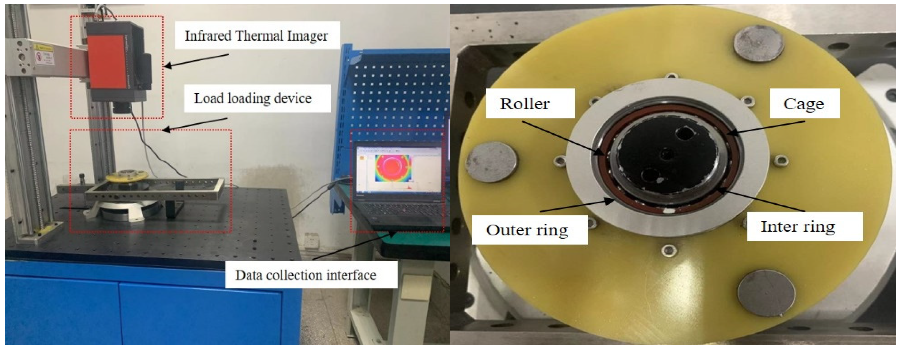
2.1. Experimental Data Sources

The experimental equipment, which includes an infrared thermal imager, bearing axial loading device, and PC-based temperature data acquisition and analysis software, is shown in Figure 1. The experimental bearing was arranged with the end face facing upwards, and the loading was applied as an axial load. The axial force generated by the loading mechanism was first applied to the bearing housing cover and then transferred from the bearing housing cover to the test bearing.

The infrared thermal imager is an ImagelR8355 type; its main technical indicators are temperature measurement range −10~+175 °C, thermal image sampling frequency 10~110 Hz, measurement accuracy ±0.5 °C, thermal sensitivity 20 mK, and infrared image resolution 640 × 512. The rotational speed range of the experimental machine is 0 to 6000 rpm, and the rotational speed control function can be achieved through control software. The axial loading device applies loads ranging from 0 to 30 N. The experimental machine is capable of real-time monitoring of test parameters such as inner ring and cage rotation speed, axial loading load, and contact area temperature between the rolling elements and the inner/outer rings of the experimental bearing and can provide real-time feedback to the display.

The bearing temperature rise experiment process is as follows:

• Preliminary preparation: Assess the condition of the spindle drive device, axial loading device, infrared thermal imager, and other equipment to ensure the safety, reliability, and clear image display in the experimental process.
• Experimental bearing installation: Identify the type of the target bearing for the experiment and proceed with the installation of the experimental bearing.
• Determine the test condition: Establish the preload axial force and motor rotational speed based on the specific objectives of the experiment.
• Data acquisition: Adjust the parameters, such as the emissivity of the infrared thermal imager, set the sampling frequency, and complete the experimental data acquisition.

To ensure the reliability and stability of the experimental results, as well as to eliminate potential chance factors and errors, it was necessary to verify the universal applicability of the obtained data. The experiment was repeated three times at 5000 rpm and with a load of 30 N. The errors between the test results were within 0.5 °C, indicating the reliability of the experiment data.

Dynamic load rating of the bearing C = 200 N was performed according to ISO 281 (C/P) with different axial loads (10 N, 20 N, and 30 N), i.e., load factor C/P (20, 10, and 6.67), combined with various rotational speeds (2000 rpm, 3000 rpm, 4000 rpm, 5000 rpm, and 6000 rpm). Temperature data were collected from the surface of the inner ring of the bearing. Each operating condition was sampled every minute for a duration of one hour.

2.2. Simulation Data Sources

In this paper, a training set was constructed using both simulation and experimental data to predict the temperature rise process of an H7006C angular contact ball bearing under various operating conditions. The main structural parameters of the model object were as follows: inner race diameter (d) of 30 mm, outer race diameter (D) of 55 mm, width (B) of 13 mm, rolling diameter (Dw) of 5.556 mm, number of rolling elements (Z) of 16, contact angle (α) of 15 °, and grease lubrication as the lubrication method. This approach aims to enhance the accuracy and generalization capability of the bearing temperature rise prediction model.

(1)

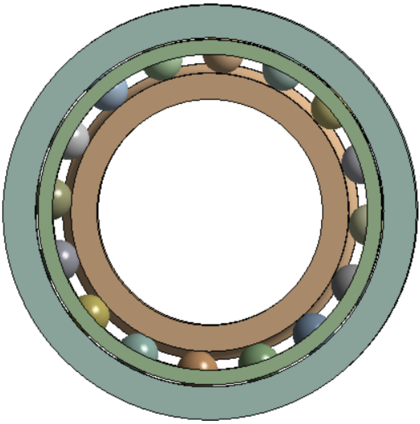
Simulation model

Based on the structural parameters described in the previous section, a three-dimensional model of the H7006C angular contact ball bearing was established, as shown in Figure 2. The material parameters for this bearing are listed in

Table 1. H7006C material parameters.

Parameters	GCr15 (Rings)	Si3N4 (Rollers)	Pi (Cage)
Density	7800	3200	1120
Modulus of elasticity	208	300	300
Poisson’s ratio	0.3	0.26	0.34
Thermal conductivity	40	11	0.15
Specific heat capacity	450	800	1250

Note: Pi represents polyimide, the material utilized for the bearing cage in this study.

.

The transient temperature field simulation process was conducted as follows:

• Model building: Establish a 3D simulation model based on bearing geometry information and material parameters.
• Heat generation calculation: Determine the test conditions and each bearing component’s heat generation.
• Pre-processing: Given the boundary conditions, such as heat convection, heat flow, etc., set the time step and initial temperature.
• Post-processing: Start the transient temperature field simulation, save, and analyze the simulation results.

(2)

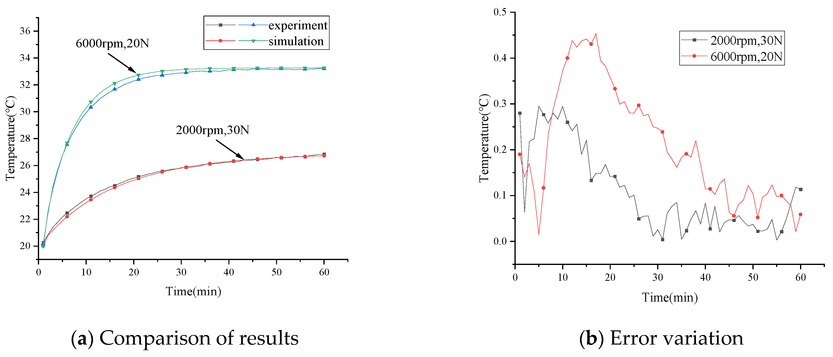
Validation

To ensure the accuracy of the simulation data for the bearing temperature rise process in this paper, the experimental results were compared under two operating conditions: Operating Condition 1 (2000 rpm, 30 N) and Operating Condition 2 (6000 rpm, 20 N). The comparison results are illustrated in Figure 3.

Figure 3 demonstrates that both operating conditions reached a steady-state stage within 30 min, with a temperature change of less than 1 °C. The simulation results align with the experimental results in terms of the temperature rise trend. The slight error in the temperature rise process may be attributed to the neglect of frictional power loss from the cage when constructing the thermal simulation model of the angular contact ball bearing. As a result, the raw heat input to the model was slightly lower than the actual value. However, the temperature error at steady-state was below 0.3 °C in both cases. Generally, a deviation of less than 1 °C under steady-state conditions is considered negligible for the dimensional changes of ball-bearing components. Therefore, the simulation data utilized in this paper can be employed as the training set for the prediction model, enabling the prediction of the bearing temperature rise process.

Dynamic load rating of the bearing C = 200 N was performed according to ISO 281 (C/P) with different axial loads (40 N, 50 N, and 60 N), i.e., load factor C/P (5, 4, and 3.34), combined with various rotational speeds (2000 rpm, 3000 rpm, 4000 rpm, 5000 rpm, and 6000 rpm). Each operating condition was sampled every minute for a duration of one hour in the simulation.

The experimental and simulation data consisted of a total of 30 operating conditions. Among these, the test set was composed of different load factors C/P (20, 10, 6.67, 5, 4, and 3.34) corresponding to a rotational speed of 6000 rpm, and different rotational speeds (2000 rpm, 3000 rpm, 4000 rpm, 5000 rpm, and 6000 rpm) corresponding to a load of 60 N. This test set was specifically utilized for evaluating the performance of the model, while the remaining data were used for pre-training the model.

3. Bearing Temperature Rise Prediction Based on CNN and Informer Combination Method

3.1. Convolutional Neural Networks

Compared to traditional feature extraction methods, CNN usage offers a more effective approach in extracting relevant information from data. In the temperature rise prediction model described in this paper, we employed convolution by taking nested sequence features as input. The key objective of the convolution process involves extracting input feature values through the utilization of a convolution kernel, specifically creating an M × N array. By sliding the kernel with a specific stride, a local matrix is obtained. The convolution kernel transforms this local matrix, resulting in the output matrix for the convolution layer. This convolution process discards certain eigenvalue points while preserving the order relationship among the original input matrix features. Ultimately, it reduces the computational burden on the neural network. The process of convolution operation is as follows:

$$x_l^i=f(x_{l-1}^r\times K_l^i+b_l^i)=f({\displaystyle \sum _r^{}{x}_{l-1}^r\times K_{l,r}^i+b_l^i})$$

(1)

where $x_l^i$ is the feature map output by the i-th convolutional layer $l$, $x_{l-1}^i$ is the r-th convolution region of the feature map generated by convolution layer $l-1$, $K_l^i$ is the weight matrix of the i-th convolution kernel of convolution layer $l$, and $b_l^i$ is the bias value.

Typically, a pooling layer is added after each convolutional layer in order to generate a lower-dimensional feature map and decrease computational complexity. The maximum pooling layer takes the maximum value of features within a certain region as the output, achieving further feature extraction.

3.2. Informer Model

The Informer model is a network architecture built upon an attention mechanism. It primarily enhances the computational efficiency of several components, including the self-attention mechanism, stacked layers of the network, and the incremental decoding method.

The model consists of two parts, an encoder and a decoder, which accept different input data. The encoder is responsible for receiving long sequence data as input. To replace the traditional self-attentive mechanism, it employs a sparse self-attentive mechanism. This modification effectively reduces the network size and enhances the model’s robustness when multiple layers are stacked. On the other hand, the decoder receives input data in the form of long sequences. It fills the target elements with zeros and utilizes these all-zero sequences as part of the weighted attention for the feature map. Subsequently, it utilizes a generative approach to predict the sequences. The calculation of the sparse self-attention mechanism is as follows:

$$A(Q,K,V)=\mathit{Softmax}(\frac{\overline{Q}{K}^T}{\sqrt{D_K}})V$$

(2)

where $\overline{Q}$ is the matrix obtained by probabilistic sparse of $Q$ and $\mathit{Softmax}$ is the normalized activation function.

The encoder employs a “distillation” operation to prioritize the prominent high-level features and generate a concentrated self-attentive feature map in the lower layer, thereby reducing the input length. The “distillation” operation from layer $j$ to layer $j$ + 1 at time $t$ can be described as follows:

$$X_{j+1}^t=\mathit{MaxPool}(\mathit{ELU}(\mathit{Conv}1\mathit{d}{\left[X_j^t\right]}_{\mathit{AB}}))$$

(3)

where ${[\ast ]}_{AB}$ basic operations contain attention blocks and sparse attention mechanisms; $\mathit{Conv}1\mathit{d}$ denotes the one-dimensional convolution operation; $ELU$ is the activation function; and MaxPool is the maximum pooling operation.

The decoder design aims to generate long sequence predictions through a single forward process. The model adopts a traditional Decoder structure, which includes two identical multi-headed attention layers, in order to address the issue of high time complexity involved in generative prediction for long sequential data. The input vector of the decoder is represented as follows:

$$X_{de}^t=Concat(X_{token}^t,X_0^t)\in R^{(L_{token}+L_y)d_{model}}$$

(4)

where $X_{token}^t$ is the start token, and $X_0^t$ is a placeholder for the target sequence, which is set to 0.

3.3. CNN + Informer Bearing Temperature Rise Prediction Model

A CNN and Informer fusion approach was proposed to enhance the accuracy of predicting the bearing temperature rise process. The constructed dataset was utilized as input for the CNN model, employing the same parameters across different regions to calculate convolutional features. This technique reduces the number of parameters in the training process, mitigating the risk of overfitting. Subsequently, through multi-level convolution and pooling operations, the model extracts multi-scale features from the data. These extracted features are then fed into the Informer model via a fully connected layer. The Informer network model is iteratively trained to achieve precise prediction of bearing temperature rise. The structure of the prediction model for bearing temperature rise based on the CNN + Informer fusion is depicted in Figure 4.

The combined prediction model consists of two main parts: two-dimensional convolutional feature extraction and prediction. Initially, the input features of the variables are extracted using two-dimensional convolution, constructing a high-dimensional mapping feature vector. To enhance the feature extraction capability, this study adopted two layers of two-dimensional convolutional layers. The output of the convolutional module is received by both the encoder and decoder parts of the Informer model. The encoder handles long time series data, while the decoder processes short sequences and vectors of equal length comprising zero values as placeholders for predicted values. As the data pass through the encoder, intermediate results are generated through the multi-head sparse self-attentive module and the “distillation” mechanism module, which are computed multiple times in succession. The decoder takes the encoded input data and performs a multi-head sparse self-attentiveness operation with a mask. Subsequently, the intermediate result from the encoder undergoes a multi-head self-attentiveness operation. Finally, a fully connected layer adjusts the dimensionality of the output data and produces the prediction results.

The mean absolute error (MAE) and mean squared error (MSE) are common evaluation metrics for model performance. MAE represents the average error between predicted and true values, calculated as the average of the absolute differences. A smaller MAE indicates a higher accuracy. On the other hand, MSE represents the average of the squared differences between predicted and true values, which assesses the effectiveness of the model. A smaller MSE signifies better performance. In the case of the prediction model for the overall temperature rise process in different bearing operating conditions, the focus lies on the differences between predicted and actual values at each time point. Therefore, this paper utilized MAE as the evaluation metric for accuracy. The specific formula for calculating MAE is as follows:

$$MAE=\frac{1}{n}{\displaystyle \sum _{i=1}^n\left|y_i-y_i^{\ast }\right|}$$

(5)

where n is the number of sample data points; $y_i$ is the true value; and $y_i^{\ast }$ is the predicted value.

4. Results and Discussion

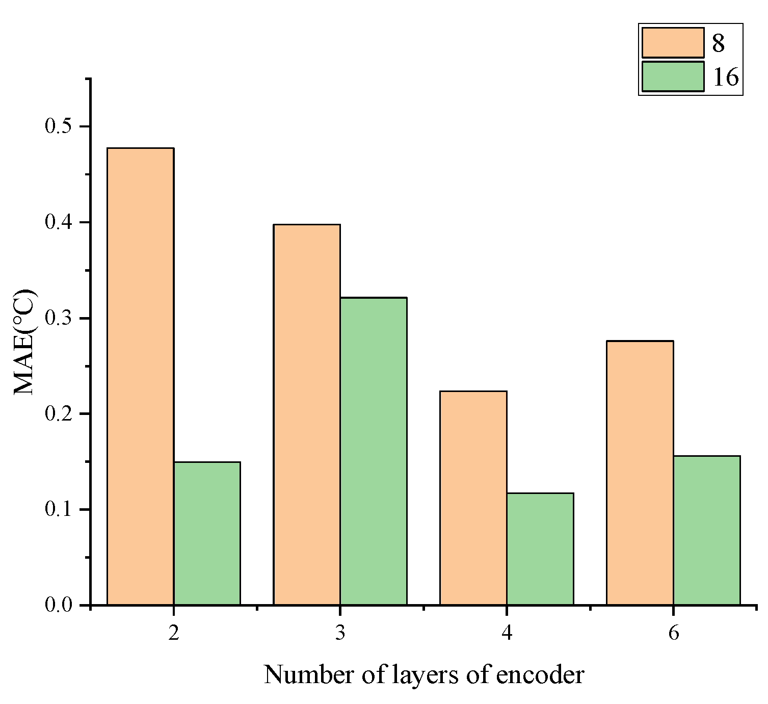
4.1. Parameter Optimization

The experiments were conducted on a Windows 10 system, equipped with an Intel Core i5 processor and an NVIDIA GeForce 930 graphics card.

In the temperature rise prediction model using CNN + Informer, there are several hyperparameters that need to be set separately. In this paper, the parameter selection range is shown in

Table 2. Model parameters.

Parameter Name	Parameter Value
Number of convolution layers	2
Convolution kernel size	3 × 1/2 × 1
Number of convolution kernels	1~10/1~20
Number of encoder layers	3, 4, 6
Number of decoder layers	2
Head number of multi-head attention	8, 16

.

First, the number of encoder layers and the head number of the multi-head attention in Informer were selected as 2 and 8, respectively, to determine the convolution kernel parameters. The convolution kernels for convolution layer 1 range from 1 to 10, and the convolution kernels for convolution layer 2 range from 1 to 20, and partial error data are shown in

Table 3. Comparison of partial errors with different numbers of convolution kernels.

Model	Convolutional Layer 1 Number of Convolutional Kernels	Convolutional Layer 2 Number of Convolutional Kernels	MAE/°C
CNN	1	20	0.6263
	3	1	0.6125
	1	2	0.6005
	2	15	0.5963
	4	1	0.4775

.

Table 3 displays combinations of convolutional kernel counts with relatively smaller errors, and it can be observed that our proposed model achieved the minimum testing error on the dataset when the numbers of convolutional kernels were set to 4 and 1. After determining the convolution kernel parameters, the head number of the multi-head attention and the number of encoder layers for the Informer model were set accordingly. The resulting error outcomes are illustrated in Figure 5.

Based on the findings in Figure 5, when the head number of the multi-head attention was set to 16, there were smaller errors across different encoder layers compared to when it was set to 8. Notably, the model’s error was minimized when the number of encoder layers was specified as 4. Consequently, the structure of the temperature rise prediction model using the CNN + Informer approach was determined, and the specific parameters are outlined in

Table 4. CNN + Informer model parameters.

Model	Parameter Name	Parameter Value
CNN	Number of convolution layers	2
	Convolution kernel size	3 × 1/2 × 1
	Number of convolution kernels	4/1
Informer	Number of encoder layers	4
	Number of decoder layers	2
	Head number of multi-head attention	16

.

4.2. Comparison and Analysis of Prediction Results

Based on the previous analysis, it was observed that the bearing temperature, under different working conditions, generally reached a steady-state at around the 30 min mark. To evaluate the prediction capability of the proposed CNN + Informer model, we constructed models using LSTM, Informer, and CNN + Informer. The errors during both the temperature rise stage and the steady-state stage were compared among these models.

4.2.1. Model Prediction Results with Varying Rotational Speeds

The predictions of the multiple models under a rotational speed of 5000 rpm and a load of 60 N are presented in Figure 6. Furthermore, Figure 7 showcases the variations in prediction errors throughout the temperature rise and steady-state stages at various rotational speeds (2000 rpm, 3000 rpm, 4000 rpm, 5000 rpm, and 6000 rpm).

Based on the comparison of the model prediction results presented in Figure 6a, it can be observed that both the Informer and LSTM models exhibited varying degrees of fluctuation in their prediction results. In contrast, the model used in this paper demonstrated a consistent upward trend that closely aligned with the actual values, resembling the real curve more closely. Furthermore, Figure 6b illustrates a comparison of the prediction errors. It is evident that the maximum error of the model proposed in this paper remained within 0.5 °C, whereas the maximum error of the other two models exceeded 1 °C.

From Figure 7, it is evident that the model used in this paper exhibited lower prediction errors compared to the other two models at the various rotational speeds. The average absolute error of the predictions made by this model consistently remained below 0.2 °C. Furthermore, there is no discernible trend in the change of prediction errors as the rotational speed increased. This indicates that the model demonstrates good stability and is capable of accurately predicting temperature rise under varying rotational speeds.

4.2.2. Model Prediction Results with Varying Load

When the bearing rotational speed is 6000 rpm, Figure 8 depicts the prediction results of the multiple models for a load of 50 N. Meanwhile, Figure 9 demonstrates the prediction errors during both the temperature rise phase and steady-state phase under various loads (10 N, 20 N, 30 N, 40 N, and 50 N).

The comparison of the prediction results in Figure 8a reveals a gradual deviation between the predictions of the Informer and LSTM models from the actual values over time. Figure 8b shows the error between predictions from Informer and LSTM models and the actual values gradually grows over time. In contrast, the model utilized in this paper consistently maintained an error within 0.5 °C without any discernible trend over time.

The prediction errors of the model under different loads in Figure 9 indicate that its error consistently remained within 0.5 °C, which is lower compared to the other two models. Moreover, as the load increased, there is no clear upward trend observed in the prediction errors of this model during both the temperature rise and steady-state stages. This suggests that the model exhibits high prediction accuracy and good stability.

4.2.3. Experimental Data Prediction Results and Analysis

Figure 10 depicts the evaluation of the model using the predicted results of the experimental data. In Figure 10a, it is evident that the error in the model’s prediction results was more pronounced during the temperature rise stage. However, it can be observed that the error gradually decreased over time. Additionally, Figure 10b displays the error under various working conditions, indicating that the maximum error remained within 0.2 °C. This demonstrates the high accuracy of the model and verifies its prediction capability and reliability as presented in this paper.

4.3. Generalization Ability Experiment

To evaluate the generalization ability of the model, its prediction results were observed and evaluated under various operating conditions that were not included in the original dataset. The dataset includes simulation data under different room temperature conditions. As depicted in Figure 11, the model demonstrated good prediction performance when tested with new conditions through both empirical testing and simulations. The predicted curves gradually approached the true curve, indicating accurate predictions. When reaching the steady state, the deviation between the prediction curve and the true value was less than 0.5 °C, and the error during the steady-state stage was lower compared to that during the temperature rise stage. This could be attributed to the stabilization of the heat generation and dissipation processes during the steady-state stage, whereby this equilibrium state contributes to a reduction in prediction errors.

The results of the prediction and error analysis under different operating conditions demonstrated the accuracy of the temperature rise prediction model used in this paper for various rotational speed and load conditions. The proposed model exhibited lower errors compared to two other models, both during the temperature rise stage and the steady-state stage, confirming its validity and performance. Moreover, as the rotational speed and load increased, there is no noticeable trend in the prediction error, indicating the excellent stability of the model. Furthermore, the model demonstrated favorable prediction results for operating conditions not included in the original dataset, providing further evidence of its generalization ability. In summary, our research demonstrated that the predictive model exhibits a consistent trend with the true values, and there is no delay issue in its predictions. This enables real-time bearing condition monitoring, facilitating proactive maintenance strategies and ensuring efficient and reliable operation of rotating machinery.

5. Conclusions

This study proposed a temperature rise prediction method based on deep learning models for spindle bearings in the high-speed operating conditions of machine tools. The method was developed to address challenges associated with timely assessment of bearing conditions due to rapid temperature changes. The specific conclusions are as follows:

(1)

The proposed simulation model for the temperature field of angular contact ball bearings demonstrated an error of less than 0.5 °C when compared to the experimental results. This finding suggests that the simulation data exhibit high reliability and fulfill the requirements for training samples in the prediction model.

(2)

Compared to LSTM and Informer, the optimized CNN + Informer model achieved higher accuracy and prediction stability. It achieved errors within 0.5 °C for multiple operating conditions and showed no variation trend with changing operating conditions.

(3)

For operating conditions outside the dataset, the model predicted errors within 0.5 °C and 0.2 °C during the temperature rise and steady-state stages, respectively. This suggests that the prediction error decreases over time, providing further evidence for the model’s generalization ability and effectiveness.

References

- Ma, S.; Yin, Y.; Chao, B.; Yan, K.; Fang, B.; Hong, J. A Real-time Coupling Model of Bearing-Rotor System Based on Semi-flexible Body Element. Int. J. Mech. Sci. 2023, 245, 108098. [Google Scholar] [CrossRef]
- Fang, B.; Zhang, J.; Hong, J.; Yan, K. Research on the nonlinear stiffness characteristics of double-row angular contact ball bearings under different working conditions. Lubricants 2023, 11, 44. [Google Scholar] [CrossRef]
- Popescu, A.; Houpert, L.; Olaru, D.N. Four approaches for calculating power losses in an angular contact ball bearing. Mech. Mach. Theory 2020, 144, 103669. [Google Scholar] [CrossRef]
- Kim, K.-S.; Lee, D.-W.; Lee, S.-M.; Hwang, J.-H. A numerical approach to determine the frictional torque and temperature of an angular contact ball bearing in a spindle system. Int. J. Precis. Eng. Manuf. 2015, 16, 135–142. [Google Scholar] [CrossRef]
- Xu, J.; Zhang, J.; Huang, Z.; Wang, L. Calculation and finite element analysis of the temperature field for high-speed rail bearing based on vibrational characteristics. J. Vibroeng. 2015, 17, 720–732. [Google Scholar]
- Deng, X.; Fu, J.; Zhang, Y. A predictive model for temperature rise of spindle–bearing integrated system. J. Manuf. Sci. Eng. 2015, 137, 021014. [Google Scholar] [CrossRef]
- Wu, L.; Tan, Q. Thermal characteristic analysis and experimental study of a spindle-bearing system. Entropy 2016, 18, 271. [Google Scholar] [CrossRef]
- Zheng, D.; Chen, W.F. Effect of structure and assembly constraints on temperature of high-speed angular contact ball bearings with thermal network method. Mech. Syst. Signal Process. 2020, 145, 106929. [Google Scholar] [CrossRef]
- Li, Z.; Zhao, C.; Lu, Z.; Liu, F. Thermal Performances Prediction Analysis of High Speed Feed Shaft Bearings Under Actual Working Condition. IEEE Access 2019, 7, 168011–168019. [Google Scholar] [CrossRef]
- Zhang, C.; Guo, D.; Tian, J.; Niu, Q. Research on the influencing factors of thermal characteristics of high-speed grease lubricated angular contact ball bearing. Adv. Mech. Eng. 2021, 13, 16878140211027398. [Google Scholar] [CrossRef]
- Yan, G.; Yu, C.; Bai, Y. Wind turbine bearing temperature forecasting using a new data-driven ensemble approach. Machines 2021, 9, 248. [Google Scholar] [CrossRef]
- Liu, Y.Z.; Zou, Y.S.; Wu, Y. A novel abnormal detection method for bearing temperature based on spatiotemporal fusion. Proc. Inst. Mech. Eng. Part F J. Rail Rapid Transit 2022, 236, 317–333. [Google Scholar] [CrossRef]
- Chen, Y.; Zhang, C.; Zhang, N.; Chen, Y. Multi-task learning and attention mechanism based long short-term memory for temperature prediction of EMU bearing. In Proceedings of the 2019 Prognostics and System Health Management Conference (PHM-Qingdao), Qingdao, China, 25–27 October 2019; pp. 1–7. [Google Scholar]
- Xiao, X.; Liu, J.; Liu, D.; Tang, Y.; Dai, J.; Zhang, F. SSAE—MLP: Stacked sparse autoencoders-based multi-layer perceptron for main bearing temperature prediction of large-scale wind turbines. Concurr. Comput. Pract. Exp. 2021, 33, e6315. [Google Scholar] [CrossRef]
- Ariyo, A.A.; Adewumi, A.O.; Ayo, C.K. Stock price prediction using the ARIMA model. In Proceedings of the 2014 UKSim-AMSS 16th International Conference on Computer Modelling and Simulation, Cambridge, UK, 26–28 March 2014; pp. 106–112. [Google Scholar]
- Zhang, Y.; Sun, H.; Guo, Y. Wind power prediction based on PSO-SVR and grey combination model. IEEE Access 2019, 7, 136254–136267. [Google Scholar] [CrossRef]
- Cui, K.; Jing, X. Research on prediction model of geotechnical parameters based on BP neural network. Neural Comput. Appl. 2019, 31, 8205–8215. [Google Scholar] [CrossRef]
- Lukoševičius, M.; Jaeger, H. Reservoir computing approaches to recurrent neural network training. Comput. Sci. Rev. 2009, 3, 127–149. [Google Scholar] [CrossRef]
- Yu, Y.; Si, X.; Hu, C.; Zhang, J. A review of recurrent neural networks: LSTM cells and network architectures. Neural Comput. 2019, 31, 1235–1270. [Google Scholar] [CrossRef]
- Fan, C.; Zhang, Y.; Pan, Y.; Li, X.; Zhang, C.; Yuan, R.; Wu, D.; Wang, W.; Pei, J.; Huang, H. Multi-horizon time series forecasting with temporal attention learning. In Proceedings of the 25th ACM SIGKDD International Conference on Knowledge Discovery & Data Mining, Anchorage, AK, USA, 4–8 August 2019; pp. 2527–2535. [Google Scholar]
- Zhou, H.; Zhang, S.; Peng, J.; Zhang, S.; Li, J.; Xiong, H.; Zhang, W. Informer: Beyond efficient transformer for long sequence time-series forecasting. In Proceedings of the AAAI Conference on Artificial Intelligence, Virtual, 2–9 February 2021; Volume 35, pp. 11106–11115. [Google Scholar]
- Gong, M.; Zhao, Y.; Sun, J.; Han, C.; Sun, G.; Yan, B. Load forecasting of district heating system based on Informer. Energy 2022, 253, 124179. [Google Scholar] [CrossRef]
- Yang, Z.; Liu, L.; Li, N.; Tian, J. Time series forecasting of motor bearing vibration based on informer. Sensors 2022, 22, 5858. [Google Scholar] [CrossRef] [PubMed]