Characterisation of the Contact between Cross-Country Skis and Snow: A Micro-Scale Study Considering the Ski-Base Texture

 , , ,
, , , 
Abstract
1. Introduction
2. Theory
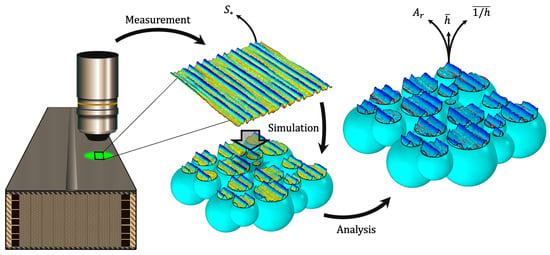
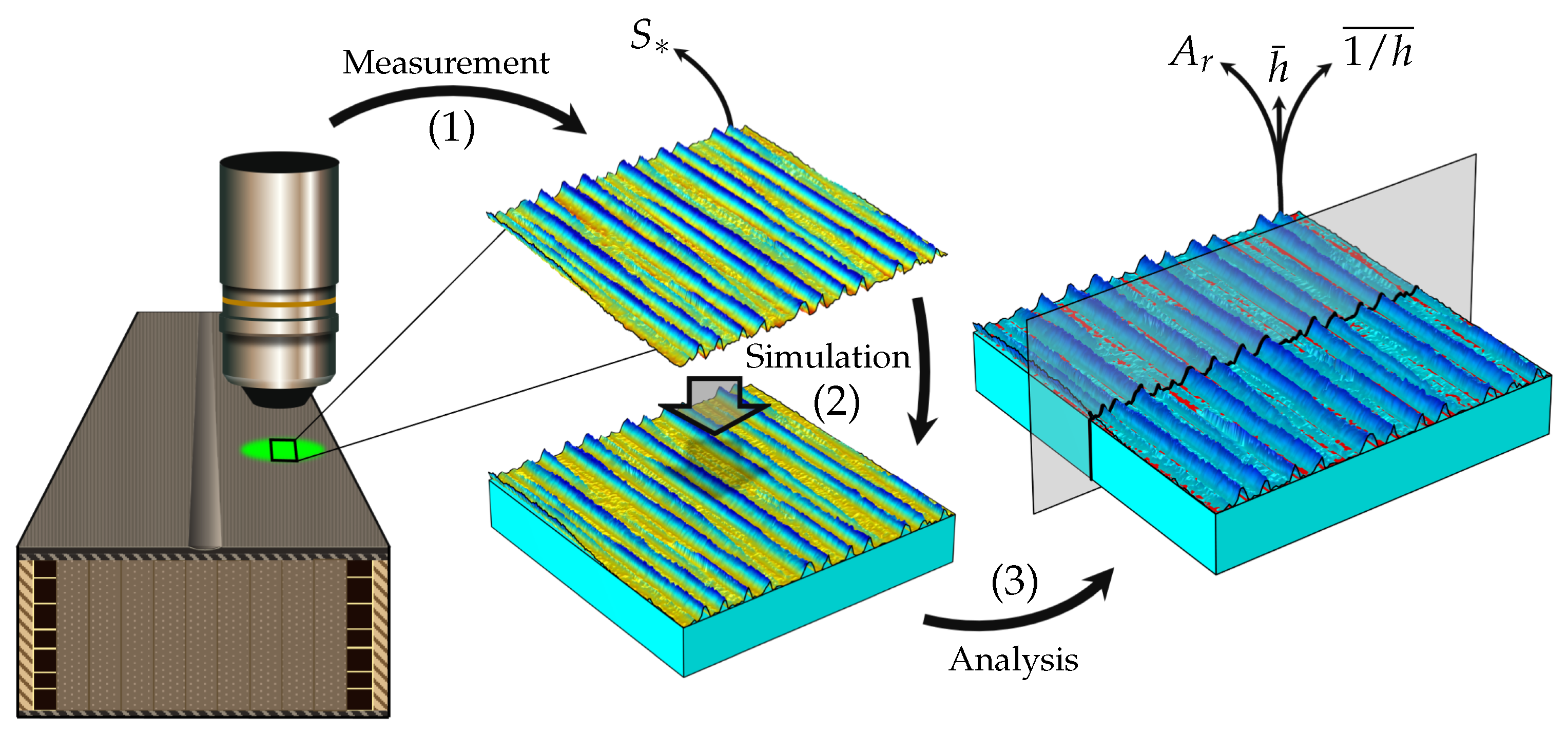
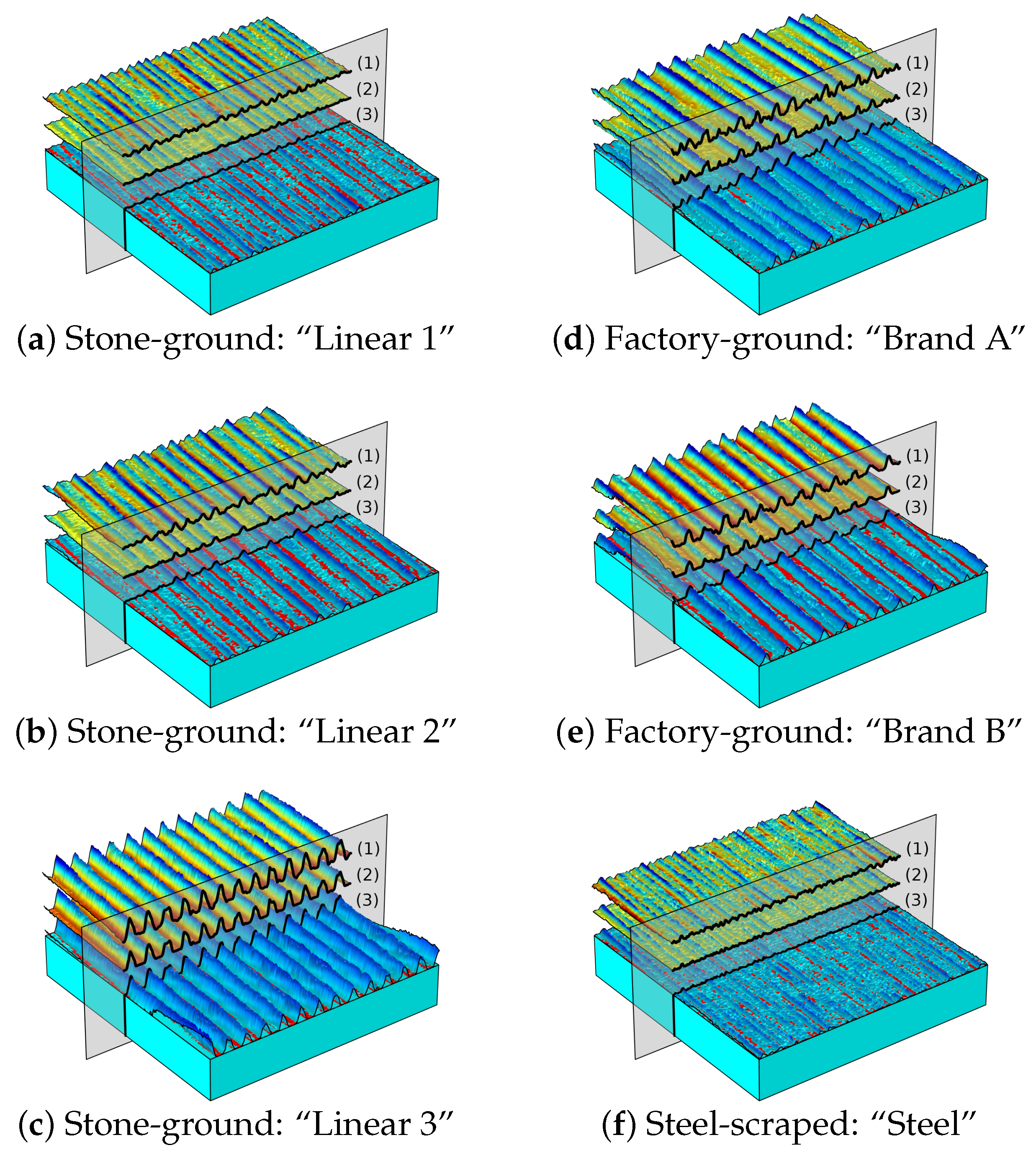
3. Method
4. Results and Discussion
4.1. Standardised Surface Roughness Parameters
4.2. Functional Parameters
4.3. Comparison with Previous Results
4.3.1. Rohm et al.
4.3.2. Scherge et al.
4.4. Summary of the Results
5. Conclusions
- Surfaces with higher values have lower contact area, but the alone cannot be used to precisely predict the contact area.
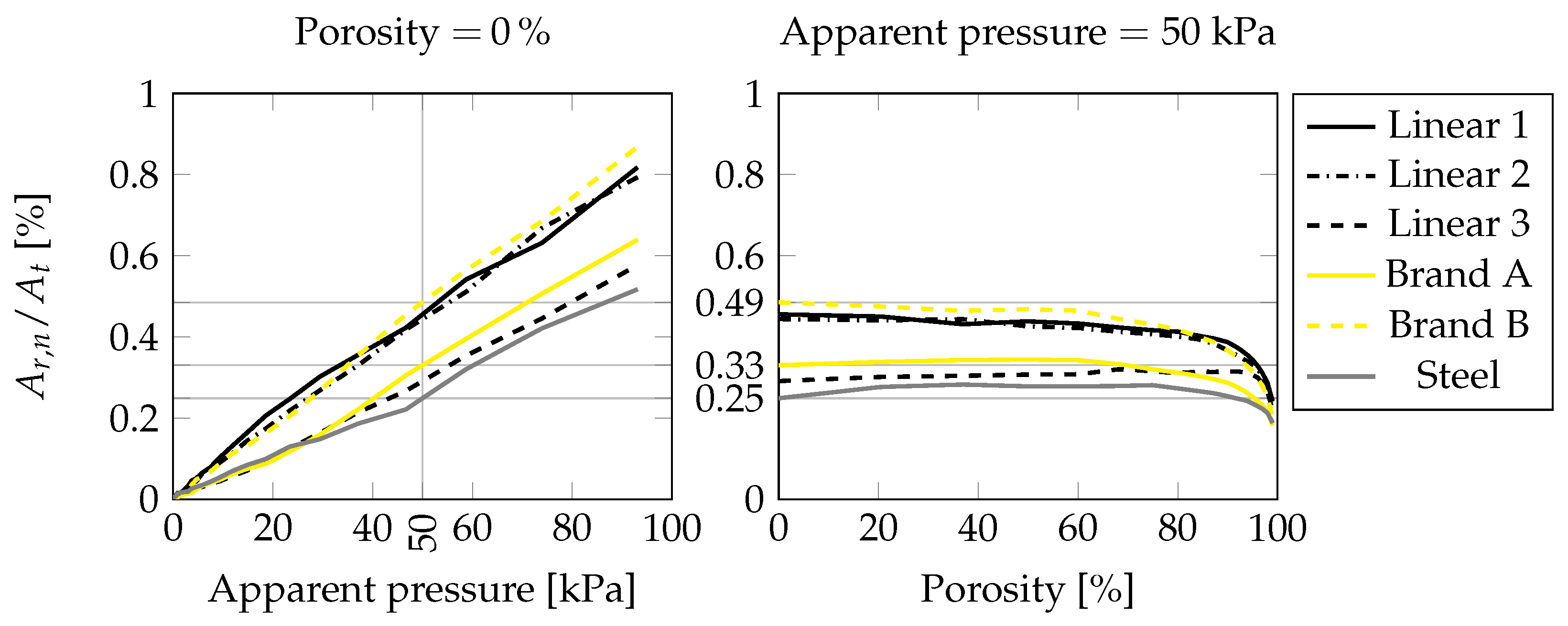
- It was found that an increase in the porosity decreased the real area of contact, and ski-base textures with a larger real area of contact at exhibited a higher variability.
- The surfaces were grouped by their values and the group with the lower values showed a higher rate of increase in contact area with increasing apparent pressure.
- The relative differences between the real area of contact for the Linear 3 (“roughest”) and the steel-scraped surface (“smoothest”), and between the Linear 1 (second “smoothest”) and the steel-scraped surface, at an apparent pressure of 50 , were found to be ≈32% and ≈84%, respectively, indicating that the value is not correlated with the real area of contact.
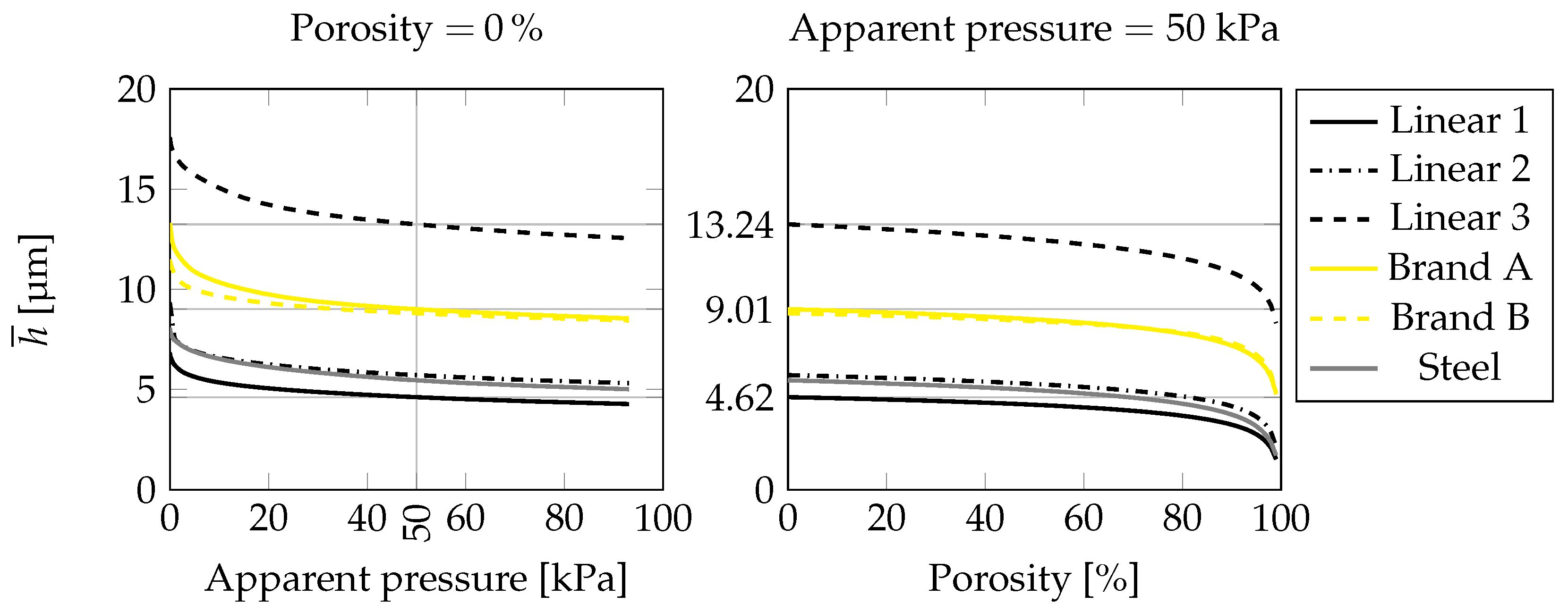
- The differences between the average interfacial separation for the steel-scraped (“smoothest”) and the Linear 3 surfaces (“roughest”), and the steel-scraped (“smoothest”) and the Linear 1 surfaces (second “smoothest”), at a 50 apparent pressure, were found to be ≈300% and ≈17%, respectively.
- The reciprocal average interfacial separation, hence the viscous part of the friction, is expected to be ≈50% higher for the Linear 1 than for the Linear 3 texture at a 50 apparent pressure.
- The viscous friction is linearly dependent on the velocity and the reciprocal average interfacial separation (), and is larger for the Linear 1 texture than for all the other five surfaces considered here.
- The reciprocal average interfacial separation can be used to compare textures and possibly help to discern whether a texture performs well under warm conditions or not.
Author Contributions
Funding
Data Availability Statement
Acknowledgments
Conflicts of Interest
Nomenclature
| Elastic modulus of ice = 9 ( ) | |
| Elastic modulus of the ski base = ( ) | |
| Unconfined compressive strength ( ) | |
| Poisson ratio | |
| Pore surface area ( 2) | |
| Total surface area ( 2) | |
| Real area of contact for a nonporous surface ( 2) | |
| Real area of contact for a porous surface (2) | |
| Computational domain | |
| The part of the domain where there is contact | |
| The part of the domain where there is a gap (not contact) | |
| U | Sliding velocity ( −1) |
| n | Surface porosity |
| p | Nominal load ( ) |
| Apparent pressure ( ) | |
| P | Load ( ) |
| Rigid body displacement ( ) | |
| h | Interfacial separation ( ) |
| Average interfacial separation ( ) | |
| Average reciprocal interfacial separation ( −1) | |
| Surface roughness parameters | |
| Arithmetic mean deviation | |
| Root-mean-square deviation | |
| Skewness | |
| Kurtosis | |
| Root-mean-square slope | |
| Reduced peak height | |
| Core roughness depth | |
| Reduced valley height |
References
- Almqvist, A.; Pellegrini, B.; Lintzén, N.; Emami, N.; Holmberg, H.C.; Larsson, R. A Scientific Perspective on Reducing Ski-Snow Friction to Improve Performance in Olympic Cross-Country Skiing, the Biathlon and Nordic Combined. Front. Sport. Act. Living 2022, 4, 844883. [Google Scholar] [CrossRef] [PubMed]
- Street, G.M.; Gregory, R.W. Relationship between Glide Speed and Olympic Cross-Country Ski Performance. J. Appl. Biomech. 1994, 10, 393–399. [Google Scholar] [CrossRef]
- Bowden, F.; Hughes, T. The mechanism of sliding on ice and snow. Proc. R. Soc. Lond. Ser. A Math. Phys. Sci. 1939, 172, 280–298. [Google Scholar] [CrossRef]
- Eriksson, R. Friction of runners on snow and ice. Meddelanden från Föreningen Skogsarbetens och Kungl. Domänstyrelsens Arbetsstudieavdelning 1949, 35, 25–63. [Google Scholar]
- Bowden, F.P. Some Recent Experiments in Friction: Friction on Snow and Ice and the Development of some Fast-Running Skis. Nature 1955, 176, 946–947. [Google Scholar] [CrossRef]
- Lever, J.H.; Asenath-Smith, E.; Taylor, S.; Lines, A.P. Assessing the Mechanisms Thought to Govern Ice and Snow Friction and Their Interplay With Substrate Brittle Behavior. Front. Mech. Eng. 2021, 7, 690425. [Google Scholar] [CrossRef]
- Glenne, B. Sliding Friction and Boundary Lubrication of Snow. J. Tribol. 1987, 109, 614–617. [Google Scholar] [CrossRef]
- Makkonen, L. Application of a new friction theory to ice and snow. Ann. Glaciol. 1994, 19, 155–157. [Google Scholar] [CrossRef]
- Aghababaei, R.; Brodsky, E.E.; Molinari, J.F.; Chandrasekar, S. How Roughness Emerges on Natural and Engineered Surfaces. MRS Bull. 2023, 47, 1229–1236. [Google Scholar] [CrossRef]
- Lehtovaara, A. Kinetic Friction between Ski and Snow. In Acta Polytechnica Scandinavica: ME; Finnish Academy of Technology: Helsinki, Finland, 1989; Volume 93, pp. 1–52. [Google Scholar]
- Bejan, A. The Fundamentals of Sliding Contact Melting and Friction. J. Heat Transf. 1989, 111, 13–20. Available online: http://xxx.lanl.gov/abs/https://asmedigitalcollection.asme.org/heattransfer/article-pdf/111/1/13/5910218/13_1.pdf (accessed on 10 April 2023). [CrossRef]
- Bejan, A. Contact Melting Heat Transfer and Lubrication. In Advances in Heat Transfer; Elsevier: Amsterdam, The Netherlands, 1994; Volume 24, pp. 1–38. [Google Scholar] [CrossRef]
- Kalliorinne, K.; Hindér, G.; Sandberg, J.; Larsson, R.; Holmberg, H.C.; Almqvist, A. The impact of cross-country skiers’ tucking position on ski-camber profile, apparent contact area and load partitioning. Proc. Inst. Mech. Eng. Part P J. Sport. Eng. Technol. 2023. [Google Scholar] [CrossRef]
- Kalliorinne, K.; Sandberg, J.; Hindér, G.; Larsson, R.; Holmberg, H.C.; Almqvist, A. Characterisation of the Contact between Cross-Country Skis and Snow: A Macro-Scale Investigation of the Apparent Contact. Lubricants 2022, 10, 279. [Google Scholar] [CrossRef]
- Lever, J.H.; Taylor, S.; Hoch, G.R.; Daghlian, C. Evidence that abrasion can govern snow kinetic friction. J. Glaciol. 2019, 65, 68–84. [Google Scholar] [CrossRef]
- Scherge, M.; Stoll, M.; Moseler, M. On the influence of microtopography on the sliding performance of cross country skis. Front. Mech. Eng. 2021, 7, 659995. [Google Scholar] [CrossRef]
- Giesbrecht, J.L.; Smith, P.; Tervoort, T.A. Polymers on snow: Toward skiing faster. J. Polym. Sci. Part B Polym. Phys. 2010, 48, 1543–1551. [Google Scholar] [CrossRef]
- Rohm, S.; Kno, C.; Hasler, M.; Kaserer, L.; van Putten, J.; Unterberger, S.H.; Lackner, R. Effect of Different Bearing Ratios on the Friction between Ultrahigh Molecular Weight Polyethylene Ski Bases and Snow. ACS Appl. Mater. Interfaces 2016, 8, 12552–12557. [Google Scholar] [CrossRef]
- Persson, B.N.J. Functional properties of rough surfaces from an analytical theory of mechanical contact. MRS Bull. 2022, 47, 1211–1219. [Google Scholar] [CrossRef]
- Bäurle, L.; Kaempfer, T.; Szabó, D.; Spencer, N. Sliding friction of polyethylene on snow and ice: Contact area and modeling. Cold Reg. Sci. Technol. 2007, 47, 276–289. [Google Scholar] [CrossRef]
- Theile, T.; Szabo, D.; Luthi, A.; Rhyner, H.; Schneebeli, M. Mechanics of the Ski–Snow Contact. Tribol. Lett. 2009, 36, 223–231. [Google Scholar] [CrossRef]
- Rohm, S.; Unterberger, S.; Hasler, M.; Gufler, M.; van Putten, J.; Lackner, R.; Nachbauer, W. Wear of ski waxes: Effect of temperature, molecule chain length and position on the ski base. Wear 2017, 384–385, 43–49. [Google Scholar] [CrossRef]
- Mössner, M.; Hasler, M.; Nachbauer, W. Calculation of the contact area between snow grains and ski base. Tribol. Int. 2021, 163, 107183. [Google Scholar] [CrossRef]
- Jolivet, S.; Mezghani, S.; El Mansori, M. Multiscale analysis of replication technique efficiency for 3D roughness characterization of manufactured surfaces. Surf. Topogr. Metrol. Prop. 2016, 4, 035002. [Google Scholar] [CrossRef]
- Almqvist, A.; Sahlin, F.; Larsson, R.; Glavatskih, S. On the dry elasto-plastic contact of nominally flat surfaces. Tribol. Int. 2007, 40, 574–579. [Google Scholar] [CrossRef]
- Sahlin, F.; Larsson, R.; Almqvist, A.; Lugt, P.M.; Marklund, P. A mixed lubrication model incorporating measured surface topography. Part 1: Theory of flow factors. Proc. Inst. Mech. Eng. Part J Eng. Tribol. 2010, 224, 335–351. [Google Scholar] [CrossRef]
- Almqvist, A.; Campana, C.; Prodanov, N.; Persson, B.N.J. Interfacial Separation between Elastic Solids with Randomly Rough Surfaces: Comparison between Theory and Numerical Techniques. J. Mech. Phys. Solids 2011, 59, 2355–2369. [Google Scholar] [CrossRef]
- Tiwari, A.; Almqvist, A.; Persson, B.N.J. Plastic Deformation of Rough Metallic Surfaces. Tribol. Lett. 2020, 68, 129. [Google Scholar] [CrossRef]
- Pérez-Ràfols, F.; Almqvist, A. On the Stiffness of Surfaces with Non-Gaussian Height Distribution. Sci. Rep. 2021, 11, 1863. [Google Scholar] [CrossRef]
- Kalliorinne, K.; Larsson, R.; Pérez-Ràfols, F.; Liwicki, M.; Almqvist, A. Artificial Neural Network Architecture for Prediction of Contact Mechanical Response. Front. Mech. Eng. 2021, 6, 579825. [Google Scholar] [CrossRef]
- Persson, B.N.J. On the Use of Surface Roughness Parameters. Tribol. Lett. 2023, 71, 29. [Google Scholar] [CrossRef]
- Bottiglione, F.; Carbone, G.; Persson, B.N.J. Fluid contact angle on solid surfaces: Role of multiscale surface roughness. J. Chem. Phys. 2015, 143, 134705. [Google Scholar] [CrossRef]
- Abbott, E.J.; Firestone, F.A. Specifying Surface Quality: A Method Based on Accurate Measurement and Comparison. J. Mech. Eng. 1933, 59, 569–572. [Google Scholar]
- University of Michigan, College of Engineering. College of Engineering: Announcement 1934–1935 and 1935–1936; University of Michigan: Ann Arbor, MI, USA, 1934; Volume 35. [Google Scholar]
- Persson, B.N.J. Contact mechanics for randomly rough surfaces. Surf. Sci. Rep. 2006, 61, 201–227. [Google Scholar] [CrossRef]
- Persson, B.N.J. Relation between Interfacial Separation and Load: A General Theory of Contact Mechanics. Phys. Rev. Lett. 2007, 99, 125502. [Google Scholar] [CrossRef]
- Yang, C.; Persson, B.N.J. Contact mechanics: Contact area and interfacial separation from small contact to full contact. J. Phys. Condens. Matter 2008, 20, 215214. [Google Scholar] [CrossRef]
- Tada, T.; Kawasaki, S.; Shimizu, R.; Persson, B.N.J. Rubber-ice friction. Friction 2023. [Google Scholar] [CrossRef]


| Textures | (m) | (m) | (-) | (-) | (m/mm) | (m) | (m) | (m) |
|---|---|---|---|---|---|---|---|---|
| Linear 1 | 1.767 | 2.159 | −0.16 | 2.58 | 65.79 | 1.444 | 6.009 | 1.920 |
| Linear 2 | 2.437 | 3.011 | −0.49 | 2.89 | 72.70 | 1.571 | 7.837 | 3.546 |
| Linear 3 | 8.768 | 9.622 | −0.43 | 1.63 | 185.77 | 2.161 | 11.651 | 20.019 |
| Brand A | 4.999 | 6.305 | −1.13 | 3.49 | 168.46 | 1.917 | 9.416 | 13.196 |
| Brand B | 4.881 | 5.803 | −0.58 | 2.38 | 112.82 | 1.217 | 12.695 | 7.965 |
| Steel | 1.693 | 2.126 | −0.09 | 3.34 | 94.25 | 1.925 | 5.499 | 2.149 |
| Textures | (m) | (m) | (m) | (m) |
|---|---|---|---|---|
| Ski 1 | 3.60 | 1.40 | 9.00 | 6.55 |
| Ski 2 | 3.48 | 2.20 | 12.60 | 2.80 |
| Linear 1 | 1.77 | 1.44 | 6.01 | 1.92 |
| Linear 2 | 2.44 | 1.57 | 7.84 | 3.55 |
| Linear 3 | 8.77 | 2.16 | 11.65 | 20.02 |
| Brand A | 5.00 | 1.92 | 9.42 | 13.20 |
| Brand B | 4.88 | 1.22 | 12.70 | 7.97 |
| Steel | 1.69 | 1.93 | 5.50 | 2.15 |
| Textures | (m) | ||||
|---|---|---|---|---|---|
| Ski 1 | 8.3% | 53.1% | 38.6% | 72.8% | 16.95 |
| Ski 2 | 12.5% | 71.6% | 15.9% | 22.2% | 17.60 |
| Linear 1 | 15.4% | 64.1% | 20.5% | 32.0% | 9.37 |
| Linear 2 | 12.1% | 60.5% | 27.4% | 45.2% | 12.95 |
| Linear 3 | 6.4% | 34.4% | 59.2% | 171.8% | 33.83 |
| Brand A | 7.8% | 38.4% | 53.8% | 140.1% | 24.53 |
| Brand B | 5.6% | 58.0% | 36.4% | 62.7% | 21.88 |
| Steel | 20.1% | 57.4% | 22.4% | 39.1% | 9.57 |
| Textures | (m) | (-) | (-) | (m/mm) |
|---|---|---|---|---|
| S1 linear/fine | 1.86 | 0.41 | 1.68 | 135 |
| S2 linear/medium | 1.63 | 0.54 | 2.83 | 107 |
| S3 linear/coarse | 2.84 | 0.18 | 0.33 | 137 |
| S4 linear/mutliple | 2.45 | 0.29 | 0.70 | 175 |
| S5 cross-hatched | 1.81 | 0.67 | 2.22 | 126 |
| Linear 1 | 1.77 | −0.16 | 2.58 | 66 |
| Linear 2 | 2.44 | −0.49 | 2.89 | 73 |
| Linear 3 | 8.77 | −0.43 | 1.63 | 186 |
| Brand A | 5.00 | −1.13 | 3.49 | 168 |
| Brand B | 4.88 | −0.58 | 2.38 | 113 |
| Steel | 1.69 | −0.09 | 3.34 | 94 |
Disclaimer/Publisher’s Note: The statements, opinions and data contained in all publications are solely those of the individual author(s) and contributor(s) and not of MDPI and/or the editor(s). MDPI and/or the editor(s) disclaim responsibility for any injury to people or property resulting from any ideas, methods, instructions or products referred to in the content. |
© 2023 by the authors. Licensee MDPI, Basel, Switzerland. This article is an open access article distributed under the terms and conditions of the Creative Commons Attribution (CC BY) license (https://creativecommons.org/licenses/by/4.0/).
Share and Cite
Kalliorinne, K.; Persson, B.N.J.; Sandberg, J.; Hindér, G.; Larsson, R.; Holmberg, H.-C.; Almqvist, A. Characterisation of the Contact between Cross-Country Skis and Snow: A Micro-Scale Study Considering the Ski-Base Texture. Lubricants 2023, 11, 225. https://doi.org/10.3390/lubricants11050225
Kalliorinne K, Persson BNJ, Sandberg J, Hindér G, Larsson R, Holmberg H-C, Almqvist A. Characterisation of the Contact between Cross-Country Skis and Snow: A Micro-Scale Study Considering the Ski-Base Texture. Lubricants. 2023; 11(5):225. https://doi.org/10.3390/lubricants11050225
Chicago/Turabian StyleKalliorinne, Kalle, Bo N. J. Persson, Joakim Sandberg, Gustav Hindér, Roland Larsson, Hans-Christer Holmberg, and Andreas Almqvist. 2023. "Characterisation of the Contact between Cross-Country Skis and Snow: A Micro-Scale Study Considering the Ski-Base Texture" Lubricants 11, no. 5: 225. https://doi.org/10.3390/lubricants11050225
APA StyleKalliorinne, K., Persson, B. N. J., Sandberg, J., Hindér, G., Larsson, R., Holmberg, H.-C., & Almqvist, A. (2023). Characterisation of the Contact between Cross-Country Skis and Snow: A Micro-Scale Study Considering the Ski-Base Texture. Lubricants, 11(5), 225. https://doi.org/10.3390/lubricants11050225