Evaluation of Various Shear-Thinning Models for Squalane Using Traction Measurements, TEHD and NEMD Simulations


Abstract
1. Introduction
1.1. Viscosity
1.2. Shear-Thinning
1.2.1. Option I—Rheometry
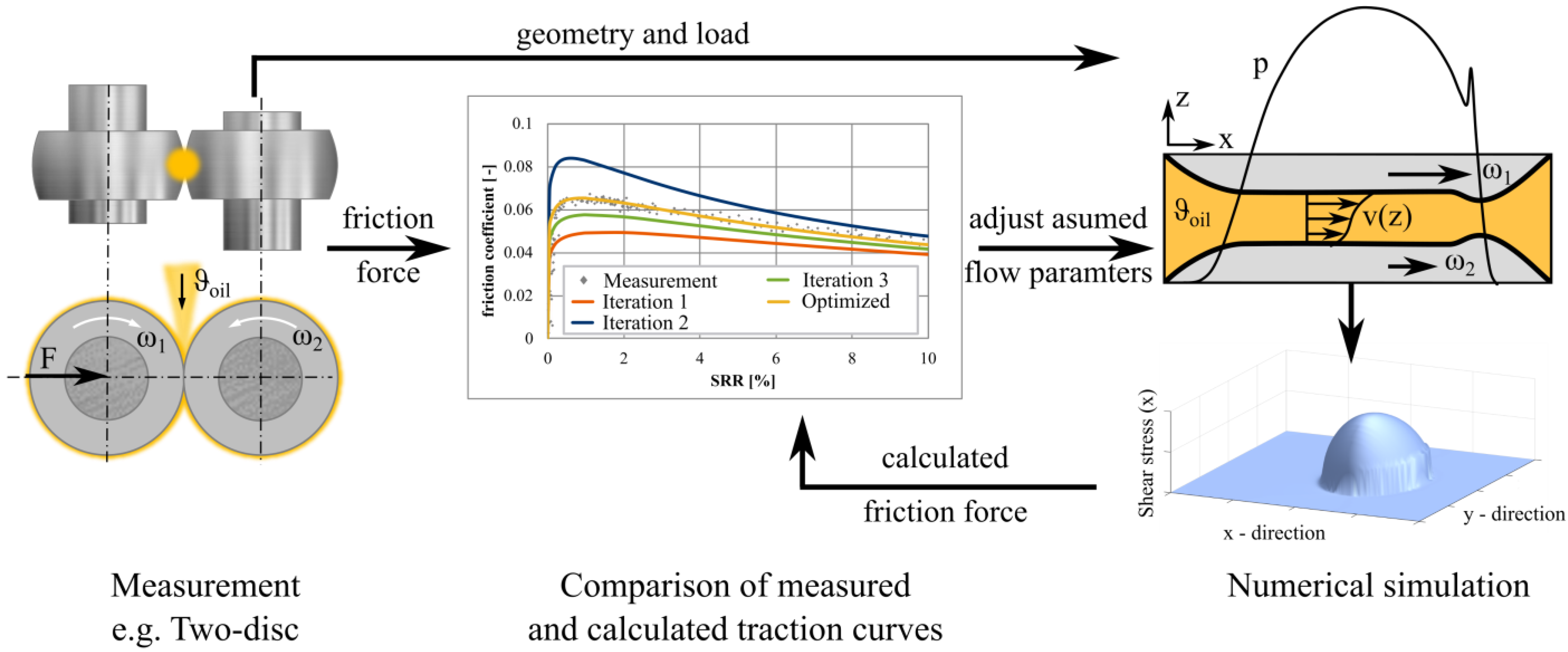
1.2.2. Option II—Traction Measurements
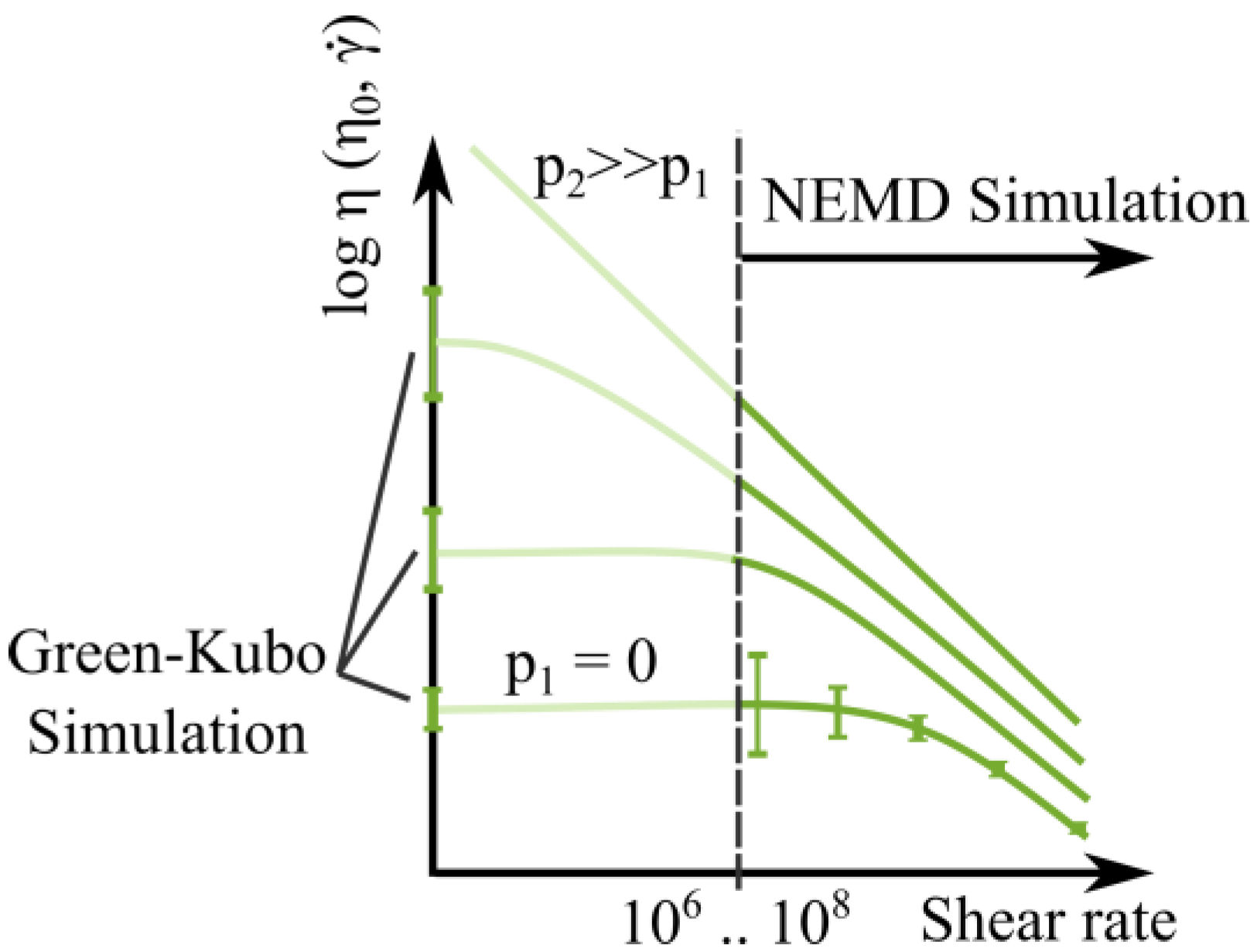
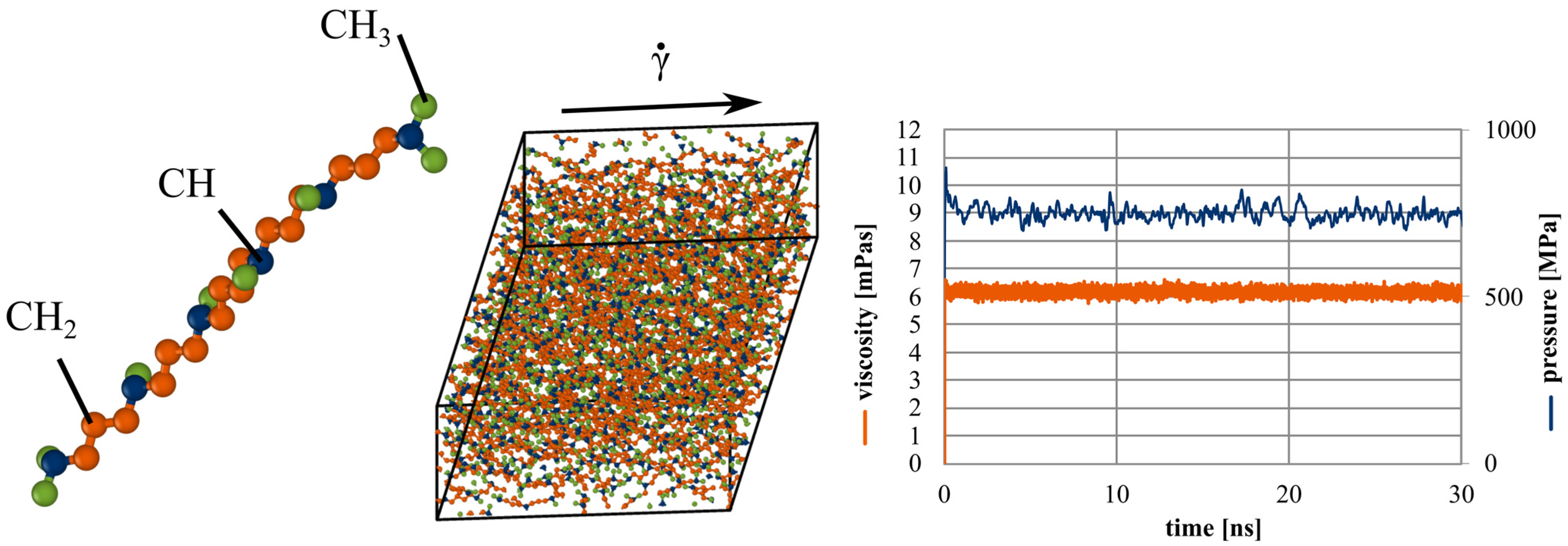
1.2.3. Option III—Molecular Dynamics Simulations
1.3. Limiting Shear Stress
1.4. Model Fluid Squalane as Object of Investigation
1.5. Conclusion and Aim of the Study
2. Materials and Methods
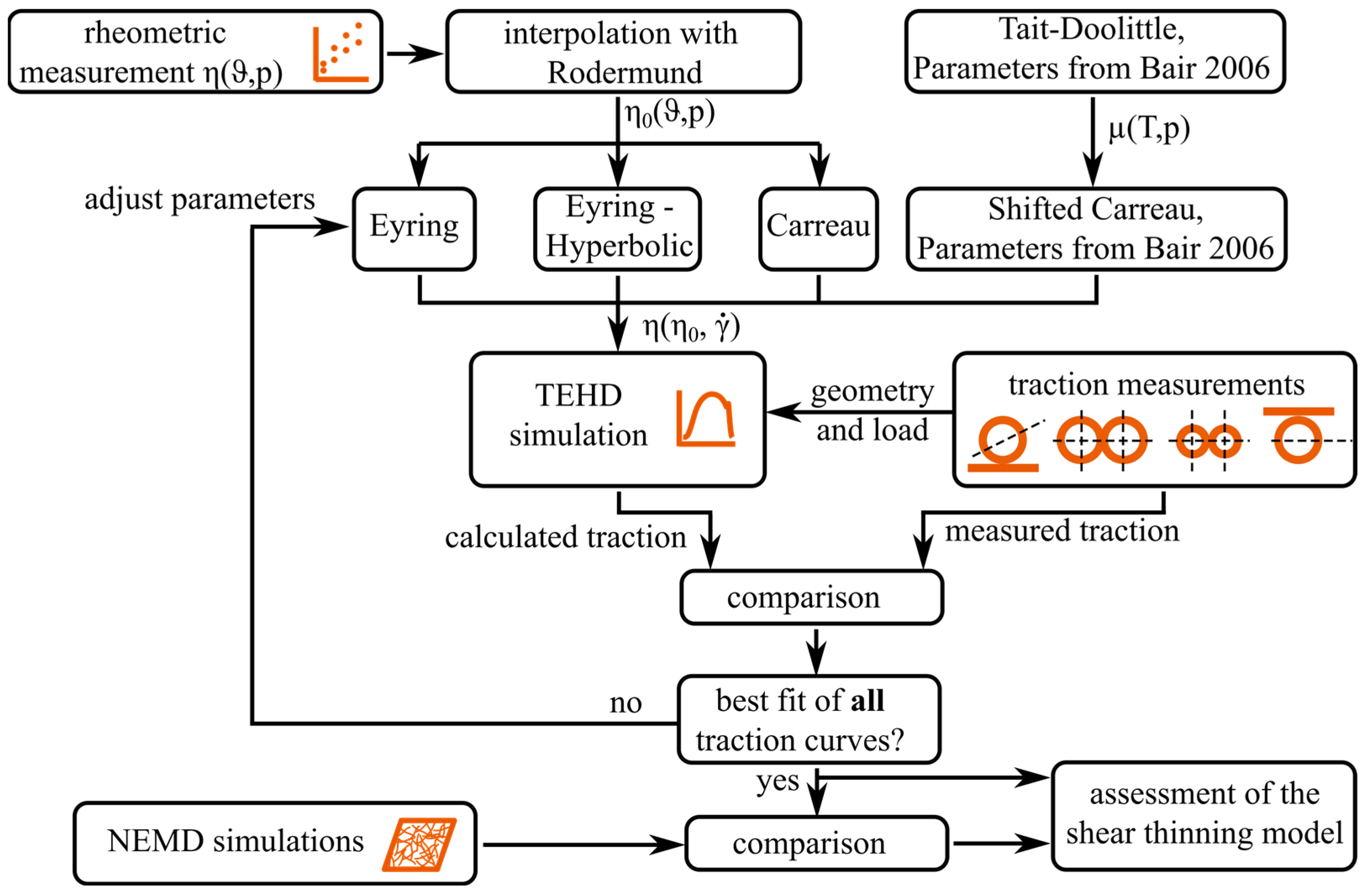
2.1. Fluid Modelling
2.2. Traction Measurements
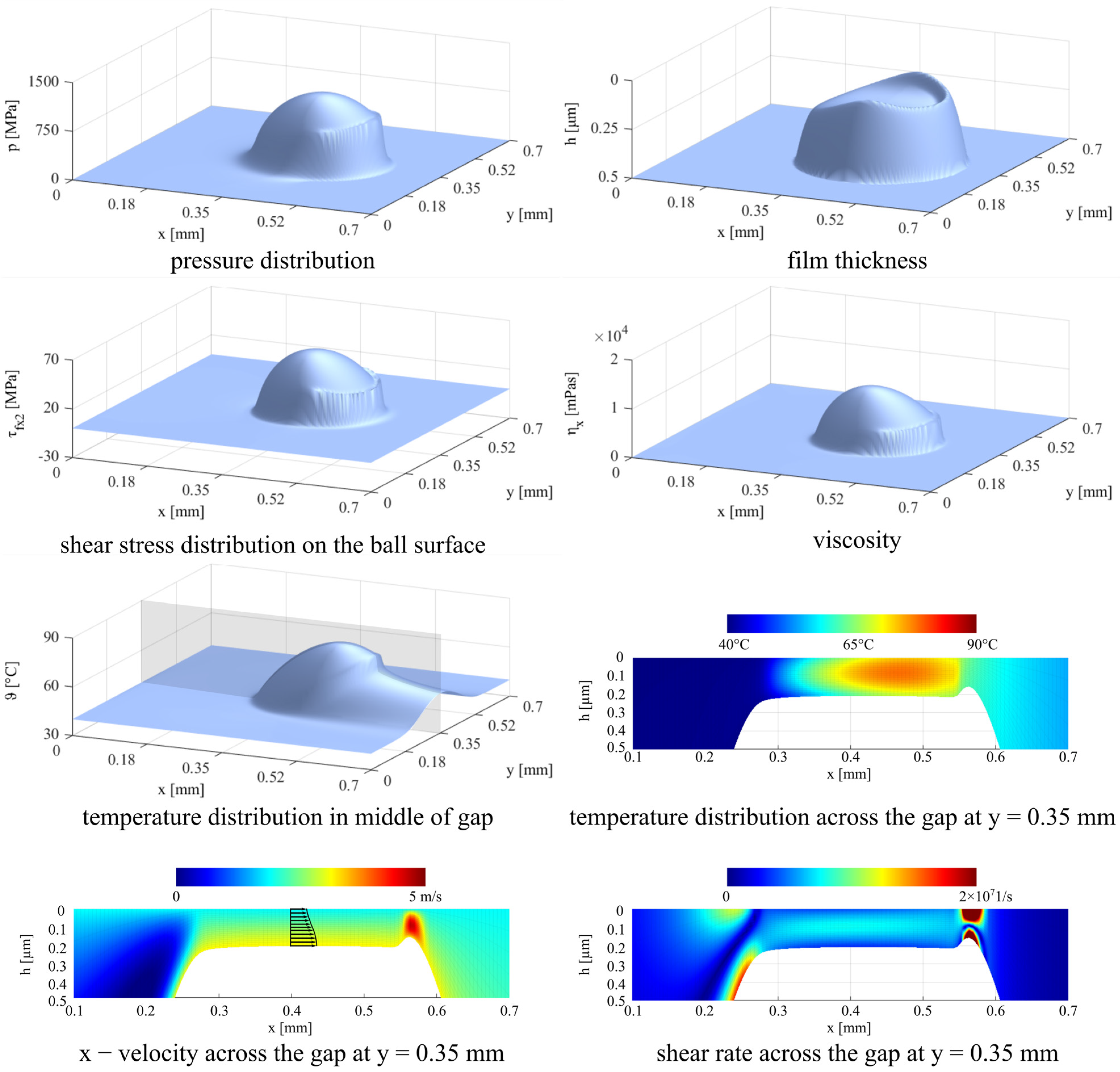
2.3. Iterative Optimisation Using TEHD Simulations
3. Results and Discussion
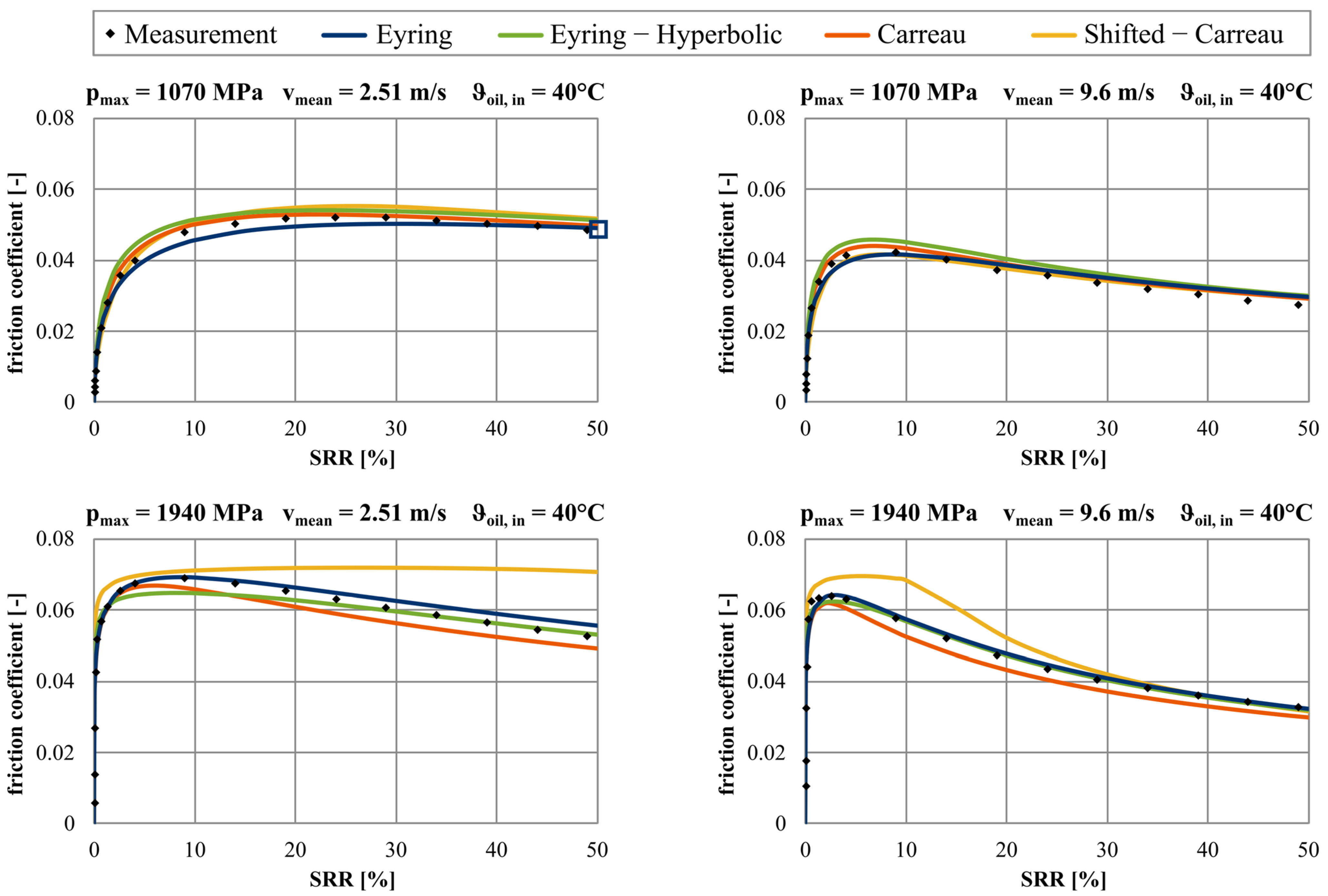
3.1. WAM11
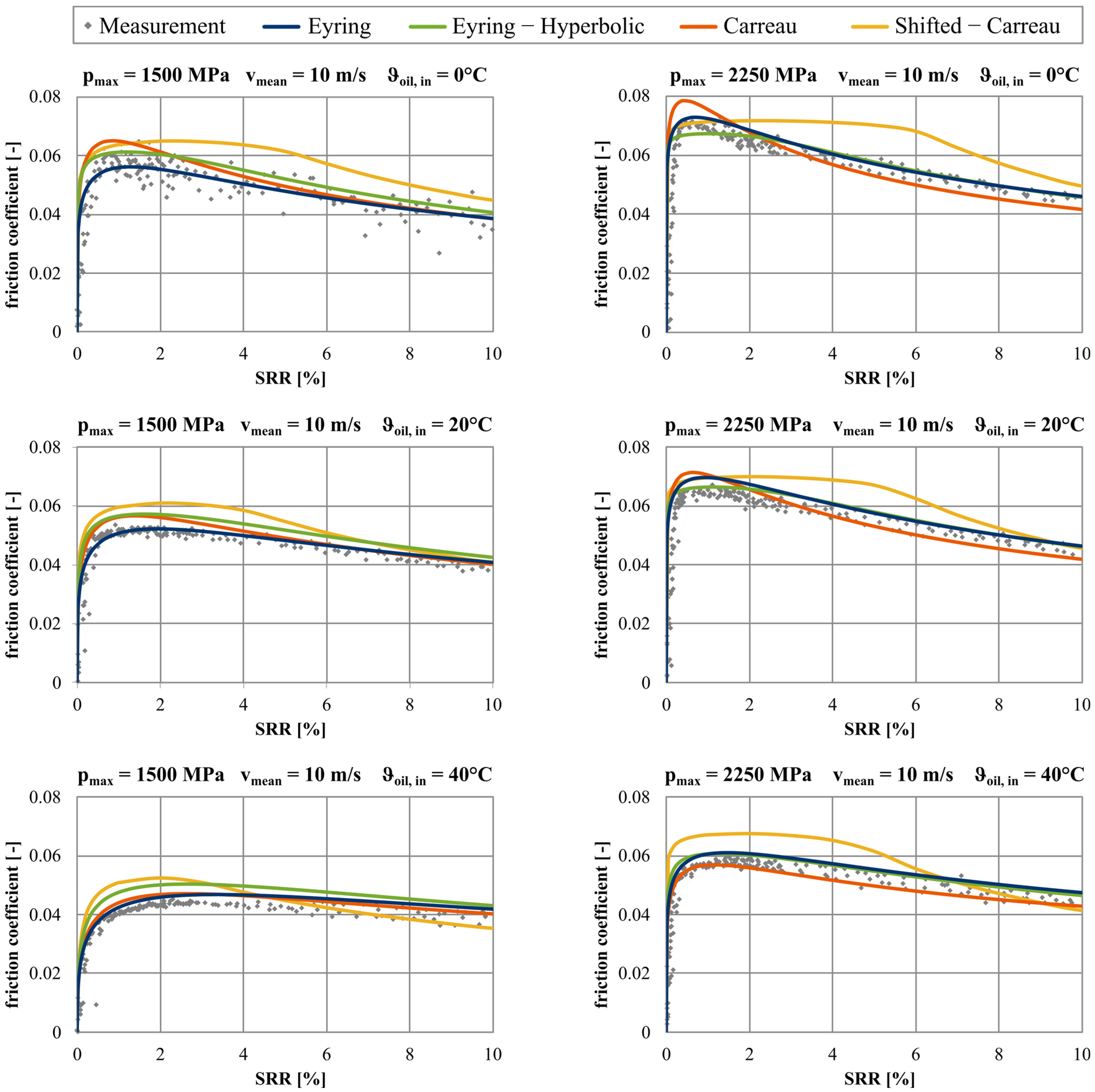
3.2. Large Two-Disc Machine
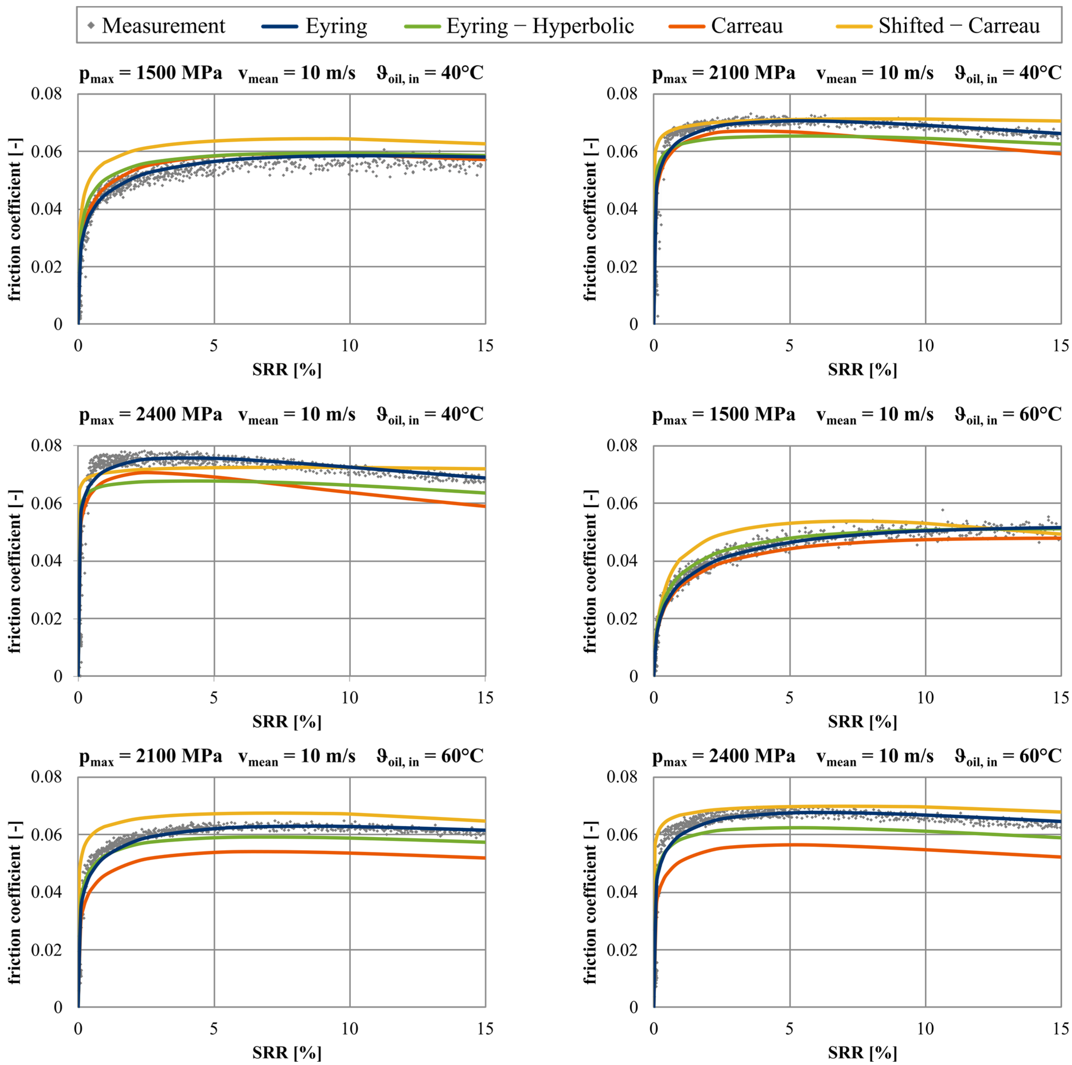
3.3. Small Two-Disc Machine
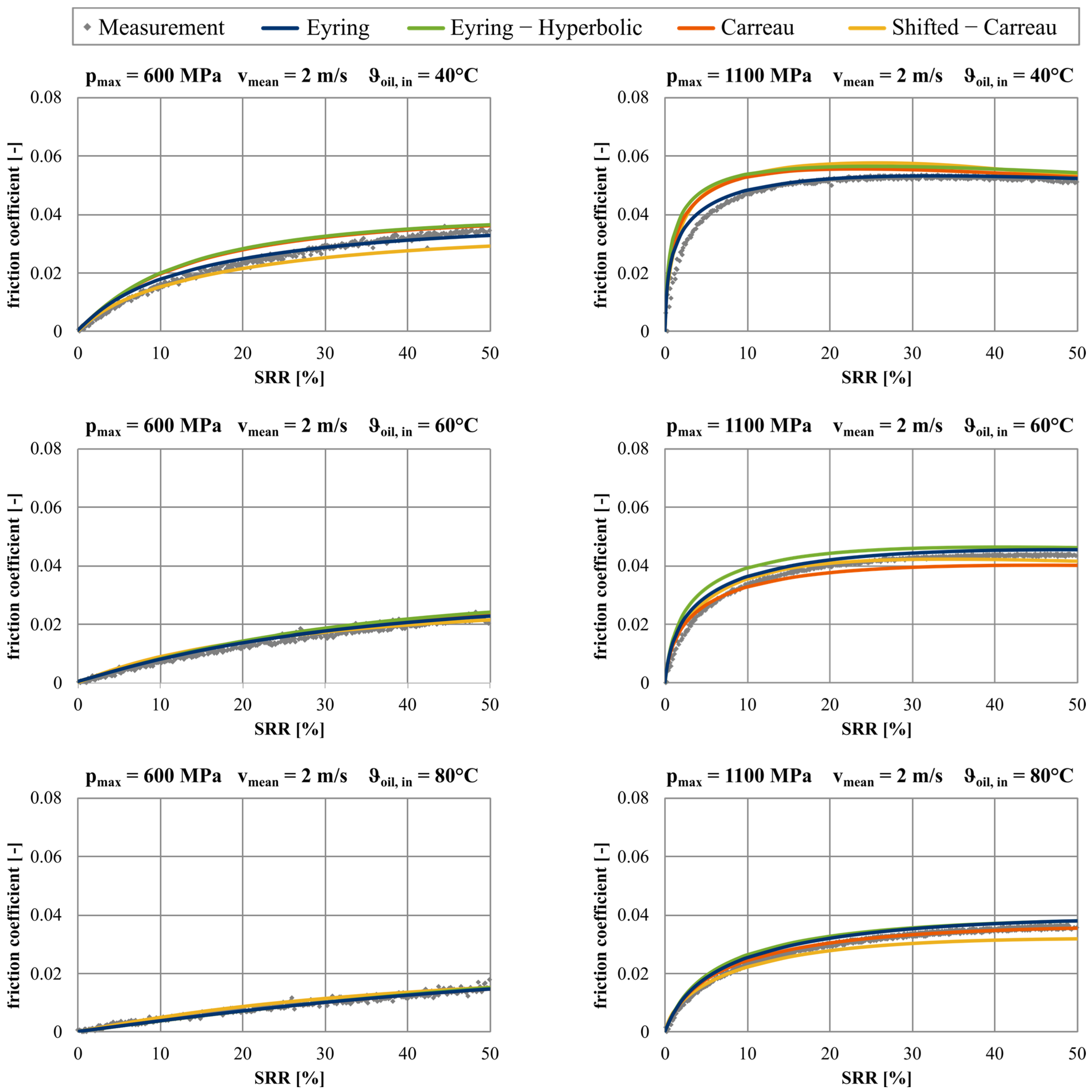
3.4. EHL2 Tribometer
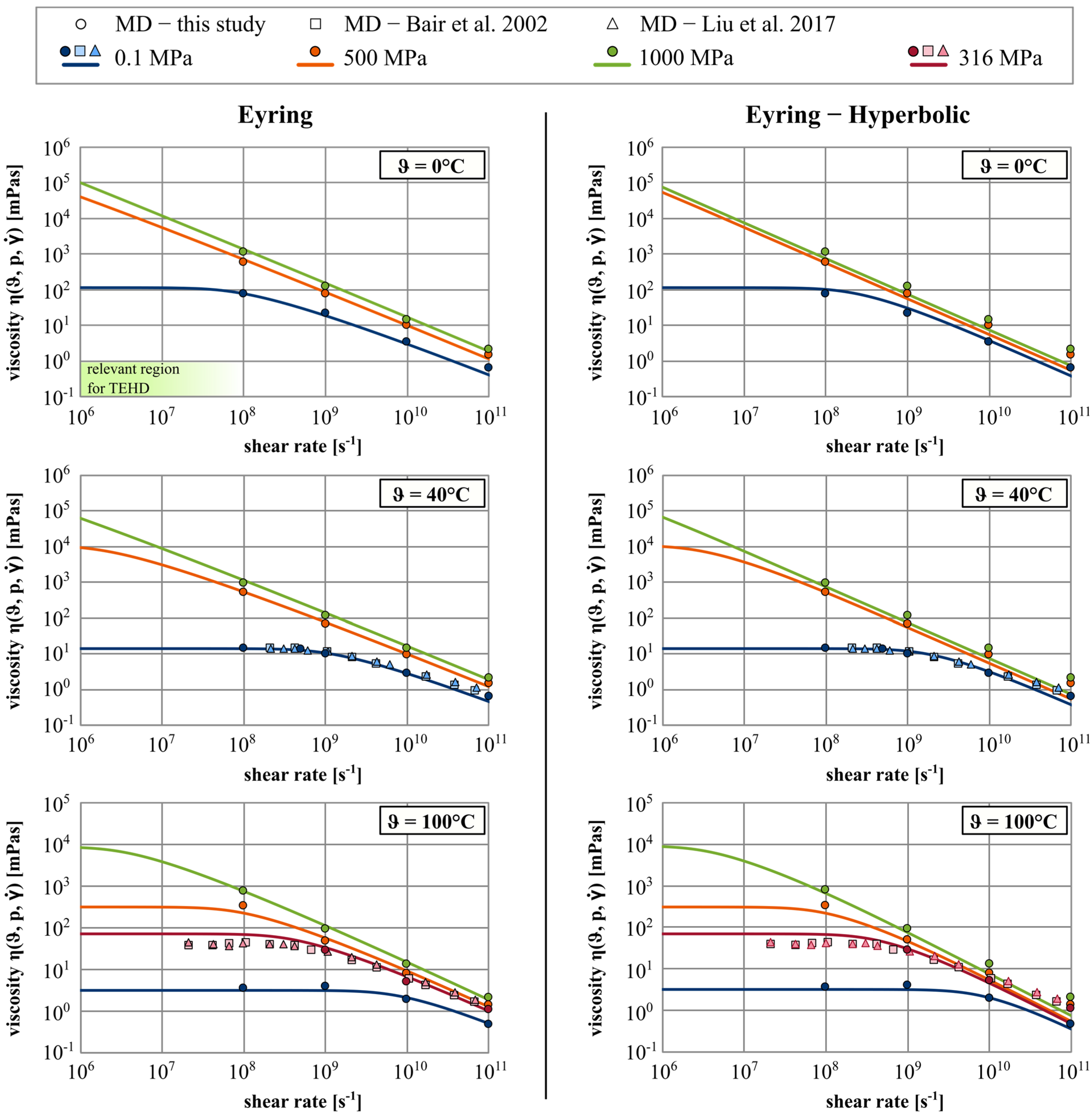
3.5. Comparison with Molecular Dynamics Simulations
4. Conclusions
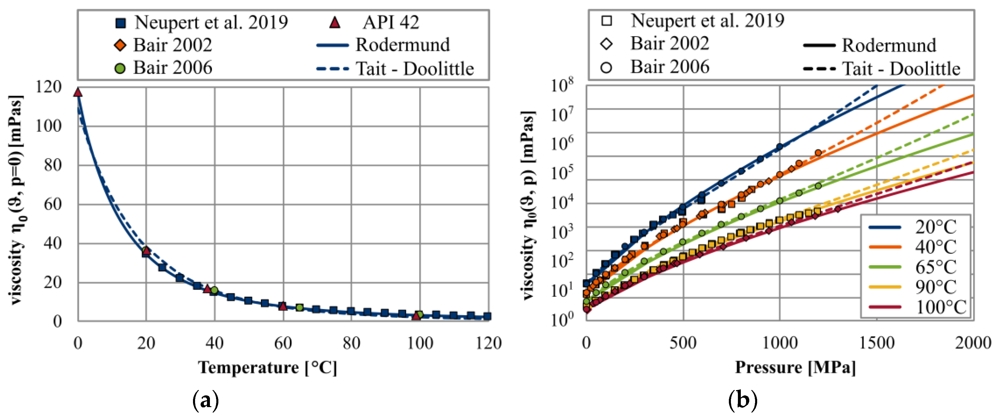
- For the modelling of low-shear viscosity, rheometric measurements from the literature were first collected, compared, and fitted with a degressive Rodermund model.
- In the measurement range, this modelling provides very similar values to the Tait–Doolittle equation used in the literature; however, in the extrapolated high-pressure range, the values are significantly lower due to the degressive curve.
- This modelling always leads to better agreements of the TEHD simulations with the traction curves than the degressive–progressive models.
- The general behaviour of the traction measurements is reproduced by all models.
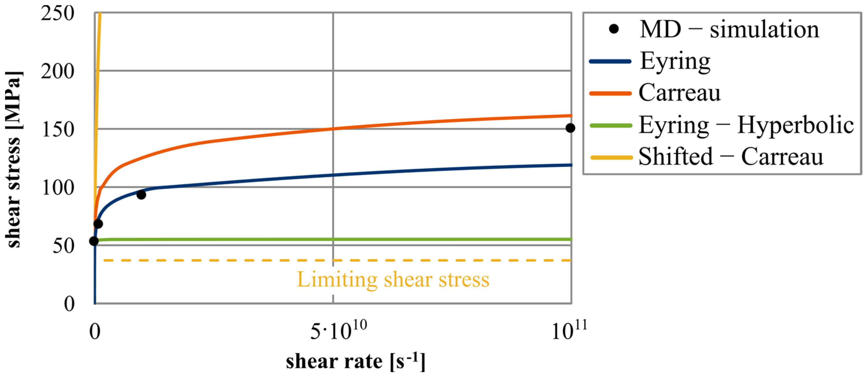
- The models with a limiting shear stress seem to limit the traction curve too much. Especially at high pressure, the traction behaviour is dominated by the limiting shear stress.
- The Carreau model only provides good agreement for certain cases. It can be assumed that this could be improved by variable parameters n and τc. Note: In subsequent calculations, no functional correlations for both parameters in terms of pressure and temperature could be found to improve the agreements.
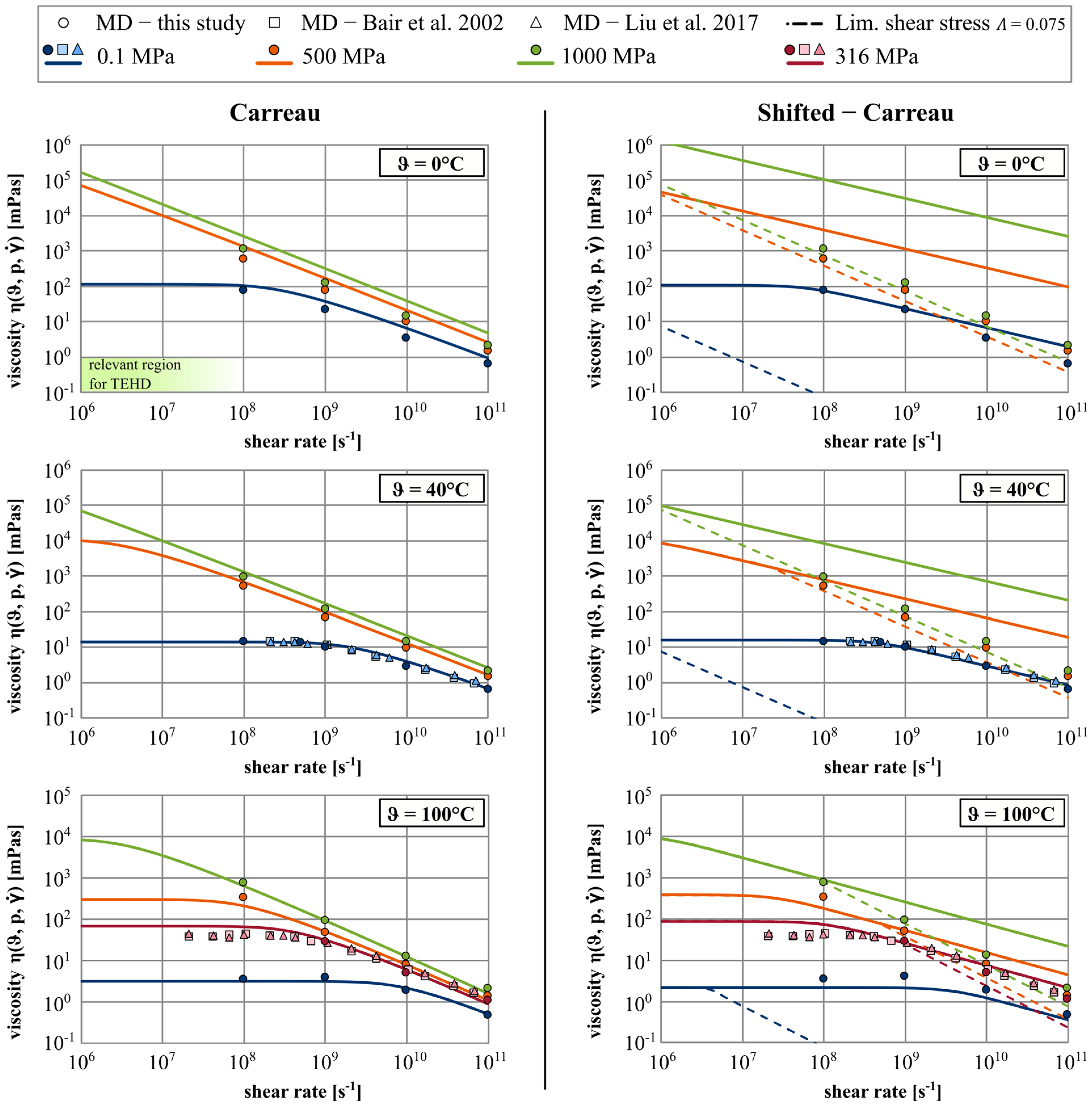
- It is possible to reproduce the NEMD simulation results from various sources with the described MD-model.
- The Eyring model again provides the best agreement when compared to the viscosity simulations for all temperatures and pressures.
- The Carreau model shows good agreement for high temperatures, but the modelled viscosity is too high for low temperatures. Variable parameters could help here.
- Analogous to the traction tests, a limiting shear stress acts too strongly. There is no evidence for a limiting shear stress from the SLLOD simulations carried out.
Author Contributions
Funding
Data Availability Statement
Conflicts of Interest
Abbreviation
| A | [°C] | Parameter of Rodermund equation |
| a | [Pa/K] | Parameter of critical shear stress equation |
| B | [°C] | Parameter of Rodermund equation |
| b | [-] | Parameter of critical shear stress equation |
| C | [°C] | Parameter of Rodermund equation |
| cp | [J/kg∙K] | Specific heat capacity |
| D | [-] | Parameter of Rodermund equation |
| E | [-] | Parameter of Rodermund equation |
| GR | [Pa] | Parameter of Shifted-Carreau equation |
| T | [K] | Temperature |
| TR | [K] | Reference Temperature |
| n | [-] | Exponent of Carreau equation |
| rc | [m] | Cutoff length of NEMD |
| t | [-] | Exponent of Eyring-Hyperbolic equation |
| p | [Pa] | Pressure |
| p0 | [Pa] | Parameter of Rodermund equation |
| plim | [Pa] | Transition pressure from exponential to linear limiting shear stress eq. |
| plim0 | [Pa] | Coefficient of limiting shear stress equation |
| v | [m/s] | Velocity |
| αp | [-] | Pressure–viscosity coefficient |
| β | [-] | Exponent of the linear limiting shear stress equation |
| βexp | [-] | Exponent of the exponential limiting shear stress equation |
| [s−1] | Shear rate | |
| ε | [J] | Bonding energy Lennard-Jones potential |
| η | [Pas] | Viscosity |
| η0 | [Pas] | Low-shear viscosity |
| ϑ | [°C] | Temperature |
| ϑ0 | [°C] | Reference temperature of τc0 |
| λ | [W/m∙K] | Thermal conductivity |
| μ | [Pas] | Low-shear viscosity for Shifted-Carreau equation |
| ρ | [kg/m3] | Density |
| σ | [m] | Distance where Lennard-Jones potential has a zero point |
| σxy | [Pa] | Shear stress in xy |
| τ | [Pa] | Shear stress within fluid |
| τc | [Pa] | Critical shear stress |
| τc0 | [Pa] | Critical shear stress at reference temperature |
| τlim | [Pa] | Limiting shear stress |
| τlim,0 | [Pa] | Limiting shear stress at ambient pressure |
| ω1,2 | [s−1] | Angular velocity |
| Λ | [-] | Gradient of limiting shear stress equation |
Appendix A. Structure and Parameters of the Used Squalane Molecule Based on ATB [53]

| Type | ε [kcal/mol] | σ [Å] |
|---|---|---|
| CH | 0.022679 | 5.01918 |
| CH2 | 0.09812 | 4.07038 |
| CH3 | 0.2073 | 3.7479 |
| # | Type | x [Å] | y [Å] | z [Å] | # | Type | x [Å] | y [Å] | z [Å] |
|---|---|---|---|---|---|---|---|---|---|
| 1 | CH3 | −13.424 | −2.309 | 0.541 | 16 | CH2 | 4.243 | −0.062 | 1.024 |
| 2 | CH | −12.610 | −1.039 | 0.686 | 17 | CH2 | 5.500 | −0.799 | 0.613 |
| 3 | CH2 | −11.398 | −1.085 | −0.234 | 18 | CH2 | 6.738 | −0.013 | 0.991 |
| 4 | CH2 | −10.337 | −0.079 | 0.160 | 19 | CH | 8.022 | −0.757 | 0.644 |
| 5 | CH2 | −9.136 | −0.168 | −0.758 | 20 | CH2 | 9.176 | 0.232 | 0.541 |
| 6 | CH | −8.034 | 0.807 | −0.364 | 21 | CH2 | 10.445 | −0.409 | 0.019 |
| 7 | CH2 | −6.720 | 0.393 | −1.015 | 22 | CH2 | 11.513 | 0.634 | −0.235 |
| 8 | CH2 | −5.524 | 1.078 | −0.388 | 23 | CH3 | −13.476 | 0.170 | 0.399 |
| 9 | CH2 | −4.232 | 0.581 | −1.001 | 24 | CH3 | −8.406 | 2.224 | −0.749 |
| 10 | CH | −3.004 | 1.206 | −0.350 | 25 | CH3 | −2.842 | 2.651 | −0.777 |
| 11 | CH2 | −1.764 | 0.394 | −0.699 | 26 | CH3 | 2.786 | −2.096 | 1.143 |
| 12 | CH2 | −0.592 | 0.714 | 0.204 | 27 | CH3 | 8.314 | −1.832 | 1.670 |
| 13 | CH2 | 0.594 | −0.176 | −0.105 | 28 | CH | 12.843 | 0.015 | −0.643 |
| 14 | CH2 | 1.775 | 0.163 | 0.780 | 29 | CH3 | 13.950 | 1.044 | −0.533 |
| 15 | CH | 2.977 | −0.734 | 0.510 | 30 | CH3 | 12.787 | −0.541 | −2.050 |
| # | UA 1 | UA 2 | # | UA 1 | UA 2 |
|---|---|---|---|---|---|
| 1 | 30 | 28 | 16 | 12 | 11 |
| 2 | 28 | 29 | 17 | 11 | 10 |
| 3 | 28 | 22 | 18 | 10 | 25 |
| 4 | 22 | 21 | 19 | 10 | 9 |
| 5 | 21 | 20 | 20 | 9 | 8 |
| 6 | 20 | 19 | 21 | 8 | 7 |
| 7 | 19 | 27 | 22 | 7 | 6 |
| 8 | 19 | 18 | 23 | 6 | 24 |
| 9 | 18 | 17 | 24 | 6 | 5 |
| 10 | 17 | 16 | 25 | 5 | 4 |
| 11 | 16 | 15 | 26 | 4 | 3 |
| 12 | 15 | 26 | 27 | 3 | 2 |
| 13 | 15 | 14 | 28 | 2 | 1 |
| 14 | 14 | 13 | 29 | 2 | 23 |
| 15 | 13 | 12 | |||
| Kbond [kcal/(mol·Å2) | r0 [Å] | ||||
| 299.844 | 1.52 | ||||
| # | Type | UA 1 | UA 2 | UA 3 | # | Type | UA 1 | UA 2 | UA 3 |
|---|---|---|---|---|---|---|---|---|---|
| 1 | 1 | 30 | 28 | 29 | 18 | 2 | 13 | 12 | 11 |
| 2 | 2 | 30 | 28 | 22 | 19 | 2 | 12 | 11 | 10 |
| 3 | 1 | 29 | 28 | 22 | 20 | 2 | 11 | 10 | 25 |
| 4 | 2 | 28 | 22 | 21 | 21 | 1 | 11 | 10 | 9 |
| 5 | 2 | 22 | 21 | 20 | 22 | 2 | 25 | 10 | 9 |
| 6 | 2 | 21 | 20 | 19 | 23 | 2 | 10 | 9 | 8 |
| 7 | 2 | 20 | 19 | 27 | 24 | 2 | 9 | 8 | 7 |
| 8 | 1 | 20 | 19 | 18 | 25 | 2 | 8 | 7 | 6 |
| 9 | 2 | 27 | 19 | 18 | 26 | 2 | 7 | 6 | 24 |
| 10 | 2 | 19 | 18 | 17 | 27 | 1 | 7 | 6 | 5 |
| 11 | 2 | 18 | 17 | 16 | 28 | 2 | 24 | 6 | 5 |
| 12 | 2 | 17 | 16 | 15 | 29 | 2 | 6 | 5 | 4 |
| 13 | 2 | 16 | 15 | 26 | 30 | 2 | 5 | 4 | 3 |
| 14 | 1 | 16 | 15 | 14 | 31 | 2 | 4 | 3 | 2 |
| 15 | 2 | 26 | 15 | 14 | 32 | 1 | 3 | 2 | 1 |
| 16 | 2 | 15 | 14 | 13 | 33 | 2 | 3 | 2 | 23 |
| 17 | 2 | 14 | 13 | 12 | 34 | 1 | 1 | 2 | 23 |
| Type | Kangle [kcal/(mol·rad2)] | φ0 [°] | |||||||
| 1 | 55.127 | 109.5 | |||||||
| 2 | 55.11 | 111 | |||||||
| # | Type | UA 1 | UA 2 | UA 3 | UA 4 | # | Type | UA 1 | UA 2 | UA 3 | UA 4 |
|---|---|---|---|---|---|---|---|---|---|---|---|
| 1 | 2 | 30 | 28 | 22 | 21 | 17 | 1 | 13 | 12 | 11 | 10 |
| 2 | 1 | 28 | 22 | 21 | 20 | 18 | 2 | 12 | 11 | 10 | 25 |
| 3 | 1 | 29 | 28 | 22 | 21 | 19 | 1 | 12 | 11 | 10 | 9 |
| 4 | 1 | 22 | 21 | 20 | 19 | 20 | 1 | 11 | 10 | 9 | 8 |
| 5 | 2 | 21 | 20 | 19 | 27 | 21 | 1 | 10 | 9 | 8 | 7 |
| 6 | 1 | 21 | 20 | 19 | 18 | 22 | 2 | 25 | 10 | 9 | 8 |
| 7 | 1 | 20 | 19 | 18 | 17 | 23 | 1 | 9 | 8 | 7 | 6 |
| 8 | 1 | 19 | 18 | 17 | 16 | 24 | 2 | 8 | 7 | 6 | 24 |
| 9 | 2 | 27 | 19 | 18 | 17 | 25 | 1 | 8 | 7 | 6 | 5 |
| 10 | 1 | 18 | 17 | 16 | 15 | 26 | 1 | 7 | 6 | 5 | 4 |
| 11 | 2 | 17 | 16 | 15 | 26 | 27 | 1 | 6 | 5 | 4 | 3 |
| 12 | 1 | 17 | 16 | 15 | 14 | 28 | 2 | 24 | 6 | 5 | 4 |
| 13 | 1 | 16 | 15 | 14 | 13 | 29 | 1 | 5 | 4 | 3 | 2 |
| 14 | 1 | 15 | 14 | 13 | 12 | 30 | 1 | 4 | 3 | 2 | 1 |
| 15 | 2 | 26 | 15 | 14 | 13 | 31 | 2 | 4 | 3 | 2 | 23 |
| 16 | 1 | 14 | 13 | 12 | 11 | ||||||
| Type | Kdihedral [kcal/(mol)] | d [-] | n [-] | ||||||||
| 1 | 1.415 | 1 | 3 | ||||||||
| 2 | 0 | 1 | 1 | Dummy for 1–4 interactions | |||||||
| # | UA 1 | UA 2 | UA 3 | UA 4 |
|---|---|---|---|---|
| 1 | 2 | 3 | 1 | 23 |
| 2 | 6 | 7 | 5 | 24 |
| 3 | 10 | 11 | 9 | 25 |
| 4 | 15 | 16 | 14 | 26 |
| 5 | 19 | 20 | 18 | 27 |
| 6 | 28 | 22 | 29 | 30 |
| Kimproper [kcal/(mol·rad2)] | χ0 [°] | |||
| 40.015 | 35.26 | |||
References
- Zhang, S.; Jacobs, G.; von Goeldel, S.; Vafaei, S.; König, F. Prediction of film thickness in starved EHL point contacts using two-phase flow CFD model. Tribol. Int. 2023, 178, 108103. [Google Scholar] [CrossRef]
- Hartinger, M.; Reddyhoff, T. CFD modeling compared to temperature and friction measurements of an EHL line contact. Tribol. Int. 2018, 126, 144–152. [Google Scholar] [CrossRef]
- Bartel, D. (Ed.) Simulation von Tribosystemen—Grundlagen und Anwendungen; Vieweg+Teubner: Wiesbaden, Germany, 2010. [Google Scholar] [CrossRef]
- Bobach, L.; Beilicke, B.; Bartel, D.; Deters, L. Thermal elastohydrodynamic simulation of involute spur gears incorporating mixed friction. Tribol. Int. 2012, 48, 191–206. [Google Scholar] [CrossRef]
- Bair, S. (Ed.) Chapter Eight—The Shear Dependence of Viscosity at Elevated Pressure. In High Pressure Rheology for Quantitative Elastohydrodynamics, 2nd ed.; Elsevier: Amsterdam, The Netherlands, 2019; pp. 223–257. [Google Scholar] [CrossRef]
- Powell, R.L. Rotational viscometry. In Rheological Measurement, 2nd ed.; Collyer, A.A., Clegg, D.W., Eds.; Springer: Dordrecht, The Netherlands, 1998. [Google Scholar] [CrossRef]
- Marin, G. Oscillatory rheometry. In Rheological Measurement, 2nd ed.; Collyer, A.A., Clegg, D.W., Eds.; Springer: Dordrecht, The Netherlands, 1998. [Google Scholar] [CrossRef]
- Bair, S. Reference liquids for quantitative elastohydrodynamics: Selection and rheological characterization. Tribol. Lett. 2006, 22, 197–206. [Google Scholar] [CrossRef]
- Bair, S.; Habchi, W. The Role of Fragility in Thermal Elastohydrodynamics. Tribol. Lett. 2023, 71, 24. [Google Scholar] [CrossRef]
- Spikes, H.; Zhang, J. History, Origins and Prediction of Elastohydrodynamic Friction. Tribol. Lett. 2014, 56, 1–25. [Google Scholar] [CrossRef]
- Bair, S.; Vergne, P.; Kumar, P.; Poll, G.; Krupka, I.; Hartl, M.; Habchi, W.; Larsson, R. Comment on “History, Origins and Prediction of Elastohydrodynamic Friction” by Spikes and Jie. Tribol. Lett. 2015, 58, 16. [Google Scholar] [CrossRef]
- Spikes, H.; Zhang, J. Reply to the Comment by Scott Bair, Philippe Vergne, Punit Kumar, Gerhard Poll, Ivan Krupka, Martin Hartl, Wassim Habchi, Roland Larson on “History, origins and prediction of elastohydrodynamic friction” by Spikes and Jie in tribology letters. Tribol. Lett. 2015, 58, 17. [Google Scholar] [CrossRef]
- Bair, S. Actual Eyring Models for Thixotropy and Shear-Thinning: Experimental Validation and Application to EHD. J. Tribol. 2004, 126, 728–732. [Google Scholar] [CrossRef]
- Zhang, J.; Spikes, H. Measurement of EHD Friction at Very High Contact Pressures. Tribol. Lett. 2020, 68, 42. [Google Scholar] [CrossRef]
- ASTM D4683-20; Standard Test Method for Measuring Viscosity of New and Used Engine Oils at High Shear Rate and High Temperature by Tapered Bearing Simulator Viscometer at 150 °C. ASTM: West Conshohocken, PA, USA, 2020. [CrossRef]
- Marx, N.; Ponjavic, A.; Taylor, R.I.; Spikes, H.A. Study of Permanent Shear Thinning of VM Polymer Solutions. Tribol. Lett. 2017, 65, 106. [Google Scholar] [CrossRef]
- Bair, S. The high pressure rheology of some simple model hydrocarbons. Proc. Inst. Mech. Eng. Part J J. Eng. Tr. 2002, 216, 139–149. [Google Scholar] [CrossRef]
- Jacobson, B.O. High-pressure chamber measurements. Proc. Inst. Mech. Eng. Part J J. Eng. Tr. 2006, 220, 199–206. [Google Scholar] [CrossRef]
- Björling, M.; Habchi, W.; Bair, S.; Larsson, R.; Marklund, P. Towards the true prediction of EHL friction. Tribol. Int. 2013, 66, 19–26, Erratum in Tribol. Int. 2019, 133, 297. [Google Scholar] [CrossRef]
- Liu, H. Traction Prediction in Rolling/Sliding EHL Contacts with Reference Fluids. Ph.D. Thesis, Gottfried Wilhelm Leibniz Universität, Hannover, Germany, 2020. [Google Scholar]
- Ndiaye, S.-N.; Martinie, L.; Philippon, D.; Devaux, N.; Vergne, P. A Quantitative Friction-Based Approach of the Limiting Shear Stress Pressure and Temperature Dependence. Tribol. Lett. 2017, 65, 149. [Google Scholar] [CrossRef]
- Neupert, T.; Brouwer, L.; Slabka, I.; Terwey, T. Tribological Fluid Models II. Final Report, FVV Project No. 1277; Research Association for Internal Combustion Engines (FVV): Frankfurt, Germany, 2019. [Google Scholar]
- Bair, S.; McCabe, C.; Cummings, P.T. Comparison of Nonequilibrium Molecular Dynamics with Experimental Measurements in the Nonlinear Shear-Thinning Regime. Phys. Rev. Lett. 2002, 88, 058302-1–058302-4. [Google Scholar] [CrossRef] [PubMed]
- Liu, P.; Lu, J.; Yu, H.; Ren, N.; Lockwood, F.E.; Wang, Q.J. Lubricant shear thinning behavior correlated with variation of radius of gyration via molecular dynamics simulations. J. Chem. Phys. 2017, 147, 084904. [Google Scholar] [CrossRef] [PubMed]
- Jadhao, V.; Robbins, M.O. Probing large viscosities in glassformers with nonequilibrium simulations. Proc. Natl. Acad. Sci. USA 2017, 114, 7952–7957. [Google Scholar] [CrossRef] [PubMed]
- Panwar, P.; Michael, P.; Devlin, M.; Martini, A. Critical Shear Rate of Polymer-Enhanced Hydraulic Fluids. Lubricants 2020, 8, 102. [Google Scholar] [CrossRef]
- Mathas, D.; Holweger, W.; Wolf, M.; Bohnert, C.; Bakolas, V.; Procelewska, J.; Wang, L.; Bair, S.; Skylaris, C.-K. Evaluation of Methods for Viscosity Simulations of Lubricants at Different Temperatures and Pressures: A Case Study on PAO-2. Tribol. Trans. 2021, 64, 1138–1148. [Google Scholar] [CrossRef]
- Ewen, J.P.; Spikes, H.A.; Dini, D. Contributions of Molecular Dynamics Simulations to Elastohydrodynamic Lubrication. Tribol. Lett. 2021, 69, 24. [Google Scholar] [CrossRef]
- Evans, D.J.; Holian, B.L. The Nose-Hoover thermostat. J. Chem. Phys. 1985, 83, 4069. [Google Scholar] [CrossRef]
- Evans, D.J.; Morriss, G.P. Nonlinear-response theory for steady planar Couette flow. Phys. Rev. A 1984, 30, 1528–1530. [Google Scholar] [CrossRef]
- Ewen, J.P.; Gattinoni, C.; Zhang, J.; Heyes, D.M.; Spikes, H.A.; Dini, D. On the effect of confined fluid molecular structure on nonequilibrium phase behaviour and friction. Phys. Chem. Chem. Phys. 2017, 19, 17883–17894. [Google Scholar] [CrossRef]
- Cui, S.T.; Cummings, P.T.; Cochran, H.D. The Calculation of Viscosity of Liquid n Decane and n-Hexadecane by the Green-Kubo Method. Mol. Phys. 1998, 93, 117–122. [Google Scholar] [CrossRef]
- Mondello, M.; Grest, G.S. Viscosity calculations of n-alkanes by equilibrium molecular dynamics. J. Chem. Phys. 1997, 106, 9327–9336. [Google Scholar] [CrossRef]
- Ewen, J.P.; Gattinoni, C.; Thakkar, F.M.; Morgan, N.; Spikes, H.A.; Dini, D. A Comparison of Classical Force-Fields for Molecular Dynamics Simulations of Lubricants. Materials 2016, 9, 651. [Google Scholar] [CrossRef]
- Zhang, Y.; Otani, A.; Maginn, E.J. Reliable Viscosity Calculation from Equilibrium Molecular Dynamics Simulations: A Time Decomposition Method. J. Chem. Theory Comput. 2015, 11, 3537–3546. [Google Scholar] [CrossRef]
- Bair, S.; Winer, W.O. The high shear stress rheology of liquid lubricants at pressures of 2 to 200 MPa. J. Tribol. 1990, 112, 246–252. [Google Scholar] [CrossRef]
- Bair, S.; Winer, W.O. The high pressure high shear stress rheology of liquid lubricants. J. Tribol. 1992, 114, 1–9. [Google Scholar] [CrossRef]
- Bair, S.; McCabe, C. A study of mechanical shear bands in liquids at high pressure. Tribol. Int. 2004, 37, 783–789. [Google Scholar] [CrossRef]
- Bair, S.; McCabe, C.; Cummings, T.P. Calculation of viscous EHL traction for squalane using molecular simulation and rheometry. Tribol. Lett. 2002, 13, 251–254. [Google Scholar] [CrossRef]
- Beilicke, R.; Bobach, L.; Bartel, B. Transient thermal elastohydrodynamic simulation of a DLC-coated helical gear pair considering limiting shear stress behavior of the lubricant. Tribol. Int. 2016, 97, 136–150. [Google Scholar] [CrossRef]
- Dixon, J.A.; Webb, W.; Steele, W.A. Properties of Hydrocarbons of High-Molecular Weight Synthesized by Research Project 42 of the American Petroleum Institute; Pennsylvania State University: Pennsylvania, PA, USA, 1962. [Google Scholar]
- Bair, S.; Yamaguchi, T.; Brouwer, L.; Schwarze, H.; Vergne, P.; Poll, G. Oscillatory and Steady Shear Viscosity of Liquid Lubricants: The Cox-Merz Rule, Superposition, and Application to EHL Friction. Tribol. Int. 2014, 79, 126–131. [Google Scholar] [CrossRef]
- Bair, S.; Andersson, O.; Qureshi, F.S.; Schirru, M.M. New EHL Modeling Data for the Reference Liquids Squalane and Squalane Plus Polyisoprene. Tribol. Trans. 2018, 61, 247–255. [Google Scholar] [CrossRef]
- Rodermund, H. Beitrag zur Elastohydrodynamischen Schmierung von Evolventenzahnrädern. Ph.D. Thesis, TU Clausthal, Clausthal, Germany, 1975. [Google Scholar]
- Eyring, H. Viscosity, Plasticity and Diffusion as Examples of Reaction Rates. J. Chem. Phys. 1936, 4, 283–291. [Google Scholar] [CrossRef]
- Wolff, R.; Kubo, A. A Generalized Non-Newtonian Fluid Model Incorporated into Elastohydrodynamic Lubrication. J. Tribol. 1996, 118, 74–82. [Google Scholar] [CrossRef]
- Bair, S.; Qureshi, F. The Generalized Newtonian Fluid Model and Elastohydrodynamic Film Thickness. J. Tribol. 2003, 125, 70–75. [Google Scholar] [CrossRef]
- Johnson, K.L.; Tevaarwerk, J.L.; Tabor, D. Shear behaviour of elastohydrodynamic oil films. Proc. R. Soc. A Math. Phys. Eng. Sci. 1977, 356, 215–236. [Google Scholar] [CrossRef]
- Bobach, L.; Bartel, D.; Beilicke, R.; Mayer, J.; Michaelis, K.; Stahl, K.; Bachmann, S.; Schnagl, J.; Ziegele, H. Reduction in EHL Friction by a DLC Coating. Tribol. Lett. 2015, 60, 17. [Google Scholar] [CrossRef]
- Bobach, L.; Beilicke, B.; Bartel, D. Transient thermal elastohydrodynamic simulation of a spiral bevel gear pair with an octoidal tooth profile under mixed friction conditions. Tribol. Int. 2020, 143, 106020. [Google Scholar] [CrossRef]
- Plimpton, S. Fast Parallel Algorithms for Short-Range Molecular Dynamics. J. Comput. Phys. 1995, 117, 1–19. [Google Scholar] [CrossRef]
- Malde, A.K.; Zuo, L.; Breeze, M.; Stroet, M.; Poger, D.; Nair, P.C.; Oostenbrink, C.; Mark, A.E. An Automated force field Topology Builder (ATB) and repository: Version 1.0. J. Chem. Theory Comput. 2011, 7, 4026–4037. [Google Scholar] [CrossRef] [PubMed]
- Schmid, N.; Eichenberger, A.P.; Choutko, A.; Riniker, S.; Winger, M.; Mark, A.E.; van Gunsteren, W.F. Definition and testing of the GROMOS force-field versions 54A7 and 54B7. Eur. Biophys. J. 2011, 40, 843–856. [Google Scholar] [CrossRef] [PubMed]
- Bair, S. Viscous heating in compressed liquid films. Tribol. Lett. 2020, 68, 7. [Google Scholar] [CrossRef]


| Model | Equation | Ref. | Used Parameters for Squalane | Limiting Shear Stress | |
|---|---|---|---|---|---|
| Eyring | (3) | [45] | No | ||
| (4) | |||||
| Eyring- Hyperbolic | (5) | [22,46] | Yes | ||
| (6) | |||||
| Carreau | (7) | [47] | No | ||
| Shifted- Carreau | (8) | [8] | Yes | ||
| (9) | [19,39] |
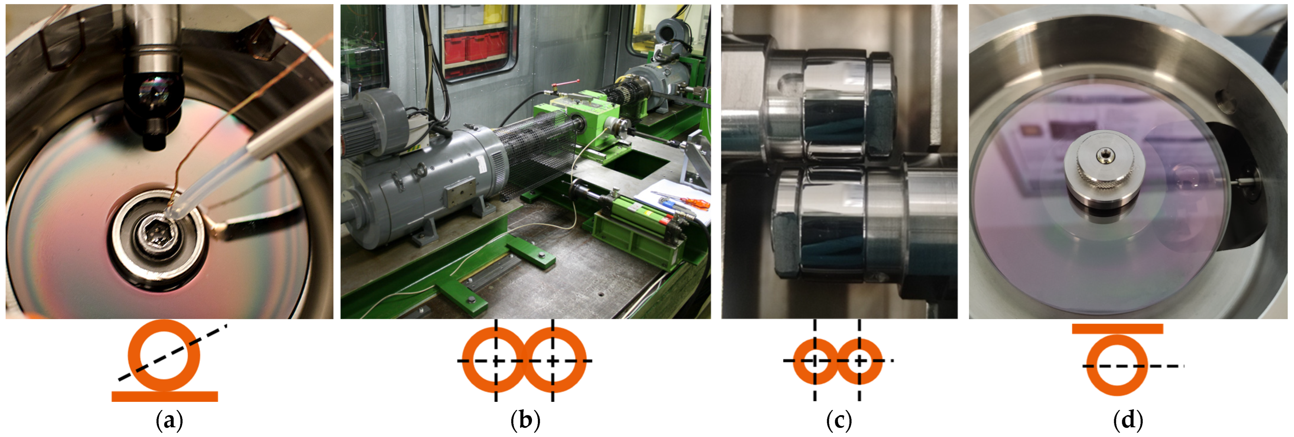
| WAM11 (Data from [19]) | Large Two-Disc Machine (Data from [22]) | Small Two-Disc Machine (Own Measurements) | EHL2 Tribometer (Own Measurements) | |
|---|---|---|---|---|
 |  |  |  | |
| Body 1 | ball | disc | disc | ball |
| Dimensions of body 1 | Ø 20.64 mm | Ø 120 mm crowning: R50 mm | Ø 20.4 mm crowning: R100 mm | Ø 19.05 mm |
| Body 2 | disc | disc | disc | disc |
| Dimensions of body 2 | raceway Ø 40 mm | Ø 120 mm cylindrical | Ø 20.4 mm crowning: R100 mm | raceway Ø 80 mm |
| Material | AISI52100 (100Cr6) | AISI52100 (100Cr6) | AISI52100 (100Cr6) | AISI52100 (100Cr6) |
| Roughness | ball: Rq = 25 nm disc: Rq = 35 nm comb.: Rq = 43 nm | body 1: Ra = 63 nm body 2: Ra = 26 nm comb.: Ra = 68 nm | Ra1,2 < 20 nm | Ra1,2 < 20 nm |
| Applied force | 50 N, 300 N | 1180 N, 1920 N 3750 N, 6500 N | 97 N, 230 N, 396 N, 629 N, 938 N, 1333 N | 8 N, 27 N, 50 N |
| Max. Hertzian Pressure | 1070 MPa, 1940 MPa | 1275 MPa, 1500 MPa 1875 MPa, 2250 MPa | 1200 MPa, 1500 MPa 1800 MPa, 2100 MPa 2400 MPa, 2700 MPa | 600 MPa, 900 MPa 1100 MPa |
| Oil feed temperature | 40 °C | 0 °C, 20 °C, 40 °C | 40 °C, 60 °C | 40 °C, 60 °C, 80 °C |
| Mean velocity | 0.34 m/s … 9.6 m/s 2.51 m/s, 9.6 m/s | 5 m/s, 10 m/s, 15 m/s | 5 m/s | 2 m/s, 3 m/s |
| SRR | 0.2% … 49% | −15 … 15% | −10 … 10% | −50 … 50% |
Disclaimer/Publisher’s Note: The statements, opinions and data contained in all publications are solely those of the individual author(s) and contributor(s) and not of MDPI and/or the editor(s). MDPI and/or the editor(s) disclaim responsibility for any injury to people or property resulting from any ideas, methods, instructions or products referred to in the content. |
© 2023 by the authors. Licensee MDPI, Basel, Switzerland. This article is an open access article distributed under the terms and conditions of the Creative Commons Attribution (CC BY) license (https://creativecommons.org/licenses/by/4.0/).
Share and Cite
Neupert, T.; Bartel, D. Evaluation of Various Shear-Thinning Models for Squalane Using Traction Measurements, TEHD and NEMD Simulations. Lubricants 2023, 11, 178. https://doi.org/10.3390/lubricants11040178
Neupert T, Bartel D. Evaluation of Various Shear-Thinning Models for Squalane Using Traction Measurements, TEHD and NEMD Simulations. Lubricants. 2023; 11(4):178. https://doi.org/10.3390/lubricants11040178
Chicago/Turabian StyleNeupert, Thomas, and Dirk Bartel. 2023. "Evaluation of Various Shear-Thinning Models for Squalane Using Traction Measurements, TEHD and NEMD Simulations" Lubricants 11, no. 4: 178. https://doi.org/10.3390/lubricants11040178
APA StyleNeupert, T., & Bartel, D. (2023). Evaluation of Various Shear-Thinning Models for Squalane Using Traction Measurements, TEHD and NEMD Simulations. Lubricants, 11(4), 178. https://doi.org/10.3390/lubricants11040178