Physical Analysis of Thermophoresis and Variable Density Effects on Heat Transfer Assessment along a Porous Stretching Sheet and Their Applications in Nanofluid Lubrication


Abstract
1. Introduction and Literature Review
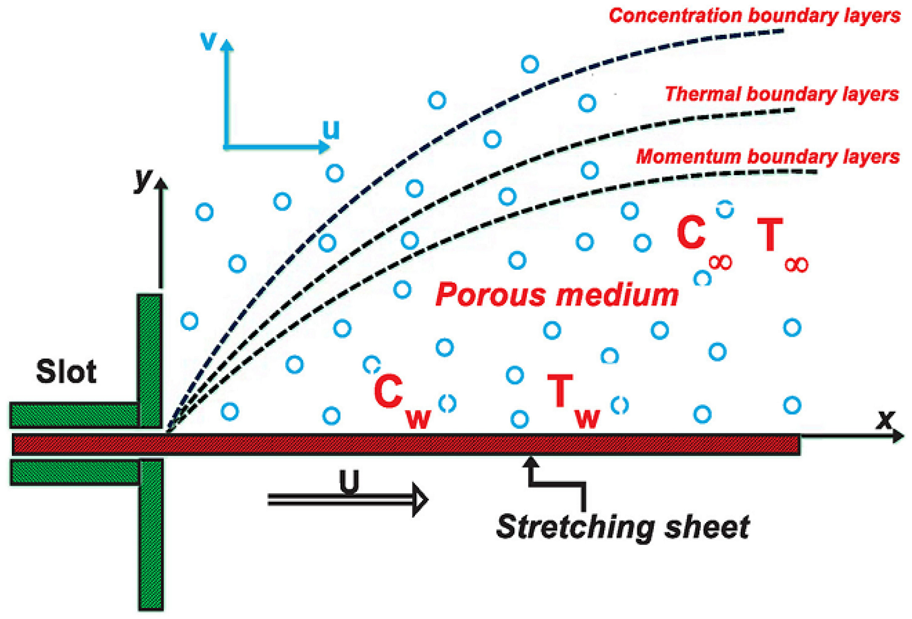
2. The Flow Geometry and Mathematical Formulation
3. Stream Functions and Similarity Variables
4. Computational Scheme and Solution Methodology
5. Matrix Form of Vector Equations
6. Quantitative and Physical Reasoning
7. Conclusions
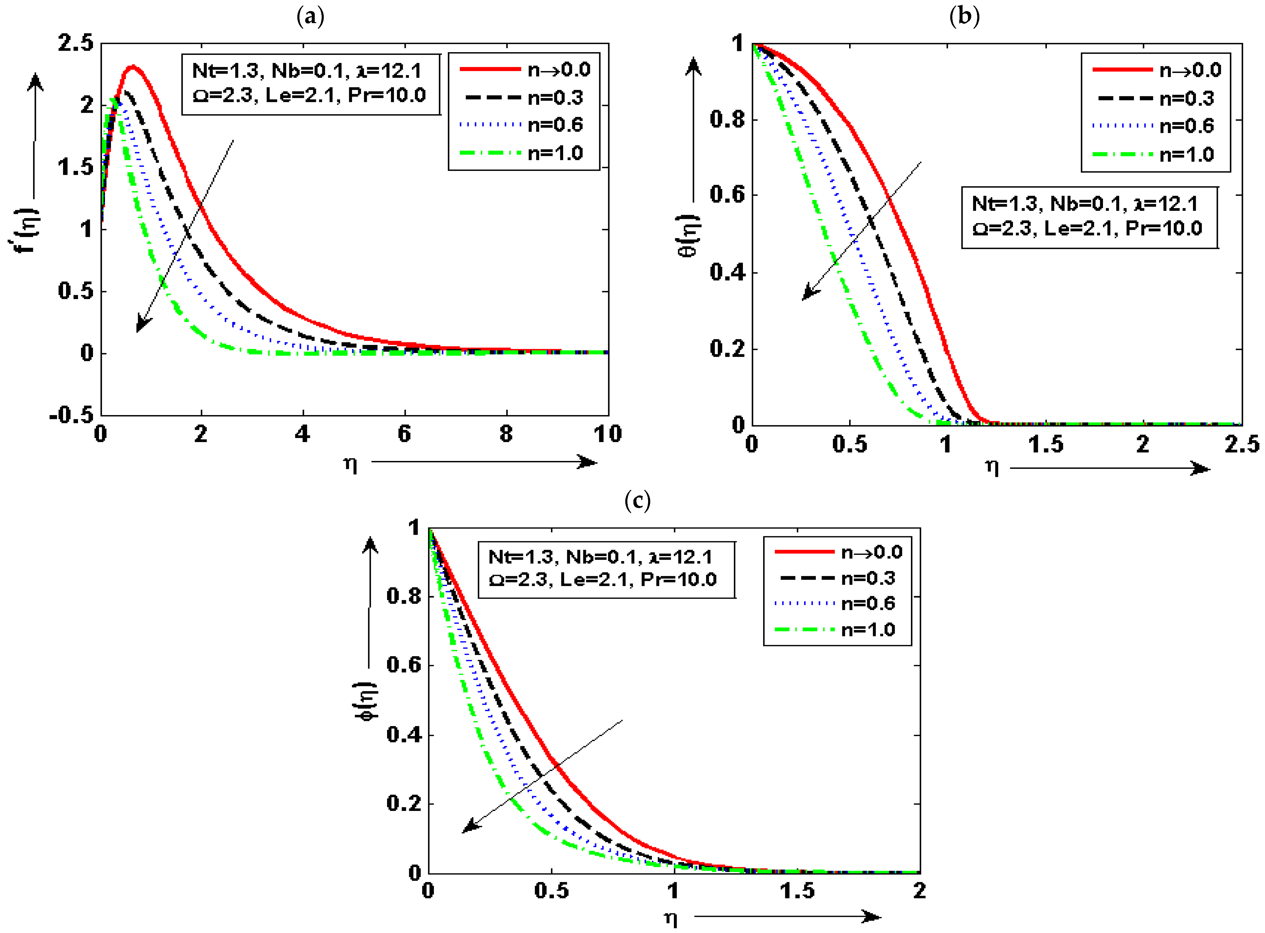
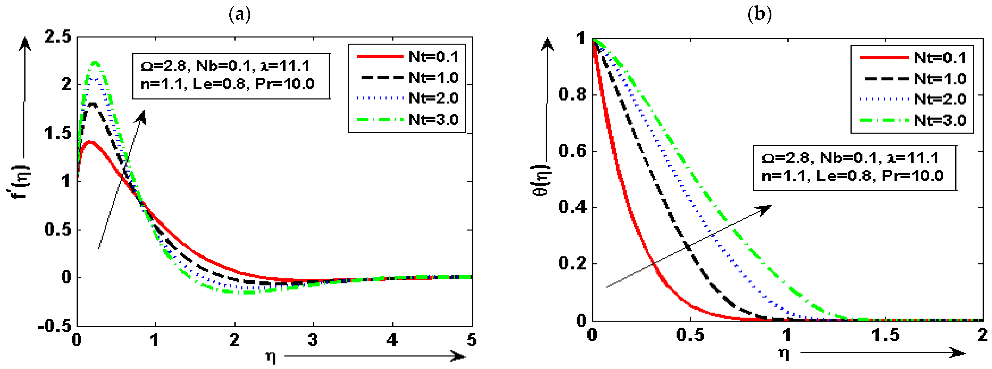
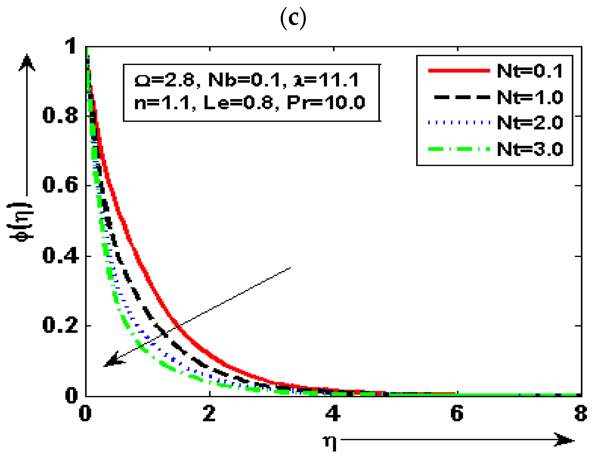
- The velocity plot is enhanced for minimum quantity of and reduced for maximum. The fluid concentration plot is increased for minimum quantity of and reduced for maximum;
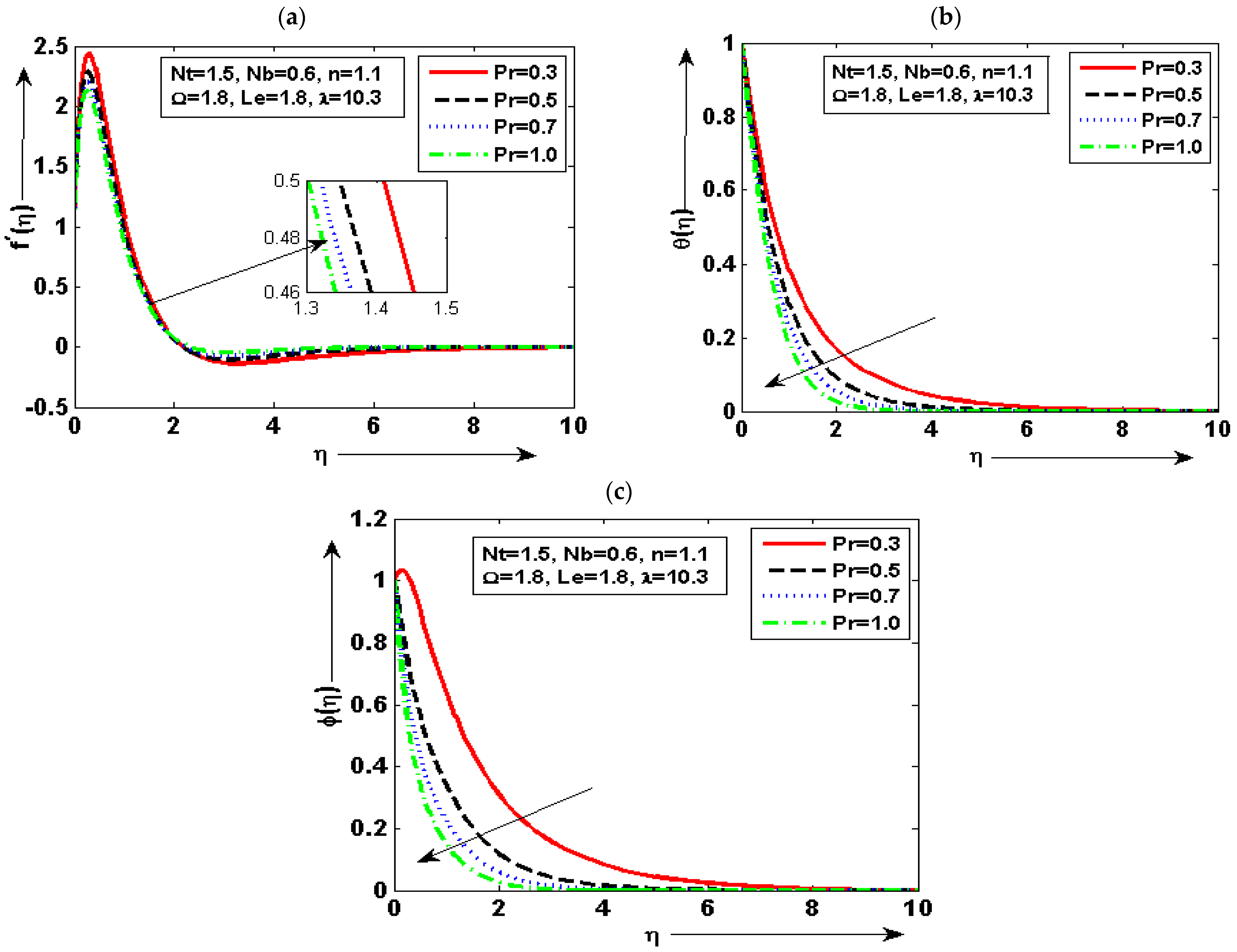
- The temperature graph is at a minimum by higher but increased by decreasing . It is deduced that of fluid is decreased with the increase of. The prominent variation in every plot is noted for diverse choices of density number;
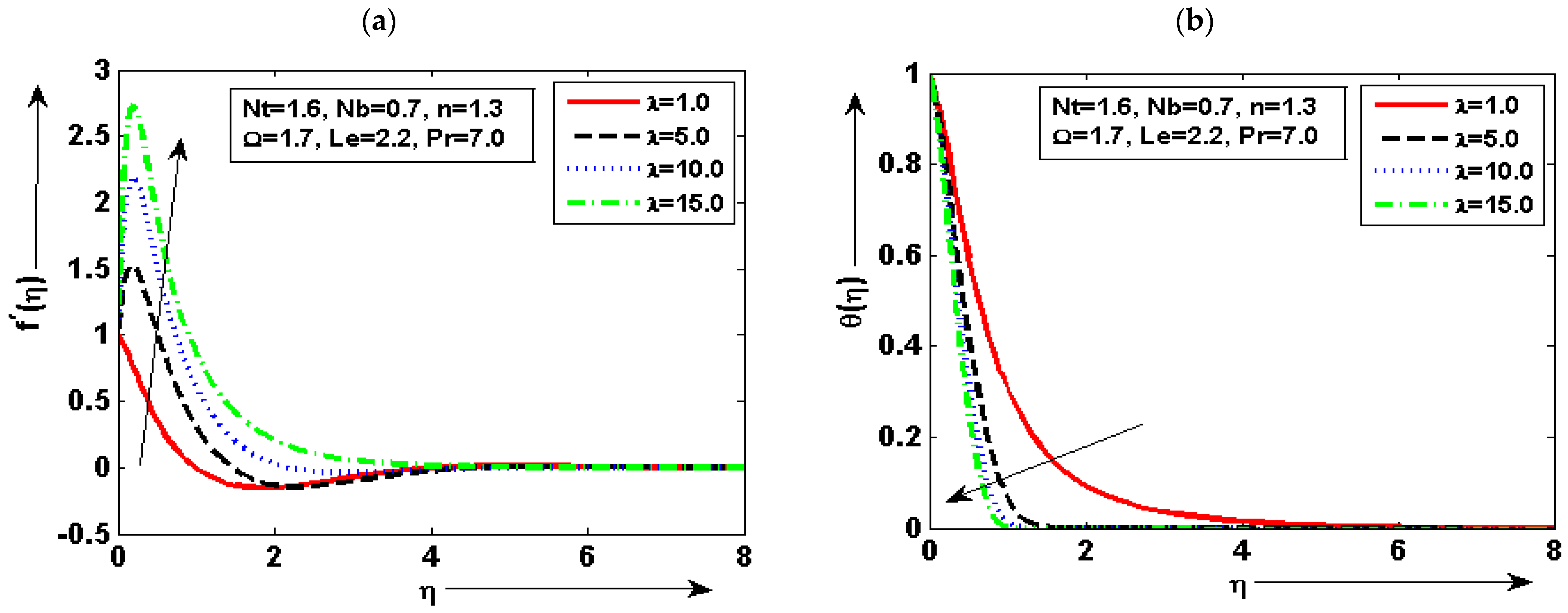
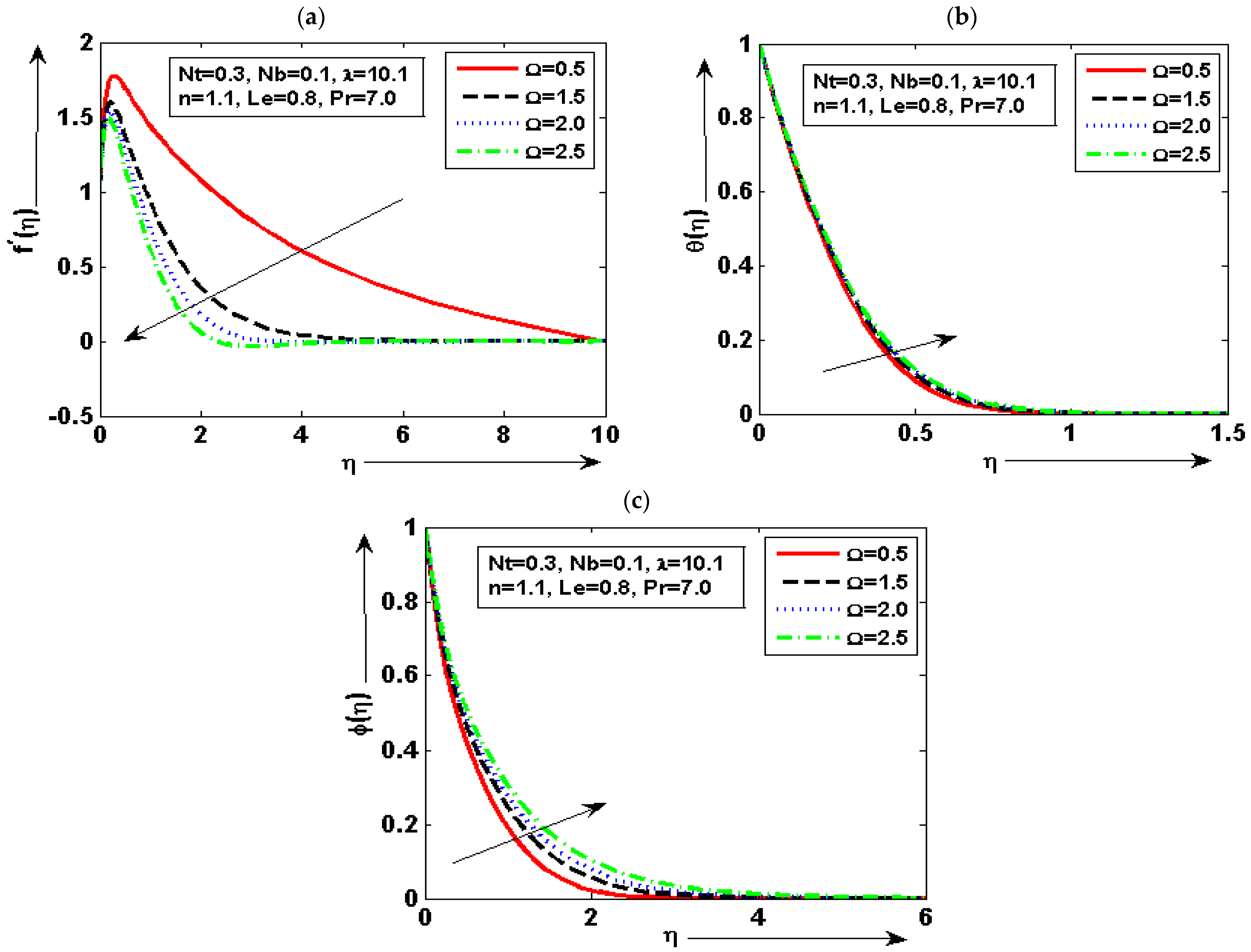
- It is noted that the velocity graph is maximum for the small quantity of and reduced for the larger by keeping the other parameters fixed. It can be seen that the temperature plot is enhanced for the maximum choice of and reduced for the minimum choice of ;
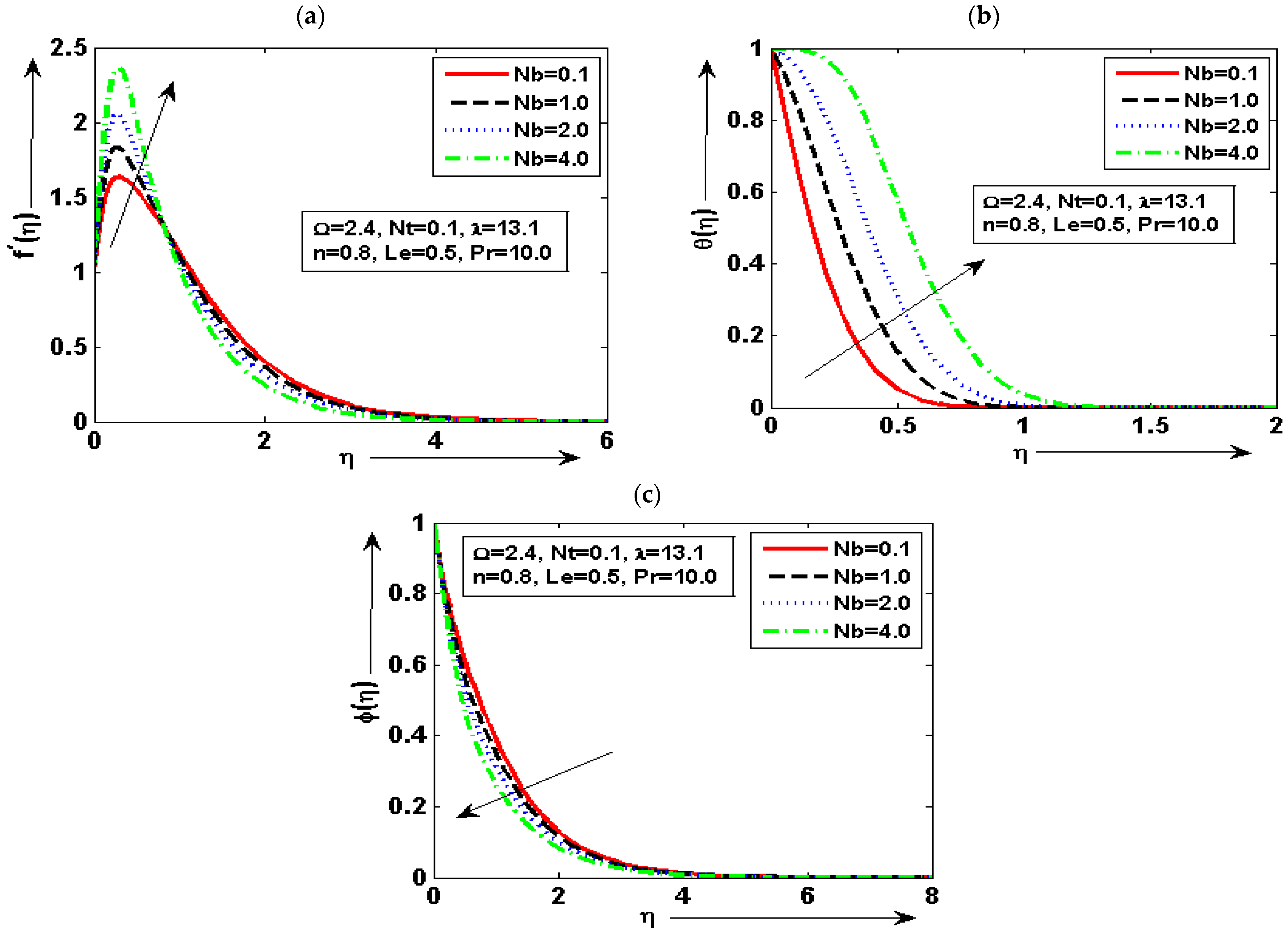
- The concentration graph is enhanced by decreasing but decreased by increasing . The skin friction is increased by increasing the value but decreased by decreasing the value of ;
- It is found that heat transfer is enhanced for the maximum choice of and the minimum choice at lower value of . It is also noted that mass transfer is enhanced due to increasing but reduced due to decreasing.
Author Contributions
Funding
Data Availability Statement
Conflicts of Interest
References
- Pourrajab, R.; Noghrehabadi, A. Bioconvection of nanofluid past stretching sheet in a porous medium in presence of gyrotactic microorganisms with newtonian heating. In MATEC Web of Conferences; EDP Sciences: Les Ulis, France, 2018; Volume 220, p. 01004. [Google Scholar]
- Sarkar, S.; Endalew, M.F. Effects of melting process on the hydromagnetic wedge flow of a Casson nanofluid in a porous medium. Bound. Value Probl. 2019, 2019, 43. [Google Scholar] [CrossRef]
- Kalavathamma, B.; Lakshmi, C. Effect of variable properties on heat and mass transfer flow of nanofluid over a vertical cone saturated by porous medium under enhanced boundary conditions. Int. J. Appl. Eng. Res. 2018, 13, 15611–15621. [Google Scholar]
- Dero, S.; Shaikh, H.; Talpur, G.H.; Khan, I.; Alharbim, S.O.; Andualem, M. Influence of a Darcy-Forchheimer porous medium on the flow of a radiative magnetized rotating hybrid nanofluid over a shrinking surface. Sci. Rep. 2021, 11, 24257. [Google Scholar] [CrossRef]
- Srinivasacharya, D.; Surender, O. Effect of double stratification on mixed convection boundary layer flow of a nanofluid past a vertical plate in a porous medium. Appl. Nanosci. 2015, 5, 29–38. [Google Scholar] [CrossRef]
- Ayodeji, F.; Abubakar, A.A.; Joy-Felicia, O.O. Effect of Mass and Partial Slip on Boundary Layer Flow of a Nanofluid over a Porous Plate Embedded In a Porous Medium. IOSR J. Mech. Civ. Eng. 2016, 13, 42–49. [Google Scholar] [CrossRef]
- Khan, W.A.; Pop, I. Boundary-layer flow of a nanofluid past a stretching sheet. Int. J. Heat Mass Transf. 2010, 53, 2477–2483. [Google Scholar] [CrossRef]
- Ghalambaz, M.; Noghrehabadi, A.; Ghanbarzadeh, A. Natural convection of nanofluids over a convectively heated vertical plate embedded in a porous medium. Braz. J. Chem. Eng. 2014, 31, 413–427. [Google Scholar] [CrossRef]
- James, M.; Mureithi, E.W.; Kuznetsov, D. Effects of variable viscosity of nanofluid flow over a permeable wedge embedded in saturated porous medium with chemical reaction and thermal radiation. Int. J. Adv. Appl. Math. Mech. 2015, 2, 101–118. [Google Scholar]
- Al-Farhany, K.; Al-Muhja, B.; Loganathan, K.; Periyasamy, U.; Ali, F.; Sarris, I.E. Analysis of Convection Phenomenon in Enclosure Utilizing Nanofluids with Baffle Effects. Energies 2022, 15, 6615. [Google Scholar] [CrossRef]
- Al-Mdallal, Q.; Prasad, V.R.; Basha, H.T.; Sarris, I.; Akkurt, N. Keller box simulation of magnetic pseudoplastic nano-polymer coating flow over a circular cylinder with entropy optimisation. Comput. Math. Appl. 2022, 118, 132–158. [Google Scholar] [CrossRef]
- Sofiadis, G.; Sarris, I. Reynolds number effect of the turbulent micropolar channel flow. Phys. Fluids 2022, 34, 075126. [Google Scholar] [CrossRef]
- Rana, P.; Bhargava, R. Flow and heat transfer of a nanofluid over a nonlinearly stretching sheet: A numerical study. Commun. Nonlinear Sci. Numer. Simul. 2012, 17, 212–226. [Google Scholar] [CrossRef]
- Irfan, M.; Farooq, M.A.; Iqra, T. A new computational technique design for EMHD nanofluid flow over a variable thickness surface with variable liquid characteristics. Front. Phys. 2020, 8, 66. [Google Scholar] [CrossRef]
- Ferdows, M.; Khan, M.; Alam, M.; Sun, S. MHD mixed convective boundary layer flow of a nanofluid through a porous medium due to an exponentially stretching sheet. Math. Probl. Eng. 2012, 2012, 408528. [Google Scholar] [CrossRef]
- Reddy Gorla, R.S.; Sidawi, I. Free convection on a vertical stretching surface with suction and blowing. Appl. Sci. Res. 1994, 52, 247–257. [Google Scholar] [CrossRef]
- Wang, C.Y. Free convection on a vertical stretching surface. J. Appl. Math. Mech. 1989, 69, 418–420. [Google Scholar] [CrossRef]
- Sandeep, N.; Sulochana, C.; Raju, K.; Babu, M.J.; Sugunamma, V. Unsteady boundary layer flow of thermophoretic MHD nanofluid past a stretching sheet with space and time dependent internal heat source/sink. Appl. Appl. Math. 2015, 10, 20. [Google Scholar]
- Khan, W.A.; Pop, I.M. Boundary layer flow past a stretching surface in a porous medium saturated by a nanofluid: Brinkman-Forchheimer model. PLoS ONE 2012, 7, e47031. [Google Scholar] [CrossRef]
- Alam, A.; Marwat, D.N.K.; Ali, A. Flow of nano-fluid over a sheet of variable thickness with non-uniform stretching (shrinking) and porous velocities. Adv. Mech. Eng. 2021, 13, 1–16. [Google Scholar] [CrossRef]
- Uddin, M.J.; Khan, W.A.; Amin, N.S. g-Jitter mixed convective slip flow of nanofluid past a permeable stretching sheet embedded in a Darcian porous media with variable viscosity. PLoS ONE 2014, 9, e99384. [Google Scholar] [CrossRef]
- Jafar, A.B.; Shafie, S.; Ullah, I. MHD radiative nanofluid flow induced by a nonlinear stretching sheet in a porous medium. Heliyon 2020, 6, e04201. [Google Scholar] [CrossRef]
- Prasannakumara, B.C.; Shashikumar, N.S.; Venkatesh, P. Boundary layer flow and heat transfer of fluid particle suspension with nanoparticles over a nonlinear stretching sheet embedded in a porous medium. Nonlinear Eng. 2017, 6, 179–190. [Google Scholar] [CrossRef]
- Narender, G.; Misra, S.; Govardhan, K. Numerical Solution of MHD Nanofluid over a Stretching Surface with Chemical Reaction and Viscous Dissipation. Chem. Eng. Res. Bull. 2019, 21, 36–45. [Google Scholar] [CrossRef]
- Dessie, H.; Fissha, D. MHD Mixed Convective Flow of Maxwell Nanofluid Past a Porous Vertical Stretching Sheet in Presence of Chemical Reaction. Appl. Appl. Math. 2020, 15, 31. [Google Scholar]
- Gireesha, B.J.; Mahanthesh, B.; Manjunatha, P.T.; Gorla, R.S.R. Numerical solution for hydromagnetic boundary layer flow and heat transfer past a stretching surface embedded in non-Darcy porous medium with fluid-particle suspension. J. Niger. Math. Soc. 2015, 34, 267–285. [Google Scholar] [CrossRef]
- Lakshmi, K.K.; Gireesha, B.J.; Gorla, R.S.; Mahanthesh, B. Effects of diffusion-thermo and thermo-diffusion on two-phase boundary layer flow past a stretching sheet with fluid-particle suspension and chemical reaction: A numerical study. J. Niger. Math. Soc. 2016, 35, 66–81. [Google Scholar] [CrossRef]
- Krishna, M.V.; Chamkha, A.J. Hall and ion slip effects on MHD rotating boundary layer flow of nanofluid past an infinite vertical plate embedded in a porous medium. Results Phys. 2019, 15, 102652. [Google Scholar] [CrossRef]
- Gireesha, B.J.; Mahanthesh, B.; Gorla, R.S.R. Suspended particle effect on nanofluid boundary layer flow past a stretching surface. J. Nanofluids 2014, 3, 267–277. [Google Scholar] [CrossRef]
- Maranna, T.; Sneha, K.N.; Mahabaleshwar, U.S.; Sarris, I.E.; Karakasidis, T.E. An Effect of Radiation and MHD Newtonian Fluid over a Stretching/Shrinking Sheet with CNTs and Mass Transpiration. Appl. Sci. 2022, 12, 5466. [Google Scholar] [CrossRef]
- Mabood, F.; Fatunmbi, E.O.; Benos, L.; Sarris, I.E. Entropy Generation in the Magnetohydrodynamic Jeffrey Nanofluid Flow Over a Stretching Sheet with Wide Range of Engineering Application Parameters. Int. J. Appl. Comput. Math. 2022, 8, 98. [Google Scholar] [CrossRef]
- Baranovskii, E.S. Flows of a polymer fluid in domain with impermeable boundaries. Comput. Math. Math. Phys. 2014, 54, 1589–1596. [Google Scholar] [CrossRef]
- Kakac, S.; Yener, Y. Convective Heat Transfer; CRC Press: Boca Raton, FL, USA, 1995; pp. 312–314, 399. [Google Scholar]


Disclaimer/Publisher’s Note: The statements, opinions and data contained in all publications are solely those of the individual author(s) and contributor(s) and not of MDPI and/or the editor(s). MDPI and/or the editor(s) disclaim responsibility for any injury to people or property resulting from any ideas, methods, instructions or products referred to in the content. |
© 2023 by the authors. Licensee MDPI, Basel, Switzerland. This article is an open access article distributed under the terms and conditions of the Creative Commons Attribution (CC BY) license (https://creativecommons.org/licenses/by/4.0/).
Share and Cite
Ullah, Z.; Aldhabani, M.S. Physical Analysis of Thermophoresis and Variable Density Effects on Heat Transfer Assessment along a Porous Stretching Sheet and Their Applications in Nanofluid Lubrication. Lubricants 2023, 11, 172. https://doi.org/10.3390/lubricants11040172
Ullah Z, Aldhabani MS. Physical Analysis of Thermophoresis and Variable Density Effects on Heat Transfer Assessment along a Porous Stretching Sheet and Their Applications in Nanofluid Lubrication. Lubricants. 2023; 11(4):172. https://doi.org/10.3390/lubricants11040172
Chicago/Turabian StyleUllah, Zia, and Musaad S. Aldhabani. 2023. "Physical Analysis of Thermophoresis and Variable Density Effects on Heat Transfer Assessment along a Porous Stretching Sheet and Their Applications in Nanofluid Lubrication" Lubricants 11, no. 4: 172. https://doi.org/10.3390/lubricants11040172
APA StyleUllah, Z., & Aldhabani, M. S. (2023). Physical Analysis of Thermophoresis and Variable Density Effects on Heat Transfer Assessment along a Porous Stretching Sheet and Their Applications in Nanofluid Lubrication. Lubricants, 11(4), 172. https://doi.org/10.3390/lubricants11040172