Research on Simulation Method for Wear for Dynamic Seal in Axial Flux Hub Motor

Abstract

A simulation method for the wear of a dynamic seal in an axial flux hub motor is proposed in this work. A quasi-3D magnetic model without deflection between the axes of a stator and a rotor is built. An analytical model for unbalanced magnetic force considering the cogging effect and axial deflection is presented based on the quasi-3D magnetic model. Boundary conditions of the dynamic seal are obtained through solving the FE model of a hub motor. Both the structural and thermal FE model of a dynamic seal are built and the thermal–structural coupling method is given. A dynamic wear simulation method is displayed based on the mesh reconstruction method proposed previously. It is proved through the contrast with the experimental results that the presented method is feasible.

1. Introduction

As new energy vehicles develop, the driving technology of the hub motor is widely applied. Since they own a high magnetic flux density and large output torque, axial flux hub motors (AFHMs) have been paid more attention in the new energy vehicle field [1,2]. Dynamic seals are one of the most important components in AFHMs. Clearance between the stator and rotor is filled by them. As installed in wheels that are close to the ground, AFHMs face a variety of complicated environments (such as ice, stones, etc.). Once dynamic seals no longer work, AFHMs do not rotate normally and the security of the whole car is seriously threatened.

As is known, errors cannot be avoided in the manufacturing and assembling of AFHMs. Thus, distribution of the magnetic field in the clearance of an AFHM will not be even. According to the Maxwell stress tensor, the unbalanced magnetic force (UMF) will emerge in the AFHM and lead to an installation error of the dynamic seal. The dynamic seal contacts with the opposite surfaces unevenly and uneven wear may come out. An finite element (FE) model of AFHM was built by Marignetti [3] and distribution of the magnetic field with axes deflection of the AFHM was simulated. Although the FE method was convenient for modelling distribution of the magnetic field, a high computer resource was occupied and the efficiency was low. An analytical model of a magnetic field was presented by Bellini [4]. This model was well accepted by electric motor designers. However, much time was still needed to solve the model [5]. A field reconstruction method was proposed by other researchers [6,7]. This was a method that solved the analytical model and three dimensional FE model together. It was more efficient than modelling merely through the FE method. However, much time was still required. An analytical model of the distribution of a magnetic field for an AFHM was built by Huang [8]. The cogging effect was taken into consideration and the axes error was chosen as the input parameter. An uneven distribution of the magnetic field in clearance was solved quickly. However, the influence of an uneven magnetic field on the wear of the dynamic seal was not paid attention to.

Studies on seal wear have been focused on by researchers [9,10,11]. The wear process of a dynamic seal, which moves reciprocally in hydraulic equipment, was simulated by Angerhausen [12]. The wear loss was calculated based on Archard’s model. The oil film effect was considered. The wear process of a dynamic seal was calculated iteratively based on Reynolds equation and Persson’s contacting theory. The multiscale simulation method was adopted to model the wear process of the lip seal under a mixed lubricated state by Liu [13]. The relationship between wear loss and the distribution of the abrasiveness in the radial and circumferential directions was obtained. The effect of the size and distribution of abrasive particles on the wear loss of the dynamic seal was studied through an experimental method by Shen [14]. The experimental method was also used by Guoqing [15] to study the wear characteristics of a finger seal in an aero motor under both high and low temperature environments. Leakage performance was studied as well. Although wear characteristics of a dynamic seal can be predicted precisely through the experimental method, it takes time to set up a test bed, which is sometimes infeasible. The simulation method can not only save on the time cost, but also obtain results that are difficult or impossible to measure under the experimental conditions through the coupling of multiple physical fields. The existing simulation methods often focus on the sealing system with a lubricant, while the normal working condition of the AFHM is the dry friction system without a lubricant. Therefore, the existing research results cannot be consistent with the working conditions of the AFHM.

As introduced above, a wear method of a dynamic seal in an AFHM will be proposed in this work. Firstly, a model of a UMF for an AFHM is built considering both the cogging effect and axes deflection between a stator and rotor. The installation boundary of the dynamic seal is obtained by solving the FE model of the AFHM. The FE models of a dynamic seal in both the structural field and thermal field are established. The dynamic wear simulation method of a dynamic seal is given by using the thermal–solid coupling solution method and mesh reconstruction technology. Finally, the feasibility of the proposed method is verified by experiments.

2. Model of UMF for AFHM

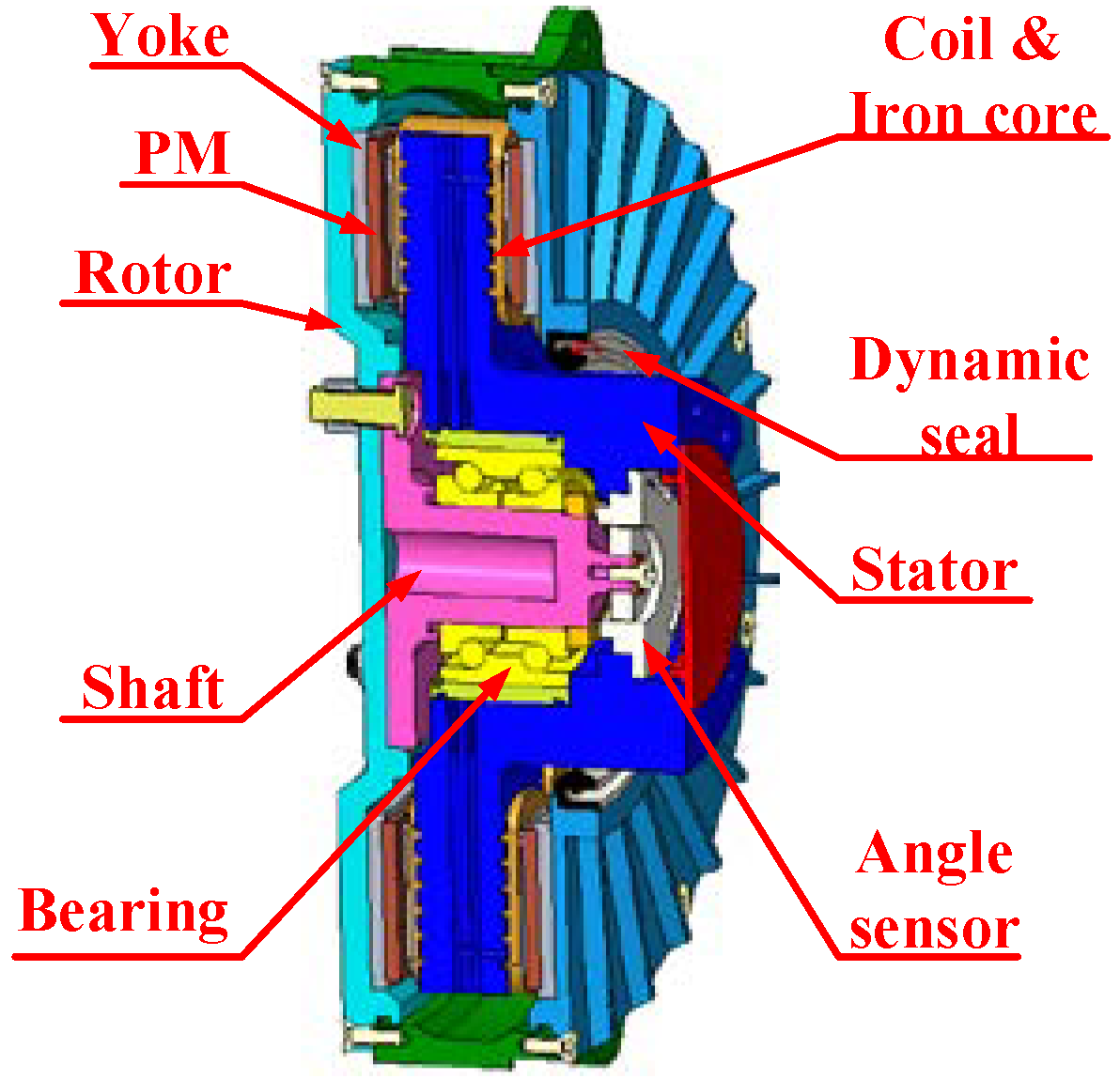
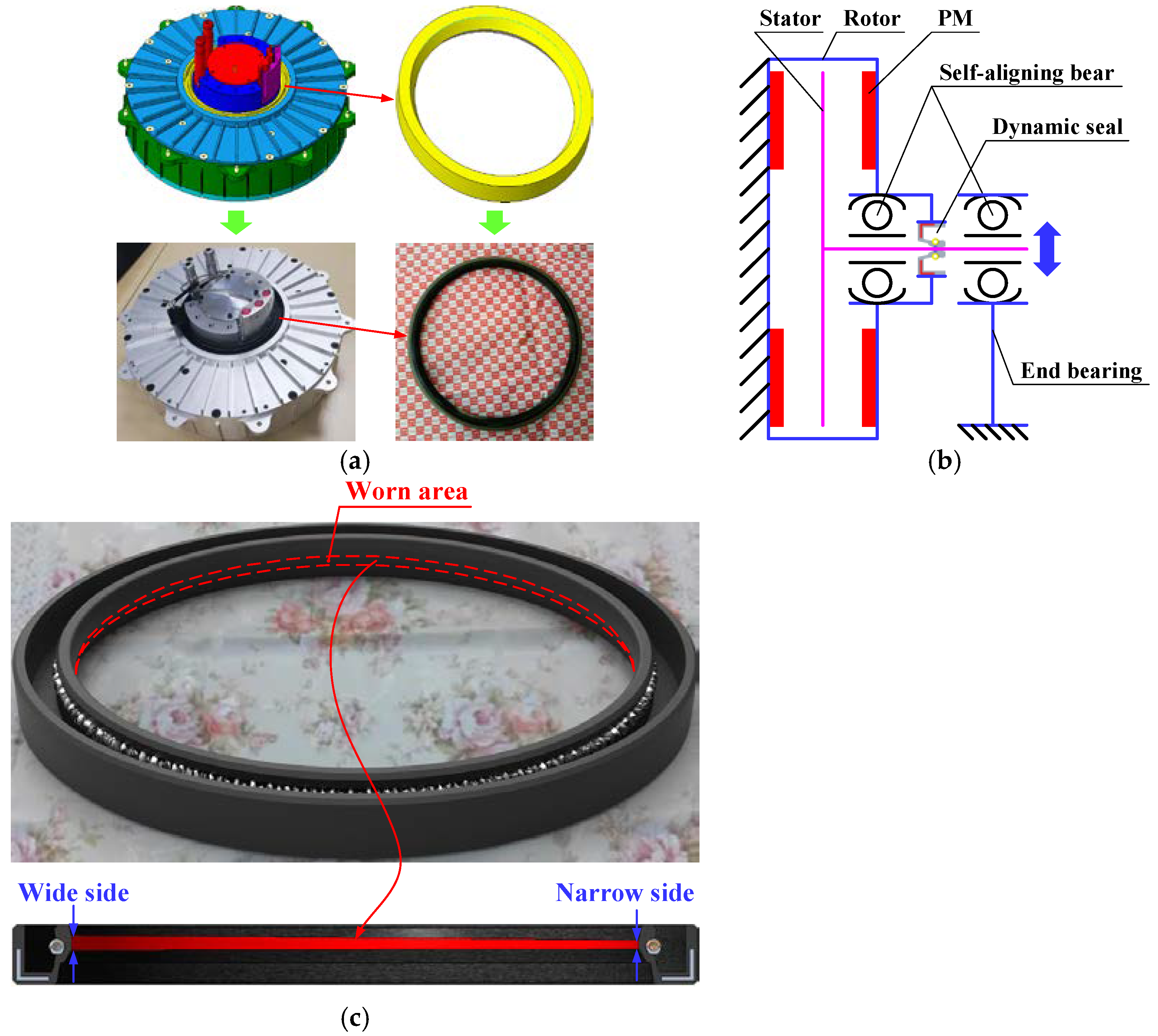
A hub motor is the core component of new energy vehicles. Nowadays, the common form of a hub motor in new energy vehicles is the AFHM. Due to its high power density and small axial size, it can be directly installed in the rim as a power output element. The typical structure of an AFHM is with an outer rotor and inner stator, as shown in Figure 1. The main magnetic field direction of the permanent magnets (PMs) is distributed along the axis. The stator is located inside, while the rotor is located outside. The dynamic seal is installed between the stator and the rotor.

According to the working conditions of a hub motor, a dynamic seal works in a dry friction state mostly. Since the hub motor rotates fast, the dynamic seal is easily worn. In fact, due to the influence of machining error, loading deformation and so on, a deflection error will emerge between the stator and the rotor. Distribution of the magnetic field will not be even any more. As the electrifying windings move in the magnetic field, the wave caused by Ampere’s force will affect the wear performance of the seal. Thus, the deflection error between the stator and rotor needs to be considered during an analysis of the wear process of a dynamic seal.

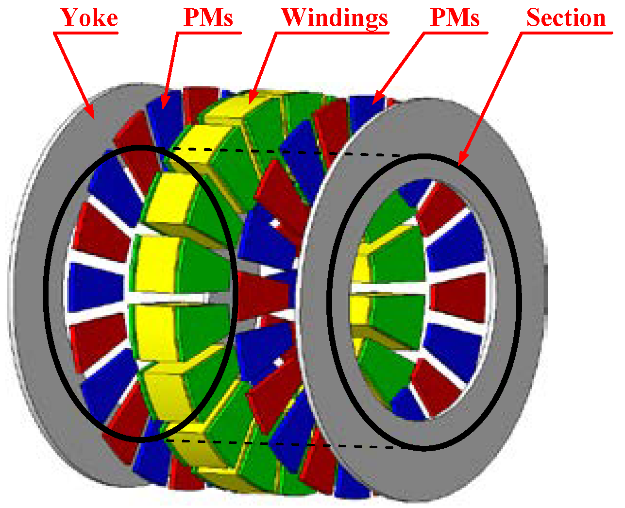
To find out how the deflection error affects the wave of Ampere’s force, a quasi-3D magnetic model of an AFHM was built first. Based on the thought of dimension reduction, the magnetic field of the AFHM was divided into some cylindrical surfaces, as shown in Figure 2, and every cylindrical surface flattened. Then, the magnetic field of AFHM was taken as a combination of linear PM motors without an edge effect.

The average radius of each cylindrical surface is

$$R_{av}=R_i+\frac{R_o-R_i}{n_s}\left(i-\frac{1}{2}\right),i=1,2,\dots ,n_s$$

(1)

where n_s is the number of equivalent liner PM motors.

For convenience, the cogging effect is neglected and the following assumptions are made:

(1)

materials of PMs and iron core are isotropic and the PMs is magnetized uniformly;

(2)

demagnetization curve of PMs is linearly distributed;

(3)

the relative permeability of ferromagnetic materials is infinite;

(4)

both current and end effect are ignored.

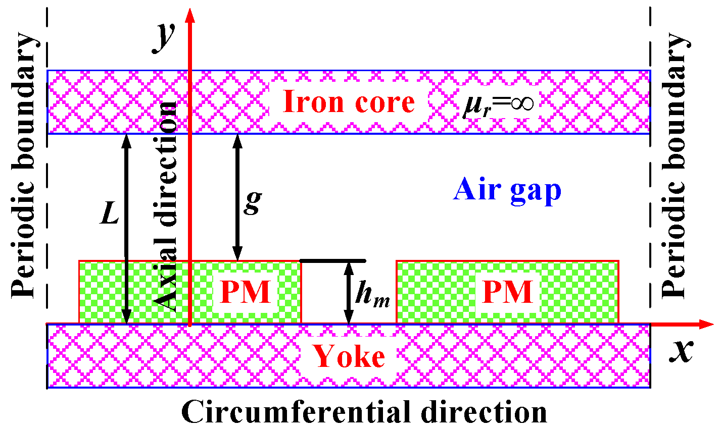
Based on the above assumptions, the multi-section method is used to establish the magnetic field domain analytical model, as shown in Figure 3. The Ampere’s force acts on the iron core and its coils through the magnetic field in the air gap. Therefore, the magnetic field distribution in the air gap is mainly concerned in the magnetic field domain analytical model. According to the Maxwell stress tensor method, the magnetic field distribution in the air gap is

$$\begin{array}{l}{B}_x={\displaystyle \sum _{n=1,3,5}^{\infty }{\mu }_0{M}_n\frac{\sin h\left(K_n{h}_m\right)}{\Delta }\sin h\left[K_n\left(L-y\right)\right]\sin \left(K_{n}x\right)}\\ B_y={\displaystyle \sum _{n=1,3,5}^{\infty }{\mu }_0{M}_n\frac{\sin h\left(K_n{h}_m\right)}{\Delta }\cos h\left[K_n\left(L-y\right)\right]\cos \left(K_{n}x\right)}\end{array}$$

(2)

where

$$\Delta ={\mu }_r\cos h\left(K_n{h}_m\right)\sin h\left(K_{n}g\right)+\sin h\left(K_n{h}_m\right)\cos h\left(K_{n}g\right)$$

(3)

$$M_n=\frac{4B_r}{n\pi {\mu }_0}\sin \left(\frac{n\pi {\alpha }_p}{2}\right)$$

(4)

where B_r is residual magnetic field strength of PMs, μ₀ is vacuum permeability, μ_r is reversion permeability, α_p is pole arc coefficient.

$$K_n=\frac{n\pi }{{\tau }_p}$$

(5)

$${\tau }_p=\frac{\pi R_{av}}{p}$$

(6)

where τ_p is polar distance and p is the number of pole pairs.

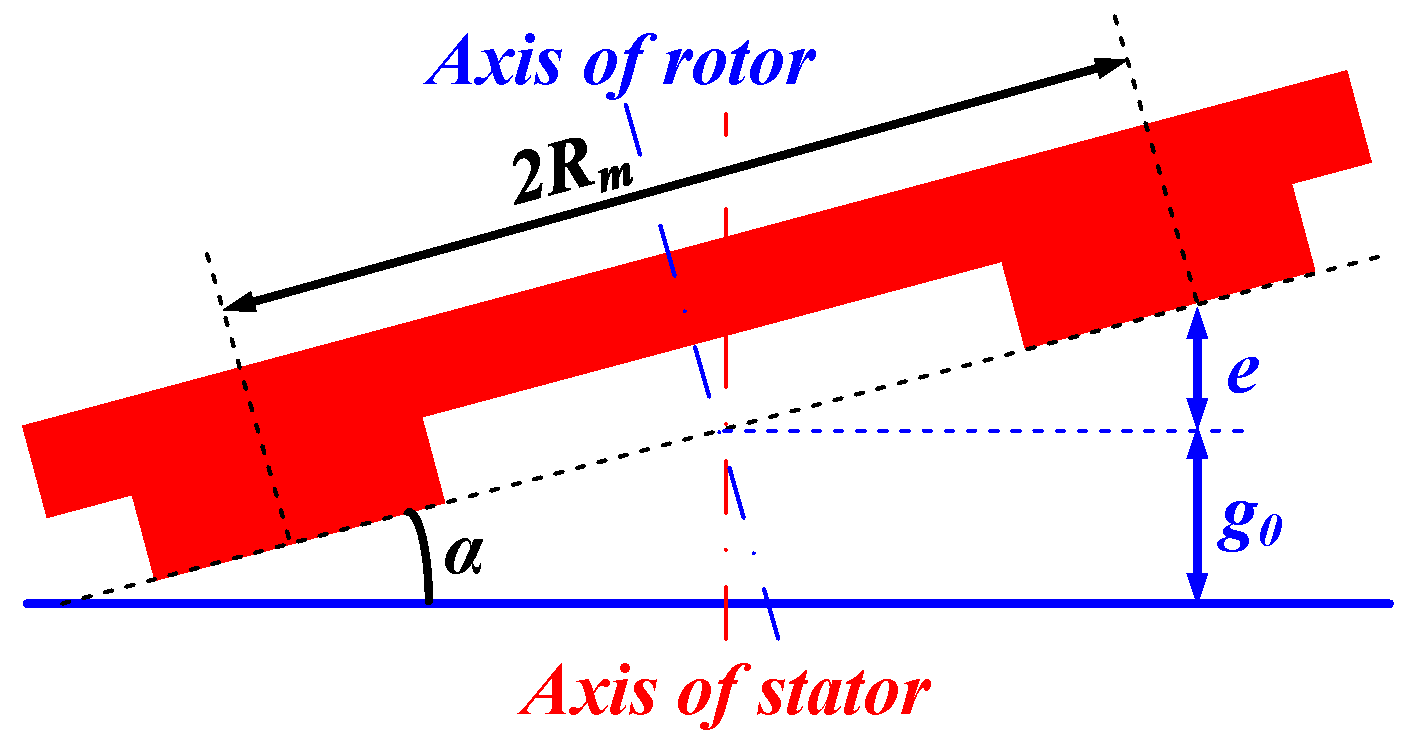
The cogging effect is not considered in the analytical model given above. According to [16], the cogging effect can be accurately reflected by complex conformal transformation. The air gap distribution will no longer be uniform once the axes of the stator and rotor are not coinciding, as shown in Figure 4. The static deflection coefficient is defined as

$$\mathrm{SEF}=\frac{e}{g_0}\times 100\%$$

(7)

where e is the maximum value of the air gap increment and g₀ is the thickness of the air gap without axis deflection.

When the axis of the axial flux motor deflects, the air gap thickness distribution at the average radius can be expressed as

$$g_m\left(\theta \right)=g_0-e\cos \left(\theta -{\gamma }_0\right)=g_0\left[1-\mathrm{SEF}\cos \left(\theta -{\theta }_0\right)\right]$$

(8)

where θ₀ represents the location where the minimum thickness of the air gap emerges.

Due to the axis deflection, the air gap thickness at different radii is also different. According to Equation (8) and Figure 4, the air gap thickness at different radii is

$$g\left(R,\theta \right)=g_m\left(\theta \right)-\left(R-R_m\right)\sin \alpha \cos \left(\theta -{\theta }_0\right)=g_0\left[1-\frac{R}{R_m}\mathrm{SEF}\cos \left(\theta -{\theta }_0\right)\right]$$

(9)

where R_m is the average radius of PMs.

Through Equations (2)–(6) and (9) and complex conformal transformation, the air gap magnetic field distribution can be obtained. According to the Maxwell stress tensor method, the axial force wave is

$$P_y\left(R,\theta \right)=\frac{B_y^2\left(R,\theta \right)-B_x^2\left(R,\theta \right)}{2{\mu }_0}$$

(10)

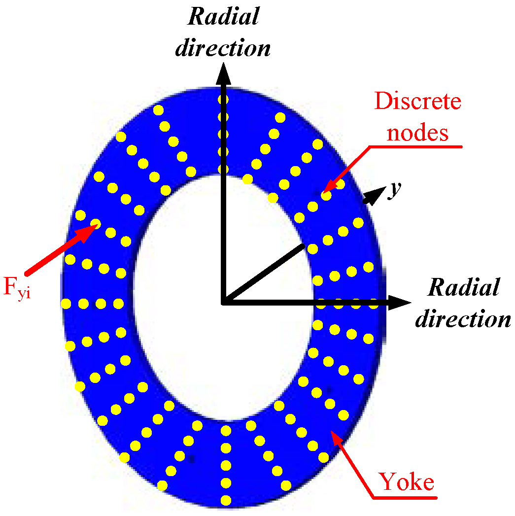
The UMF acting on the rotor is the product of the axial force wave and area, as shown in Figure 5. Considering the cogging effect, the electromagnetic field does not change continuously in space. Thus, the UMF is expressed in discrete form as

$$F_y\left(R,\theta \right)=P_y\left(R,\theta \right)\Delta S=P_y\left(R,\theta \right)r\Delta \theta \Delta r$$

(11)

where r is the distance from the discrete node to the center of the motor. Δr and Δθ are the increment of the distance and angle, respectively.

Then, discrete points on the rotor plane are selected as the action points of UMF. The deformation of the rotor under UMF can be simulated, as shown in Figure 6.

3. Dynamic Wear Simulation Method of Dynamic Seal

The dynamic seal will make contact with the mating surface in a dry friction state when the stator and rotor move relative to one another. The wear process of the dynamic seal will be heavily impacted by friction heat due to the high relative speed. In order to consider the influence of friction heat, the FE method is used to carry on the thermal–solid coupling simulation.

The dynamic seal is made of rubber. To consider the hyperelasticity of rubber, the Mooney–Rivlin model is adopted. The mating surfaces are made of metal. Since their hardness and elastic modulus are much greater than those of rubber materials, the mounting groove of the dynamic seal is treated as a rigid boundary constraint in the FE model. The axis deflection between the stator and rotor also needs to be considered. The structural FE model of the dynamic seal is shown in Figure 7. In order to reduce the amount of calculation, only half of the FE model is established according to the symmetry. Possible contact surfaces between the stator and the dynamic seal are set as contact pairs firstly. The deflected stator is moved in the axial direction of the seal to model the installation of the dynamic seal. The contact pressure between the seal and the stator can be gradually solved.

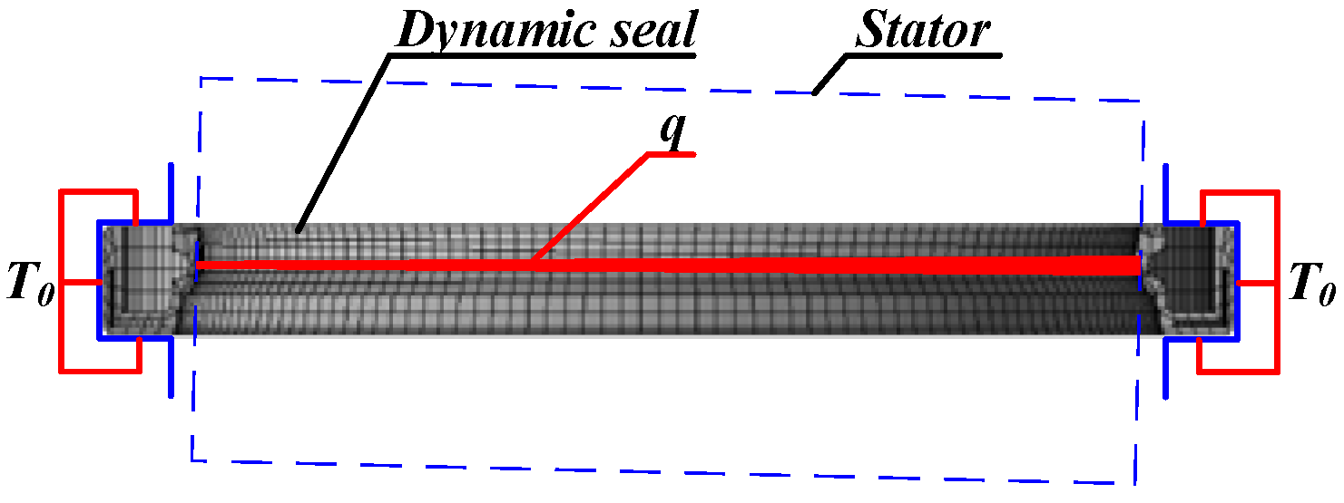
Then, the thermal field of the dynamic seal is analyzed. The thermal FE model of the dynamic seal is established based on the node coordinates on the outer profile after the contact deformation, as shown in Figure 8. The initial ambient temperature is set as T₀. To model the effect of friction heat, the heat flux is set on the contact surface. According to [17,18,19], the friction heat flux at each node can be expressed as

$$q_i=\psi f{p}_{i}u$$

(12)

where ψ represents the proportion of the mechanical work converted into friction heat. According to [20], the whole mechanical work can be taken as converted into friction heat, meaning ψ = 1.0. f is the coefficient of the dynamic friction between the dynamic seal and the stator. p_i is the normal pressure of the contact nodes. u is the relative speed.

The structural equations and thermal equations for the dynamic seal need to be solved coupled. The bond effect between the dynamic seal and the stator is ignored. The equilibrium equation in the structural field can be expressed as

$$KU=F$$

(13)

where U is the vector of displacement. K is the matrix of stiffness. F is the vector of load. F is composed of two parts: external load, F_a, and thermal load F_t. F_t is defined as

$$F_t=\phi T$$

(14)

where T is the vector of nodal temperature. φ is thermal strain and it is expressed as

$$\phi =\alpha \left(T-T_0\right)\left[111\right]$$

(15)

where α is the coefficient of thermal expansion and T₀ is the initial ambient temperature.

Nodal displacement can be written as following according to Equations (13) and (14)

$$U=K^{-1}\left(F_a+\phi T\right)$$

(16)

The equilibrium equation in i-th element is

$$K^i{U}^i=F^i$$

(17)

The displacement of element, Uⁱ, can be obtained with the three order matrix, $Z_T^i$, and the total displacement, U.

$$U^i=Z_T^{i}U$$

(18)

Similarly, the vector of load in element i can be given as

$$F^i=F_{ap}^i+{\phi }^i{T}^i$$

(19)

where Tⁱ = $Z_T^i$T and $F_{ap}^i$ = [Pⁱ $F_a^i$]’. Pⁱ is the pressure vector of the contact node, while $F_a^i$ is the component of the external load in the i-th element.

The pressure of the contact node in element i can be given according to Equations (16) and (19)

$$P^i=A^{i}T+B^i{F}_a$$

(20)

where

$$A^i=-{\phi }_1^i{Z}_T^i+\left[K_{11}^i{K}_{12}^i{K}_{13}^i\right]Z^i{K}^{-1}\phi$$

$$B^i=\left[K_{11}^i{K}_{12}^i{K}_{13}^i\right]Z^i{K}^{-1}$$

$K_{ij}^i$(i, j = 1,2,3) is the stiffness matrix of the dynamic seal field.

The thermal equilibrium equation in i-th element is

$$c^i{\rho }^i\frac{\partial T^i}{\partial t}-k^i{\nabla }^2{T}^i=0$$

(21)

where t is time, c is the specific heat of seal, ρ is density and k is thermal conductivity.

The initial ambient temperature, T₀, is set as the initial condition, while the heat flux, q, is chosen as the boundary condition.

$$-k^i\frac{\partial T^i}{\partial n}=q^i$$

(22)

In the FE model, the thermal equilibrium equation of the dynamic seal field is given as

$$C\dot{T}+L_{D}T+Q=0$$

(23)

where C is the matrix of specific heat, L_D is the matrix of heat conduction and Q is the vector of the thermal load

$$C={\displaystyle \int c^i{\rho }^{i}WNdV}$$

$$L_D={\displaystyle \int k^i\nabla W\nabla NdV}$$

$$Q={\displaystyle \int W{k}^i\frac{\partial T^i}{\partial n}ds}$$

Since the temperature gradient between the adjacent elements, i and j, is continuous, it can be seen according to energy conservation law that

$${k^i\frac{\partial T^i}{\partial n}|}_{{\Omega }^i}-{k^j\frac{\partial T^j}{\partial n}|}_{{\Omega }^j}=q^{ij}$$

(24)

q^ij is the difference in heat flux.

The structural–thermal coupled method can be obtained through Equations (12), (20) and (23)

$$C\dot{T}+\left(L_D+fuA\right)T=-fuB{F}_a$$

(25)

The above equation can be transformed into

$$\dot{T}-GT=S{F}_a\left(t\right)$$

(26)

where

$$G=-C^{-1}\left(L_D+fuA\right)$$

(27)

The nodal temperature in the dynamic seal field can be solved through Equation (26), and then the contact pressure is obtained through Equation (20).

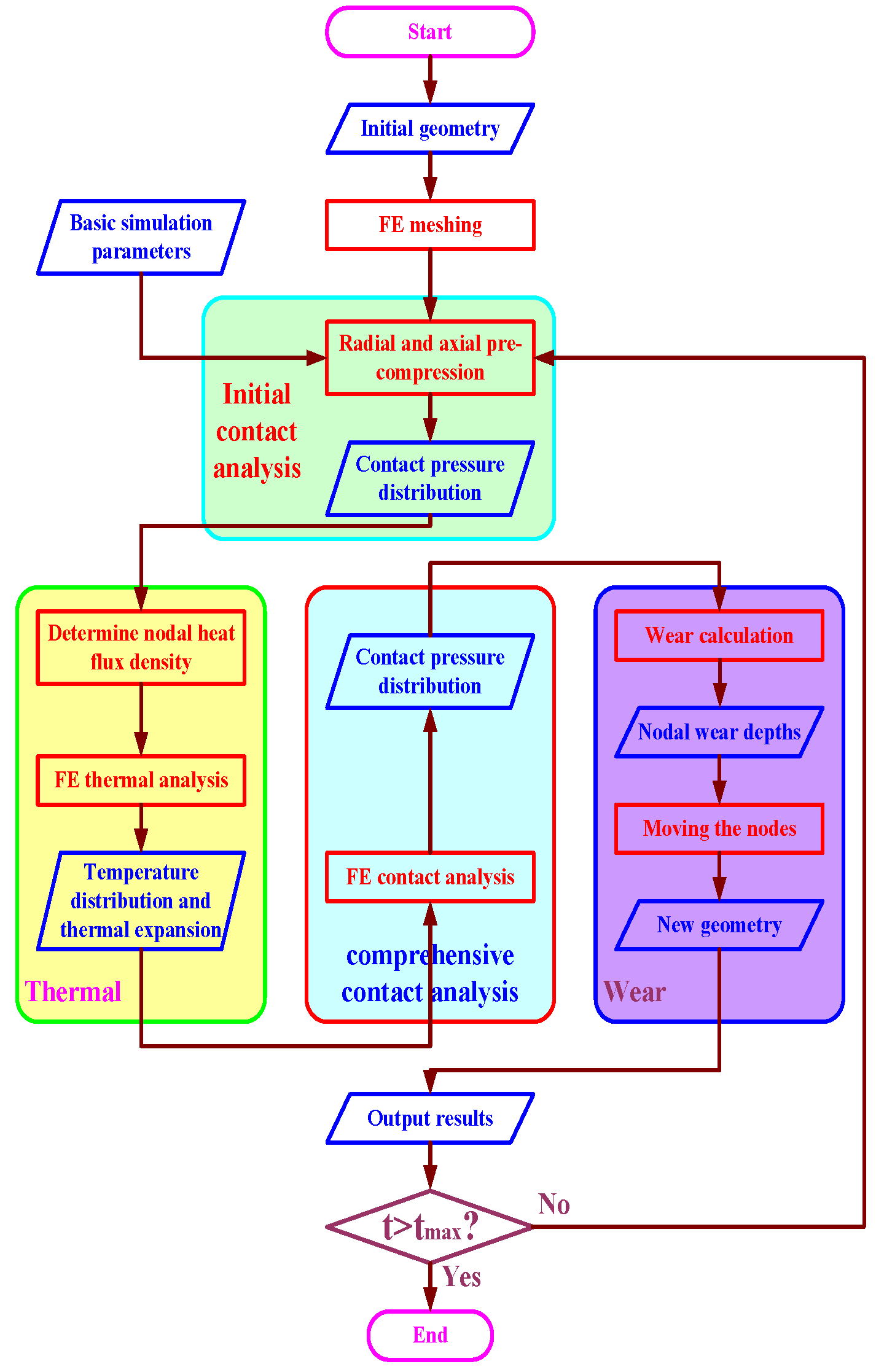
The wear depth of the seal is calculated based on Archard’s model. A previous achievement, the technology of mesh reconstruction, presented in [21] by the author, is adopted. Combining with the structural–thermal coupled calculation in the dynamic seal field, the method of dynamic wear simulation for the dynamic seal is displayed in Figure 9. Four modules are included: initial contact analysis, thermal analysis, comprehensive contact analysis and wear simulation. According to the predefined period, the wear amount of the dynamic seal can be modeled during this period.

4. Experiment for Wear of Dynamic Seal in AFHM

An experiment on the wear of a dynamic seal in an AFHM is carried out in this work. The purpose of the experiment is to validate whether the method presented above is feasible. The AFHM and dynamic seal in it are shown in Figure 10a. The outer diameter of rotor is 350 mm. The thickness of rotor is 80 mm. The weight of AFHM is less than 33 kg. The outer diameter of dynamic seal is 170 mm and its thickness is 15 mm. The no-load speed of motor is 2850 rpm. The process of experiment is accomplished on a specific test rig designed for AFHM. Its sketch map is shown in Figure 10b. The rotor of AFHM is fixed, while the stator is installed in end bearing through a self-aligning bear. The rolling bear in AFHM between stator and rotor is replaced by a self-aligning bear with the same size as the origin rolling bear. The value of SEF can be changed via modifying the height of end bearing according to the size of AFHM. The motor rotates under no-load speed for specific periods. Then disassemble the dynamic seal out of AFHM. Record the profile of the worn dynamic seal. Reinstall a new dynamic seal and reassign the rotating period. Once time is reached, disassemble the seal and record its worn profile. Repeat this process and the worn profile of dynamic seal at different time will be obtained. The worn area of dynamic seal is displayed in Figure 10c.

5. Results and Discussion

Results and discussions are provided in this section. Parameters used in the simulation are listed in

Table 1. Parameters used in the simulation.

Parameters	Value
Residual magnetic field strength of PMs Br (T)	1.23
Outer diameter of PMs Ro (mm)	150
Inner diameter of PMs Ri (mm)	93
Vacuum permeability μ0 (H/m)	4π × 10−7
Reversion permeability μr	1.05
Pole arc coefficient αp	0.83
Number of pole pairs p	20
Ideal axial distance between yoke and iron core L (mm)	6.2
Thickness of PMs hm (mm)	5.0
Elastic modulus of dynamic seal E (MPa)	7.84
Poisson’s ratio of dynamic seal υ	0.49
C01 in Mooney–Rivlin model (MPa)	72.33
C10 in Mooney–Rivlin model (MPa)	289.33
Density of dynamic seal ρ (103 kg/m3)	1.4
Thermal conductivity of dynamic seal k (W/m °C)	0.16
Specific heat of dynamic seal c (J/kg °C)	1700
Thermal expansion coefficient of dynamic seal α (°C−1)	6.9 × 10−4
Elastic modulus of stator and rotor (GPa)	72
Poisson’s ratio of stator and rotor	0.33
Ambient temperature T0 (°C)	25
Coefficient of dynamic friction f	0.3
Wear coefficient of seal (mm3/Nm)	7.2 × 10−6

.

The distribution of the magnetic field under an ideal state in the air gap along the axial direction and circumferential direction of the AFHM is displayed in Figure 11. The strength of the magnetic field at different heights of the air gap is shown. The cogging effect affects the strength of the axial magnetic field. It can be seen from Figure 11b that the strength of the circumferential magnetic field is larger near the surface of PMs, while being smaller close to the surface of the iron core.

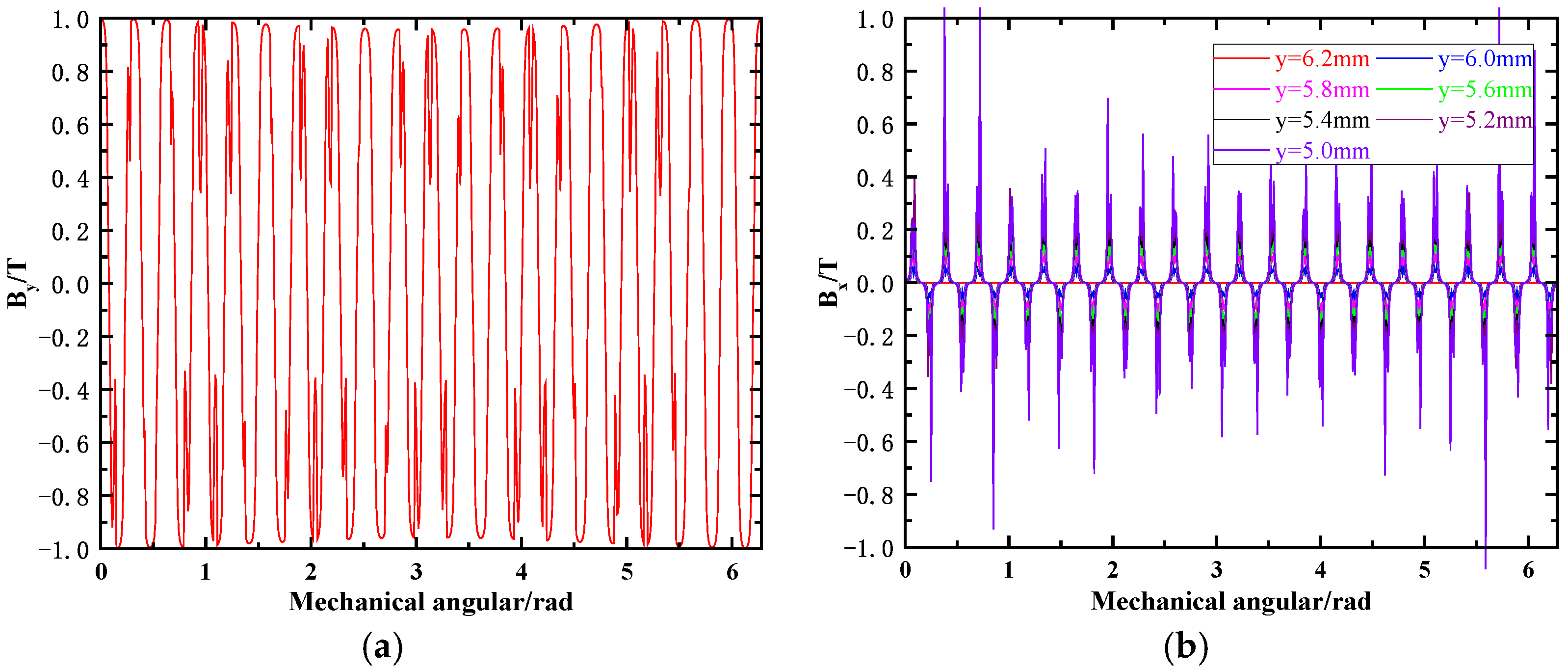
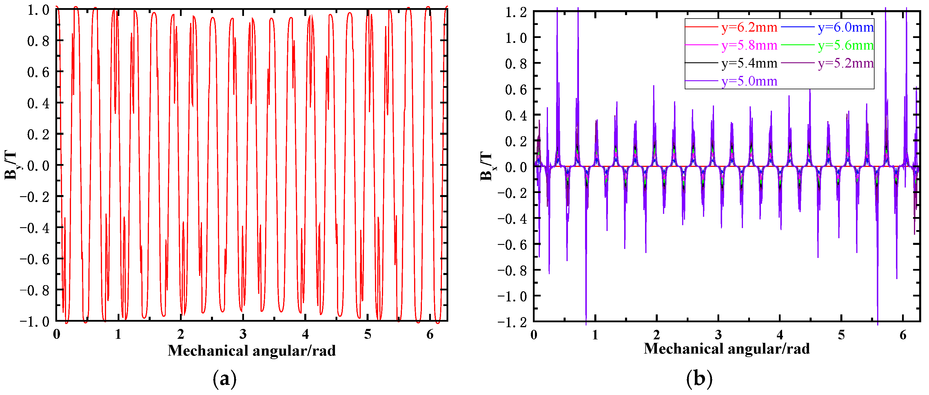
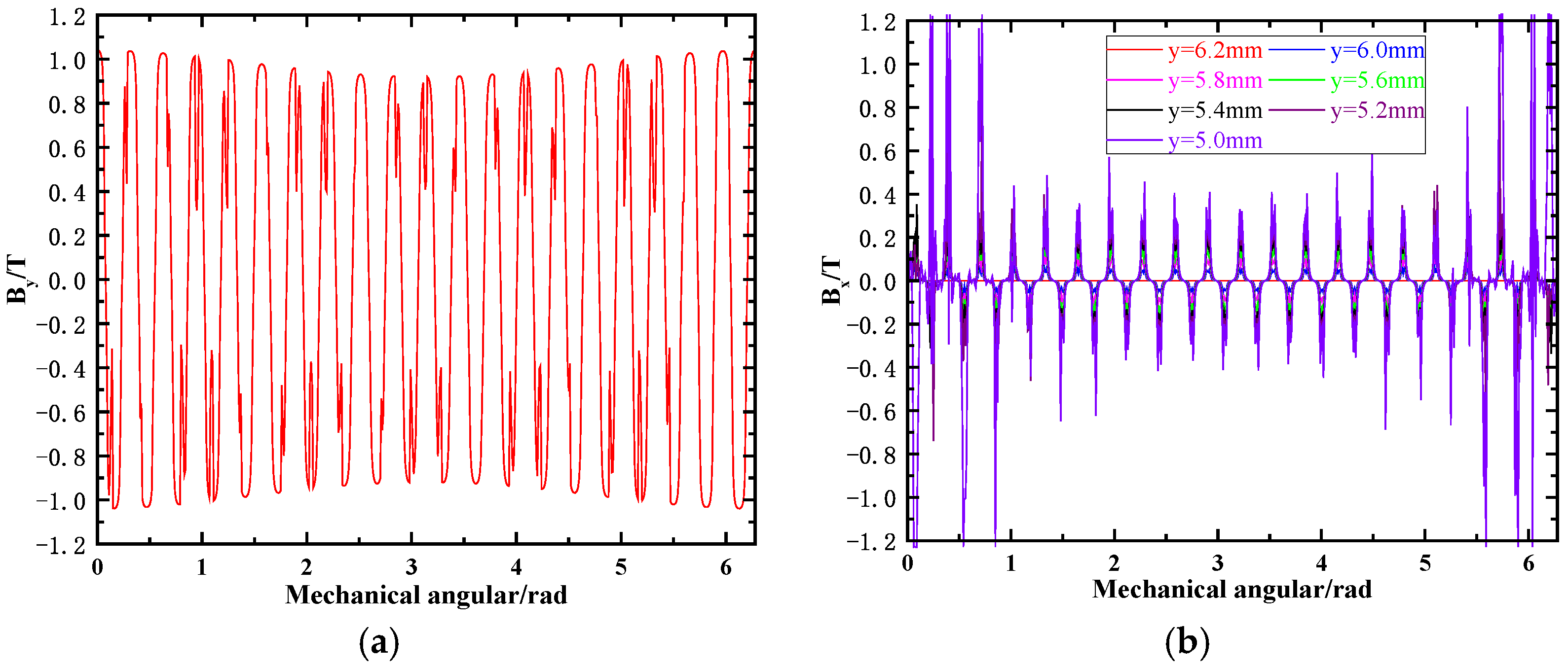
Distribution of both THE axial magnetic field and circumferential magnetic field with axes deflection is plotted in Figure 12, Figure 13 and Figure 14. While designing and assembling the AFHM, the static deflection coefficient can be controlled below 25% through selecting proper process parameters. Therefore, 8.33%, 16.67% and 25% are set as the input parameters of SEF. The mechanical angle where the thickness of the air gap is at its minimum is assumed as θ₀ = 0°. We can find from different results that the distribution of the axial magnetic field waves increases obviously as SEF is increased. When SEF reaches 25%, the maximum strength of the magnetic field at different mechanical angles already shows fairly obvious waviness. The strength of the magnetic field is larger as the thickness of the air gap becomes smaller. A similar tendency also happens to the circumferential magnetic field distribution. The maximum strength of the magnetic field emerges at which the minimum air gap stays.

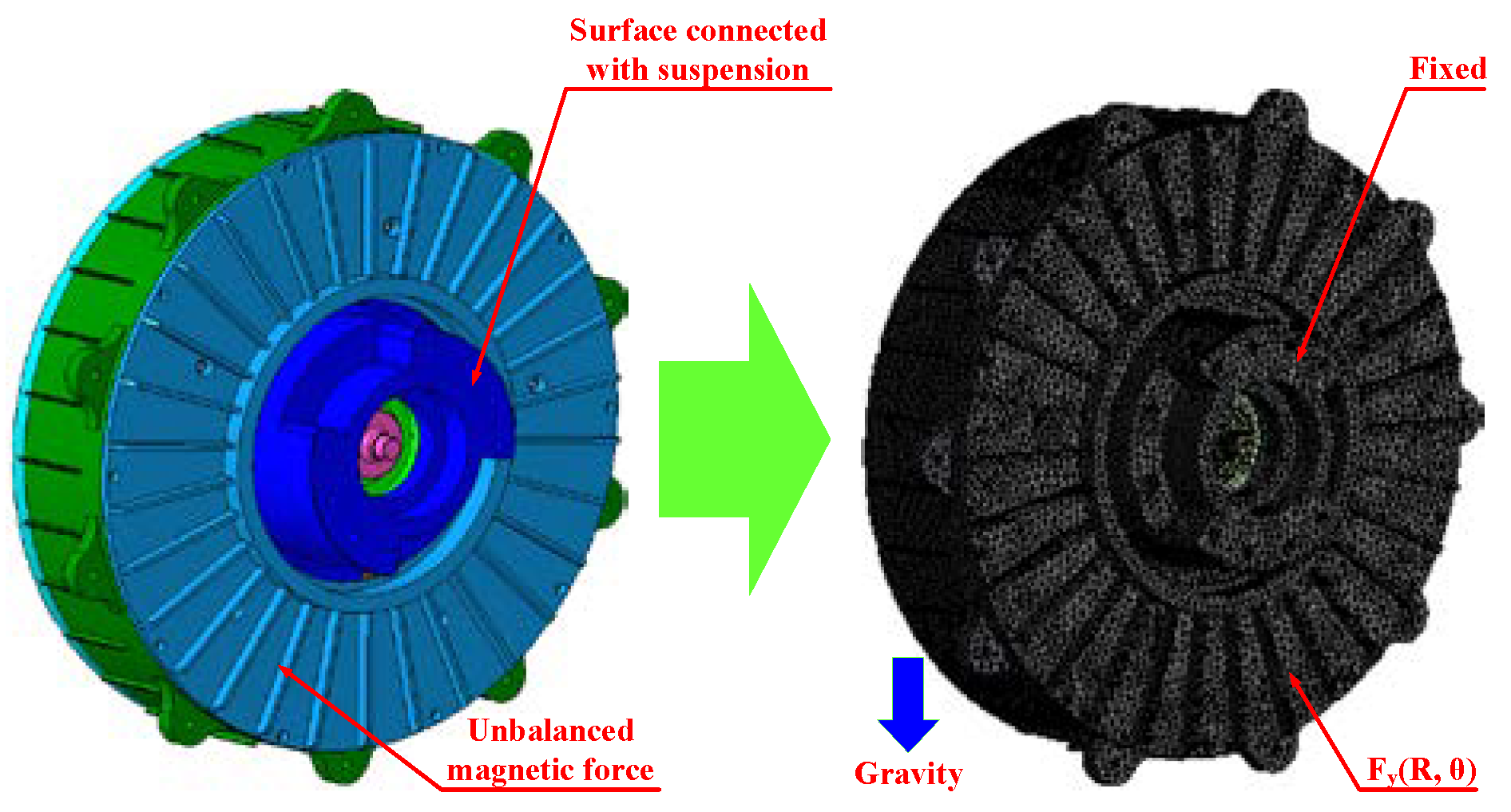
The FE model of the AFHM is built according to the no-load working conditions as shown in Figure 15. Since the end face of the stator is fixed with the suspension in a real car, the fixed constraint boundary condition is set on the end face of the stator. UMF is set on the surface of the yoke according to Equation (11). To take gravity into consideration, gravitational acceleration along the vertical direction is set as the initial condition.

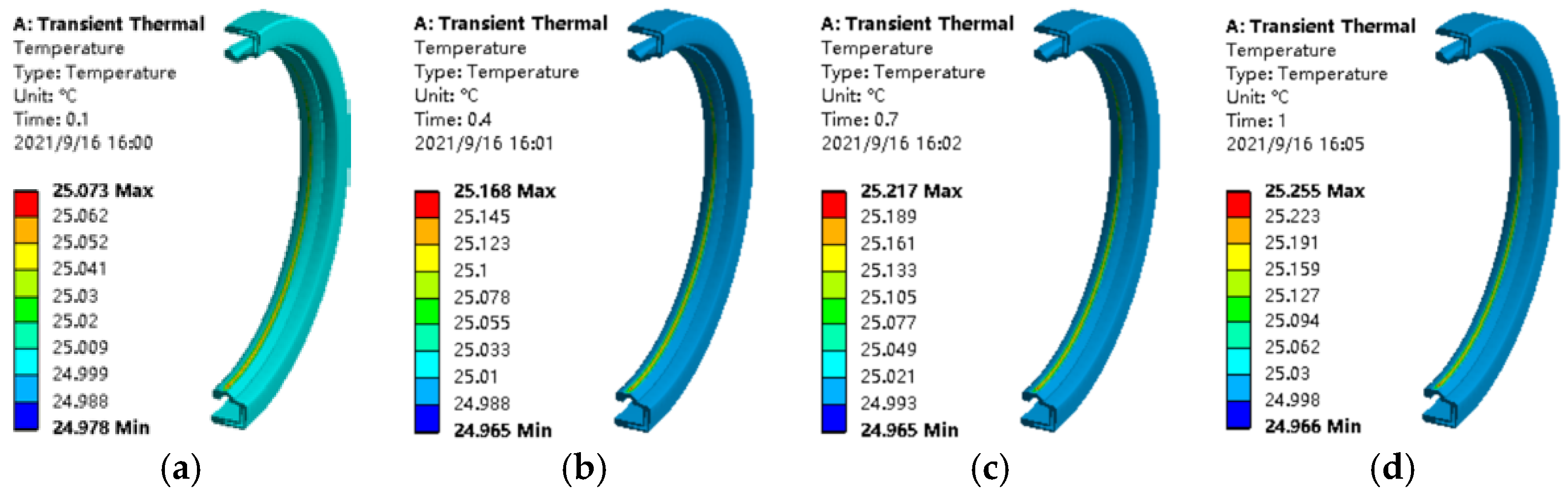
The total deformation of the AFHM when SEF = 25% is shown in Figure 16. The FE model of the dynamic seal can be built based on the nodal coordinates on the deformed profile of the AFHM. The contacting region distributes unevenly due to deflection of the axes between the stator and rotor. The contacting pressure distribution of the dynamic seal when SEF = 25% is shown in Figure 17. The maximum contacting pressure is 0.05 MPa. A transient thermal FE model of the dynamic seal is built. Both boundary conditions and initial conditions are set as introduced previously. The distribution of the temperature at different times is displayed in Figure 18.

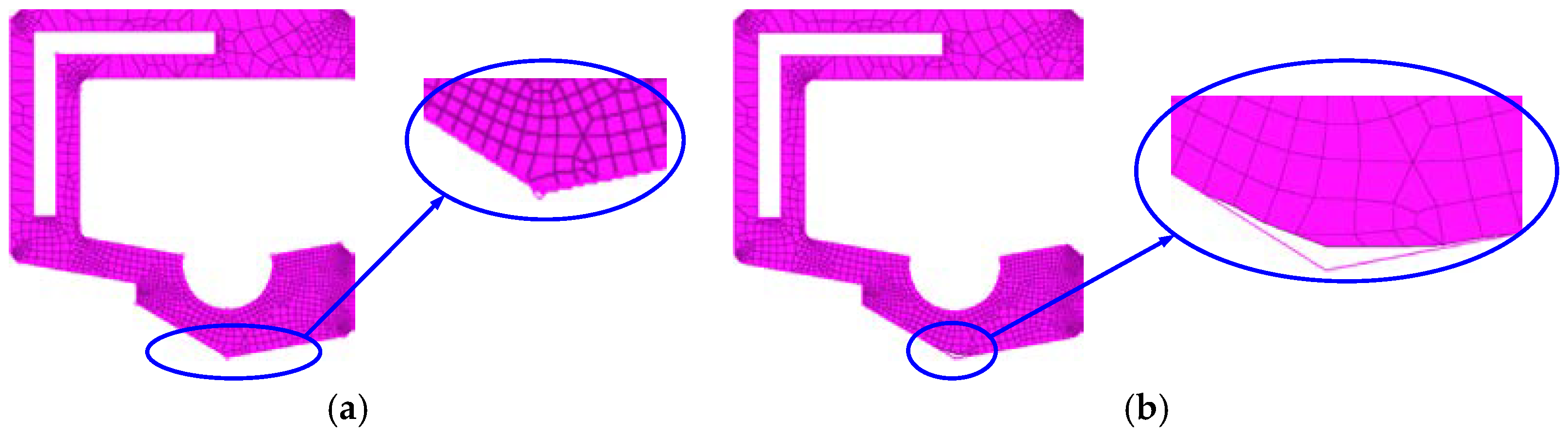
The worn effect of the dynamic seal for some periods is plotted in Figure 19. One section of the seal is shown in this figure. We can see the difference between the worn profiles and the unworn profile. Since the profile of the seal is changed, the contacting pressure will surely be affected. Thus, the influence of wear on the seal will be reflected with a change in the contacting pressure.

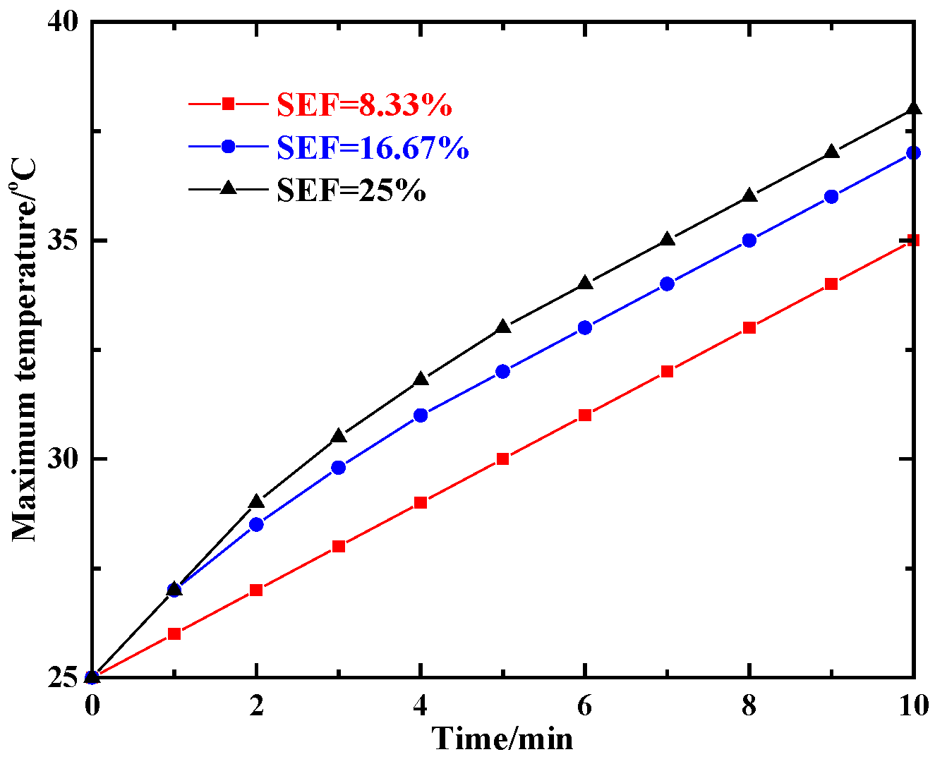
Variation in the maximum contacting temperature with time is plotted in Figure 20. It can be found from the results that as the deflection angle is increased, the temperature varies obviously in the first 2 min. This is caused by the uneven contact between the dynamic seal and stator. The uneven contact is more serious if the axes deflect more obviously. Thus the local contacting pressure reaches a larger value. Friction heat will have a more remarkable effect on making the seal expansion. However as wear goes on, the effect of uneven contact is reduced. The maximum contacting pressure is decreased and the variation gradient of the temperature is cut down. Therefore, we can see from the figure that temperature in the later period almost varies linearly.

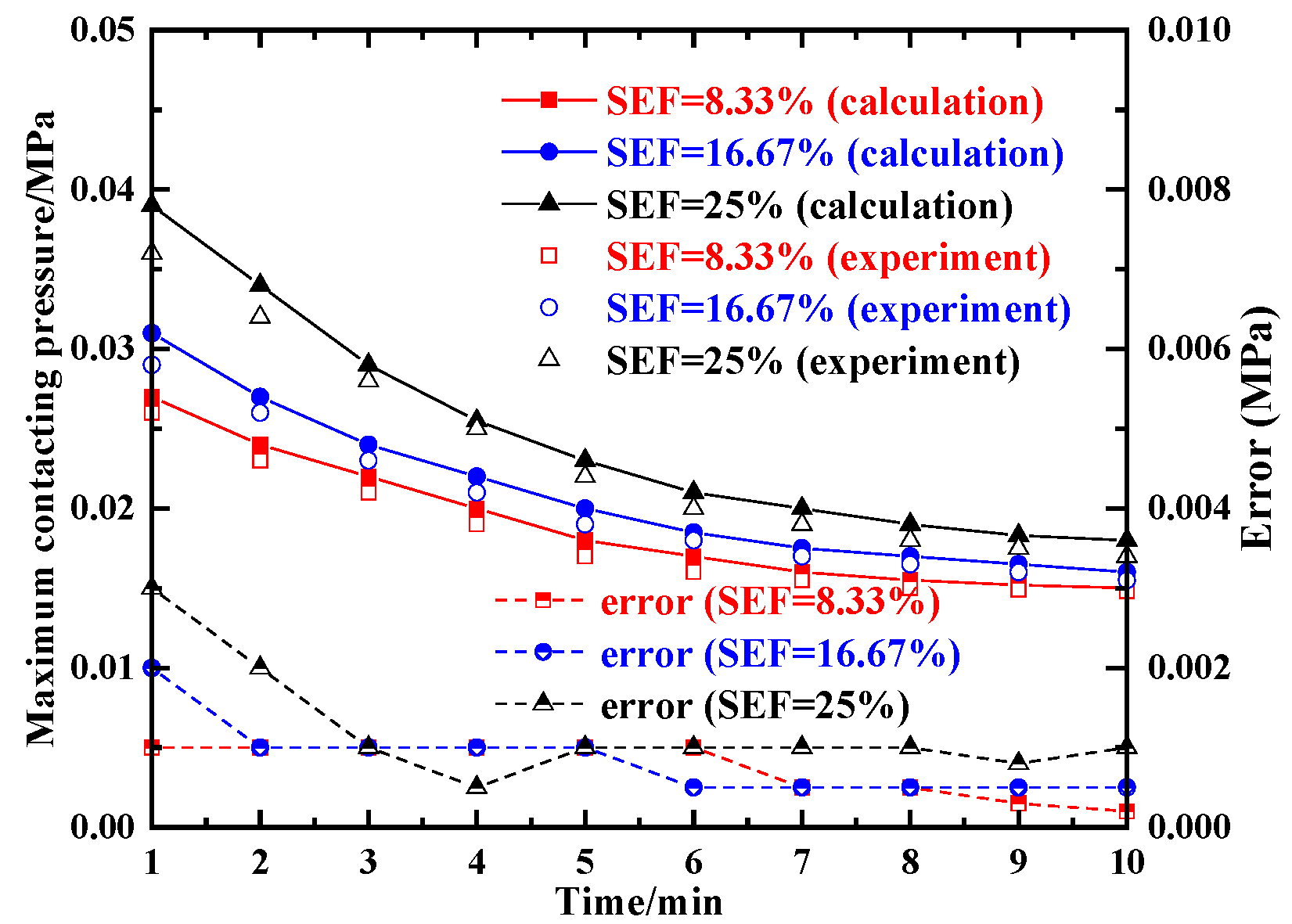
The variation in the maximum contacting pressure with time is displayed in Figure 21. We find that the maximum contacting pressure is increased as the deflection angle rises. However, as motor rotates at a high speed, the seal surface with a bigger contacting pressure is worn faster. Thus, on the curve representing a bigger deflection angle, the variation gradient of the maximum contacting pressure is more remarkable in the early period. Since the seal material is removed gradually, the contacting pressure is reduced. The wearing speed reduces lower, and then the variation speed of the maximum contacting pressure is also decreased. Thus, the curves become smooth in the later period. The dynamic seals in the experiment are dismounted after a specific period. Their FE models can be built based on the measured profiles. The maximum contacting pressure can be modeled. Thus the maximum contacting pressures at different times form the experimental results. We find that the experimental result is in accordance with the calculation results. The errors between the calculation results and the experimental results are also displayed. It is suggested that the error is bigger in the initial period. That is because the friction heat is not obvious in the initial period. Thus the thermal expansion does not affect the maximum contacting pressure significantly. In addition, the heat dissipation effect of the experiment is better than the proposed model (such as air conduction, which is not contained in the FE model). Although its effect is small, the influence can be reflected when the effect of friction heat is also small. As time goes by, the friction heat effect is more and more obvious. The weak heat dissipation can be ignored. The errors become small in the later period. Since the experimental results are obtained through measuring the profile of the dynamic seal under a disassembling state, the thermal expansion effect cannot be measured. Therefore, the experimental results are always smaller than the calculation results. It is proved that the presented method in this work is feasible.

6. Conclusions

A method of wear simulation for a dynamic seal in an AFHM is proposed in this work. A quasi-3D magnetic model of an AFHM without axes deflection is built. Then, the cogging effect is considered and an analytical model of UMF when axes deflection is taken into consideration is given. Boundary conditions of the FE model for a dynamic seal are obtained through solving the FE model of an AFHM. To consider the effect of friction heat on the wear of the seal, both structural and thermal FE models of the dynamic seal are presented. The structural–thermal coupled method is displayed. With the technology of mesh reconstruction proposed by the author previously, the dynamic simulation method for the wear of a dynamic seal is presented. The results display the influence of axes deflection on the distribution of the magnetic field in the air gap. The distribution of temperature in the dynamic seal field as well as the worn effect at different times is plotted. In the end, the variation in the maximum temperature and the maximum contacting pressure with time is presented. The experimental result proves that the method proposed in this work is feasible.