Article

Understanding the Influences of Multiscale Waviness on the Elastohydrodynamic Lubrication Performance, Part I: The Full-Film Condition

1
School of Mechanical Engineering and Automation, Harbin Institute of Technology, Shenzhen 518055, China
2
Institute of Functional Surfaces, School of Mechanical Engineering, University of Leeds, Leeds LS2 9JT, UK
*
Author to whom correspondence should be addressed.
Lubricants 2022, 10(12), 368; https://doi.org/10.3390/lubricants10120368
Submission received: 24 November 2022 / Revised: 14 December 2022 / Accepted: 15 December 2022 / Published: 18 December 2022
(This article belongs to the Special Issue Sustainable Elastohydrodynamic Lubrication)

Abstract

:
Understanding the responses of tribosystems to multiscale roughness is fundamental for the identification of the relevant roughness scales. This work used a point-contact elastohydrodynamic lubrication (EHL) problem as a representative tribosystem and artificially generated waviness with different amplitudes, frequencies, and directions to mimic the multiscale roughness. The amplitudes and frequencies are related to the feature geometry of smooth EHL problems. This work consists of Part I (this paper), focusing on the full-film condition, and Part II, focusing on the partial-film condition. Generated waviness is input to a transient thermal EHL model. The simulation is conducted 1600 times for different waviness parameters, loads, and speeds. Seven performance parameters are extracted: the minimum film thickness, maximum pressure, central film thickness, central pressure, mean film thickness, coefficient of friction (COF), and maximum temperature rise. The ratios of these parameters with and without waviness are plotted on the frequency–amplitude coordinate plane as contour maps. The influences of the amplitude, frequency, wave direction, load, and speed on the seven performance parameters are analyzed and summarized. The simulated data and plotted contour maps are provided to the readers in the Supplementary Material.

1. Introduction

Surface roughness is essential for modeling most tribology systems [1]. Modeling dry and lubricated contact between rough surfaces is key for understanding many tribological mechanisms, such as friction [2,3], adhesion [4,5], mixed lubrication [6,7], contact stiffness [8,9], and tribochemistry [10]. One fundamental issue of the modeling processes is the realistic representation of the roughness.
In 1957, Archard [11] first represented surface roughness through spherical protuberances of different length scales. Whitehouse and Archard [12] analyzed surface roughness using random process theories and recognized the multiscale features. Later, Sayles and Thomas [13] first utilized the nonstationary random process to characterize the multiscale properties of several engineering surfaces. However, the development of studies on nonstationary roughness was delayed following the pioneering work of Nayak [14] on stationary roughness following the steps of Longuet-Higgins [15]. By neglecting the influences of scales, stationary roughness is easier to analyze and use in modeling tribology systems. However, this does not mean that one can forget the importance of roughness scales. One fundamental question must be kept in mind: how does one select the appropriate roughness scales relevant to specific tribology systems?
Answering this question has significant theoretical and application value for the study of tribology systems. It could help us to understand further how surface roughness influences tribological performance. Moreover, based on the appropriate scales identified, modelers can use roughness data including all the essential features but excluding scales that are too fine to save computational resources. Furthermore, it can guide the industry to optimize the evaluation method for the surface topography, considering the fact that the finer the scale used for measurement is, the more expensive the measurement will be. Measuring the surface topography of parts on the relevant scales can help the industry to reduce costs and save time. Finally, knowledge about the influences of different roughness scales on tribology systems can help us to design functional multiscale surfaces. Customized multiscale surfaces could provide a way of enabling sustainable tribology systems. For example, EHL contacts could achieve a lower friction and longer service life with specially designed multiscale surfaces. In the meantime, if the multiscale surface is affordable for manufacturing, it can improve the sustainability of many technical applications, such as the gears and bearings, which include EHL contacts.
Progress in the study of nonstationary roughness sheds some light on the answer to the question posed above. Nonstationary roughness regained attention after the rapid development of fractal concepts in the 1980s [16]. The extraordinary advantage of fractal concepts is that they can provide scale-invariant parameters, e.g., the fractal dimension, to characterize multiscale geometries. Majumdar and Bhushan [17] first employed scale-invariant fractal methods to characterize the nonstationary roughness. The use of fractal methods promotes the study of the dry contact between rough surfaces [18,19,20,21]. Based on these models, the relationship between roughness scales and tribological quantities can be investigated. It has been found that some quantities, such as the real contact area and rubber friction dissipation, are principally related to the high-frequency parts of the surface roughness [22]. Meanwhile, other quantities, e.g., the stiffness and electrical conductance, are more relevant to the low-frequency contents [23,24]. These findings prove that surface roughness, on specific scales, is more relevant to specific quantities in dry contact with rough surfaces.
Unlike its extensive applications in dry contact analysis, multiscale roughness is seldom discussed in regard to the modeling of lubricated contact, although lubricated contact models considering roughness have been studied for more than 50 years. One breakthrough work was the development of the average-flow Reynolds equation theory by Patir and Cheng [25,26,27]. They introduced correction coefficients, named flow factors, in the well-known Reynolds equation to statistically incorporate the assessment of the effect of roughness on lubrication performance. Following this concept, a more general and unambiguous approach, the homogenization technique, was used to calculate more comprehensive and accurate flow factors [28,29,30,31,32]. Some researchers [33,34,35] developed double-scale solvers for lubricated contact. Although different theories, equations, and algorithms are used in these methods, they have one point in common: a relatively small-scale calculation domain is required to incorporate the stationary surface textures. However, researchers have seldom discussed the criteria for selecting the small-scale calculation domain from the tribology system perspective.
In addition to the stochastic models mentioned above, researchers [7,36,37,38,39,40,41,42,43,44] have also directly used simulated or measured deterministic roughness data for solving the Reynolds equation, especially in the analysis of elastohydrodynamic lubrication (EHL). Although most work ignores the multiscale characteristic of roughness, some researchers have noted this problem. Demirci et al. [39] deconstructed the measured roughness on different scales and predicted the scale effect on the mixed-point-contact EHL performance. They concluded that finer (smaller) scales could result in a smaller friction coefficient. Zhang et al. [7] studied the influences of fractal surfaces on the load-carrying capacity of a thrust bearing. The results showed that the high cut-off frequency of the fractal roughness significantly influenced the load-carrying capacity. Li and Yang [43] analyzed the effects of fractal surfaces on point-contact EHL, but they did not discuss the impacts of the scales on the EHL performance.
In summary, few studies have paid attention to the multiscale characteristic of roughness for lubricated contact with roughness, whether the roughness is used statistically or deterministically. Thus, the essential question of which roughness scales are relevant to a specific lubricated contact problem is still unclear and requires further study.
In order to investigate this question, the responses of specific lubricated contacts to multiscale roughness should be understood first. In real-world applications, lubricated contacts take various forms, such as ball bearings, gears, sliding bearings, and mechanical seals. Different forms have particular features and performances of interest, resulting in complexity when studying their responses to multiscale roughness. To avoid such complexities, we selected the point-contact elastohydrodynamic lubrication (EHL) problem as a representative research object, because it can describe the fundamental physics of many lubricated contacts and has been well modeled by researchers.
After selecting the point-contact EHL problem, the multiscale roughness should also be specified. However, using specific simulated or measured rough surfaces will limit the obtained responses of the EHL system to multiscale roughness with respect to the surfaces used. Such case studies cannot help us to obtain a relatively comprehensive image of how an EHL system responds to multiscale roughnesses or inspire methodologies that can be used to identify relevant roughness scales. Thus, a general way of representing the features of multiscale roughness, regardless of any specific roughness, should be used.
It is known that a multiscale roughness can be represented as the summation of the roughness components within different frequency bands (scales). Each roughness component has a different amplitude. Thus, a scale-limited roughness component can be represented by two essential features: the frequency and amplitude. Such a phenomenon indicates that designing a series of single-scale wavy surfaces provides a way to mimic the scale-limited roughness components. Venner and Lubrecht [45] also used a series of single-scale waviness to mimic the multiscale roughness.
These single-scale wavy surfaces are not relevant to any specific multiscale roughness. One can use them as inputs to simulate the EHL system. The corresponding results can be regarded as a reference that is not limited to a specific multiscale roughness, indicating the comprehensive and standard responses of the EHL system to roughness components of different frequencies and amplitudes. Therefore, artificially generated wavy surfaces are used in the current research to mimic the multiscale roughness. In addition to the amplitude and frequency, the other important parameter, the direction of the waviness, is also considered as a variable in the generation of different wavy surfaces.
In summary, the current study explores the influence of multiscale waviness on the point-contact EHL problem. The results provide a relatively general and comprehensive understanding of the responses of the EHL system to multiscale roughness, which could inspire the further development of new methodologies to identify roughness scales that are relevant to the studied EHL system. Moreover, the methodologies could be transferred to study other kinds of tribosystems. The EHL system can work in either full-film or partial-film conditions. Having both full and partial film EHL results in one paper will be lengthy. Therefore, the current research will be reported in a two-part series of papers. This paper, part one, focuses on discussing the results under full-film conditions. The partial-film results will be published in part two.
The detailed organization of this article is as follows. First, the theories and methods are introduced, including the computation model section and wavy surface generation section. The validation of the models is provided in the Supplementary Material. Then, the configuration of the numerical simulations is provided in detail. Finally, the simulation results are analyzed and discussed.

2. Materials and Methods

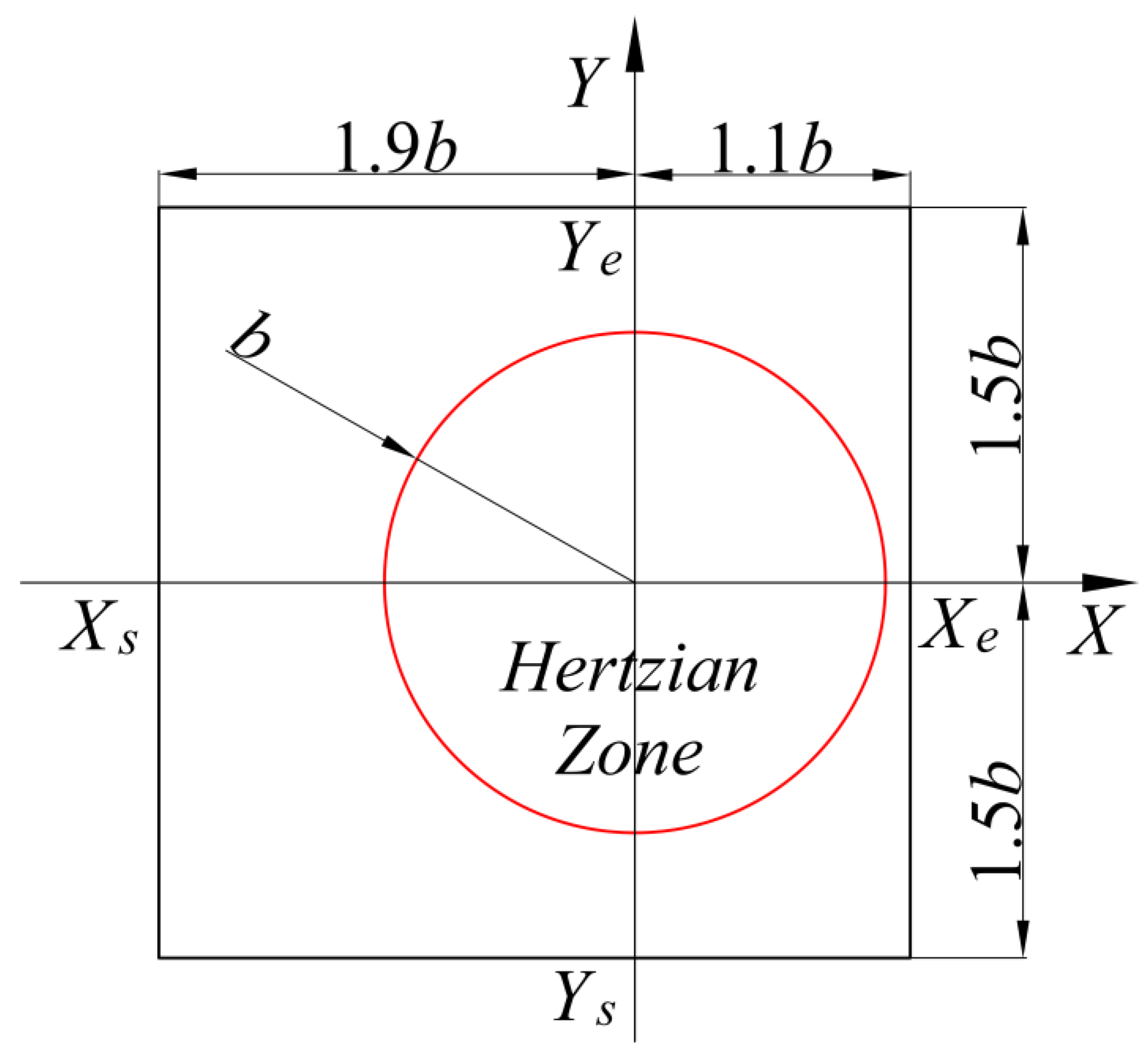
2.1. Computation Model

A transient thermal EHL model (TEHL) was used in the current research. This model can also predict the coefficient of friction (COF). As the TEHL model has been extensively reported in the literature, only some key features of the computation model are clarified in this section. The viscosity–pressure–temperature relationship is considered by combining the Barus viscosity–pressure and Reynolds viscosity–temperature equations. The density–pressure–temperature relationship is considered using the Dowson–Higginson equation. When solving the Reynolds equation, the lubricant is assumed to be Newtonian. When calculating the shear stress, a non-Newtonian behavior is considered based on the shear stress model reported by Bair et al. [46]. The detailed equations, numerical solution procedures, and validations are provided in Supplementary Material S1. Interested readers can also refer to the authors’ previous work [47] and other literature [48].
Figure 1 shows the solution domain, whose coordinate system is defined according to the Hertzian contact zone. The coordinate origin is at the center of the Hertzian contact zone, and the X-direction represents the relative motion direction between the two mating surfaces. The Y-direction is perpendicular to the X-axis. The solution domain is square, with a side length equal to three times the radius of the Hertzian contact zone, b. According to the non-dimensionalization procedures (see Supplementary Material S1), the non-dimensional solution domain is Xs ≤ X ≤ Xe and Ys ≤Y ≤Ye, where Xs = −1.9, Xe = 1.1, Ys = −1.5, and Ye = 1.5. This size of the solution domain has been widely used in the literature to analyze EHL problems [42,49,50]. This solution domain is discretized into M × N grids, where M = N = 256. In particular, M is the number of grids in the X-direction.

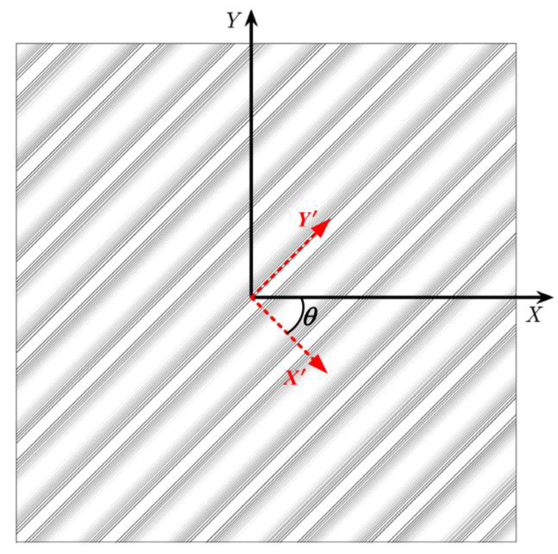
2.2. Wavy Surface Generation

According to the literature [51,52], a general wavy surface has three key parameters: the amplitude, wavelength, and direction. Figure 2 shows a wavy surface with an arbitrary direction angle θ, which is the angle between the relative motion direction, X, and the wave direction, X′. When θ = 0°, it represents the transverse waviness. In the case of θ = −90°, longitudinal waviness is generated. The equation for generating waviness, rθ, is modified from Venner and Lubrecht, given in Equation (1) [51]:
r θ ( X , Y , t ¯ ) = a x cos [ 2 π ( X X d ) Λ x ]
a x = { a × 10 10 [ ( X X d ) / Λ x ] 2 ,   if   X X d > 0 a ,   otherwise
where a is the dimensional amplitude, Λx is the non-dimensional wavelength, and the corresponding non-dimensional frequency is Ωx = 2π/Λx. The amplitude a is modulated to ax to initiate the waviness with continuous derivatives using Equation (2) [51]. Xd is the location of the start of the waviness, and its value changes as the non-dimensional time t ¯ increases, as calculated using Equation (3) [51]:
X d = X s + cos ( θ ) 2 t ¯ u 2 u s
where us = u1 + u2 is the sum of the velocities of the two surfaces, and u2 is the velocity of the wavy surface. X s is the start of waviness at t ¯ = 0 with the wave direction θ, which is calculated using the following equations:
[ X s Y s   ] = { M ( θ ) [ X s Y e ] ,   if   θ 0 M ( θ ) [ X s Y s ] ,   if   θ > 0  
where M (θ) is the rotation matrix:
M ( θ ) = [ cos ( θ ) sin ( θ ) sin ( θ ) cos ( θ ) ]
Theoretically, the amplitude and wavelength values can be selected arbitrarily. However, bearing in mind that the ultimate purpose of this research is to identify relevant roughness scales for EHL problems, linking their values with specific EHL conditions is a better option. The specific EHL conditions are the working conditions of the EHL systems of interest with smooth surfaces. Thus, in this work, we set the amplitude and frequency values based on the critical features of an EHL problem. The amplitude, a, is linked with the central film thickness of the smooth EHL problem whose working parameters are the same as those of the EHL problem with wavy surfaces, resulting in the equation:
a = A h c e n t s
Where A is defined as the non-dimensional amplitude, and h c e n t s represents the central film thickness with the smooth surface.
The wavelength, Λx, is linked with the radius of the nominal Hertzian contact zone, b (see Figure 1). In order to further simplify the setting of the wavelength value, the number of waves in the solution domain, Nw, is used to calculate the non-dimensional wavelength, Λx, as follows:
Λ x = X e X s N w
Then, the non-dimensional frequency, Ωx, is calculated as follows:
Ω x = 2 π Λ x = 2 π N w X e X s = 2 π N w 3
The specific values of A and Nw are provided in Section 2.3. It should be noted that the Ωx is proportional to the Nw and inversely proportional to the X e X s . Using Equations (6)–(8), the amplitude and frequency values are defined based on the performance parameters of the smooth EHL problems. In doing so, a relatively standardized reference system can be established to evaluate the influence of the waviness on the EHL performance. This reference system can avoid the unwanted distortion of dimensional waviness during the non-dimensionalization procedures when the working condition changes.

2.3. Numerical Simulation Details

The codes used in the current work are verified by the experimental results of He et al. [48]. Detailed verification results are provided in Supplementary Material S1 (Figure S2). The basic parameters of the EHL simulation are also from the same work, listed in Table 1 [48]. It should be noted that the disk and ball are formed of steel. The selected thermal conductivity (46 W m−1∙K−1 in Table 1) is reported to correspond to that of steel in its annealed, soft state [53]. Hardened steel has a thermal conductivity of approximately 21 W m−1∙K−1 [53]. Such a difference in thermal conductivity has been proven to lead to the overestimation of the friction under the conditions of a high slide-to-roll ratio (SRR) [54,55]. The SRR used in this work is −0.2 (Table 1), close to the pure-rolling condition (SRR = 0). Therefore, the thermal conductivity value of steel (46 W m−1∙K−1) widely used in the literature is also used in the current work. One should pay attention to the thermal conductivity of the steel if relatively high SRRs are studied.
In order to test various working conditions, two load values, w = 200 N and 500 N, and two speeds, us = 0.3 m/s and 3 m/s, were used in the simulations. It should be noted that full-film EHL conditions are obtained with these parameters. The central and minimum film thicknesses are listed in Table 2. Table 2 also lists the other five key performance parameters of the four working conditions without waviness: the mean film thickness, central pressure, maximum pressure, coefficient of friction (COF), and maximum temperature rise.
The amplitude and frequency values used in this work were calculated based on Section 2.2 for each group of load and speed conditions. The non-dimensional amplitude, A, was set to be equal to 0.02, 0.027, 0.037, 0.049, 0.067, 0.09, 0.122, 0.164, 0.222, and 0.3. The frequency values were only a function of Nw, according to Equation (8). The Nw values used were 2, 6, 9, 12, 16, 19, 22, 25, 29, and 32. The grid convergence study was conducted for the largest Nw value, Nw = 32. The results show that the grid size of 256 × 256 is sufficient to obtain results of an acceptable accuracy (see Figure S5 in Supplementary Material S1). According to Equation (8), the corresponding Ωx values were approximately 4, 13, 19, 25, 33, 40, 46, 52, 61, and 67. It should be noted that the Ωx value changes when using a different solution domain size ( X e X s ). The current work selected the minimum one ( X e X s = 3 ) from among the sizes of the solution domain that can be found in the literature, e.g., X e X s = 3 [42,49,50], 4 [56], 5.5 [44], or 7 [43]. Because the Nw value is the maximum when considering the grid convergency and computational efficiency (for example, 32 in this work), a relatively small X e X s value can increase the upper limit of the Ωx value (see Equation (8)).
The selection of the wave directions is meant to include the transverse (θ = 0°), longitudinal (θ = −90°), and several intermediate directions. The current work used −30° and −60° as the intermediate wave directions to balance the computational cost and parameter diversity. Thus, each group of amplitude and frequency conditions were used to simulate wavy surfaces with four different wave directions, which were θ = 0°, −30°, −60°, and −90°, representing the rotation of the waviness from transverse to longitudinal.
The time interval of the simulation, Δ t ¯ , is set to the value that is equal to the shifting of the wavy surface by the distance of one grid, calculated as follows:
Δ t ¯ = u s ( X e X s ) 2 u 2 ( M 1 )
This means that at each time step, the entire wavy surface moves the distance of one grid in the X-direction. The time step for the termination of the simulation, NT, is set as NT = 3 × M = 768 to obtain a stable solution to the transient EHL problem. The simulation results (see Supplementary Material S1, Figures S3 and S4) show that this NT value is sufficient to obtain a stable solution to the transient EHL problem. Another point to note is that the different load, speed, amplitude, and frequency values are designed to maintain the corresponding EHL problems in the full-film regime. The simulations were run on the ARC3, part of the High-Performance Computing facilities at the University of Leeds, UK, with E5-2650v4 CPU, 2.2 GHz. The CPU time varies from a dozen to 50 h for different combinations of the waviness parameters, load, and speeds. We took advantage of the High-Performance Computing facilities by running tens of programs with different parameter combinations simultaneously.
Based on the transient simulation results, seven critical performance parameters were extracted to characterize the responses: the minimum film thickness, maximum pressure, central film thickness, central pressure, mean film thickness, maximum temperature rise, and coefficient of friction (COF). In the transient simulation, these parameters change as the time step increases. Even if the transient solution is stable, small fluctuations still exist (see Figures S3 and S4 in Supplementary Material S1). Therefore, to obtain representative performance parameter values, they should be averaged over the time in which the transient solution is stable. The time steps used to obtain the average were set as the last surface movement period. Because the wavy surface circulates as the length of time increases, the parameter fluctuations adopt the same period. Adopting the last surface movement period can ensure that an entire period of parameter variations is extracted from the stable transient solution.

3. Results and Discussion

The ratios of the performance parameters with and without waviness were calculated and plotted as contour maps on the frequency–amplitude (Ωx − Ax) coordinate plane with the double logarithm scale to highlight the influence of wavy surfaces on the EHL performance. The contour lines are labeled with their values in most cases. Some contour lines are not labeled due to the lack of drawing space. In order to ensure the brevity and clarity of this article, only representative plots are shown in this section. All the plots and the simulation data used to plot them are included in the Supplementary Material S2.

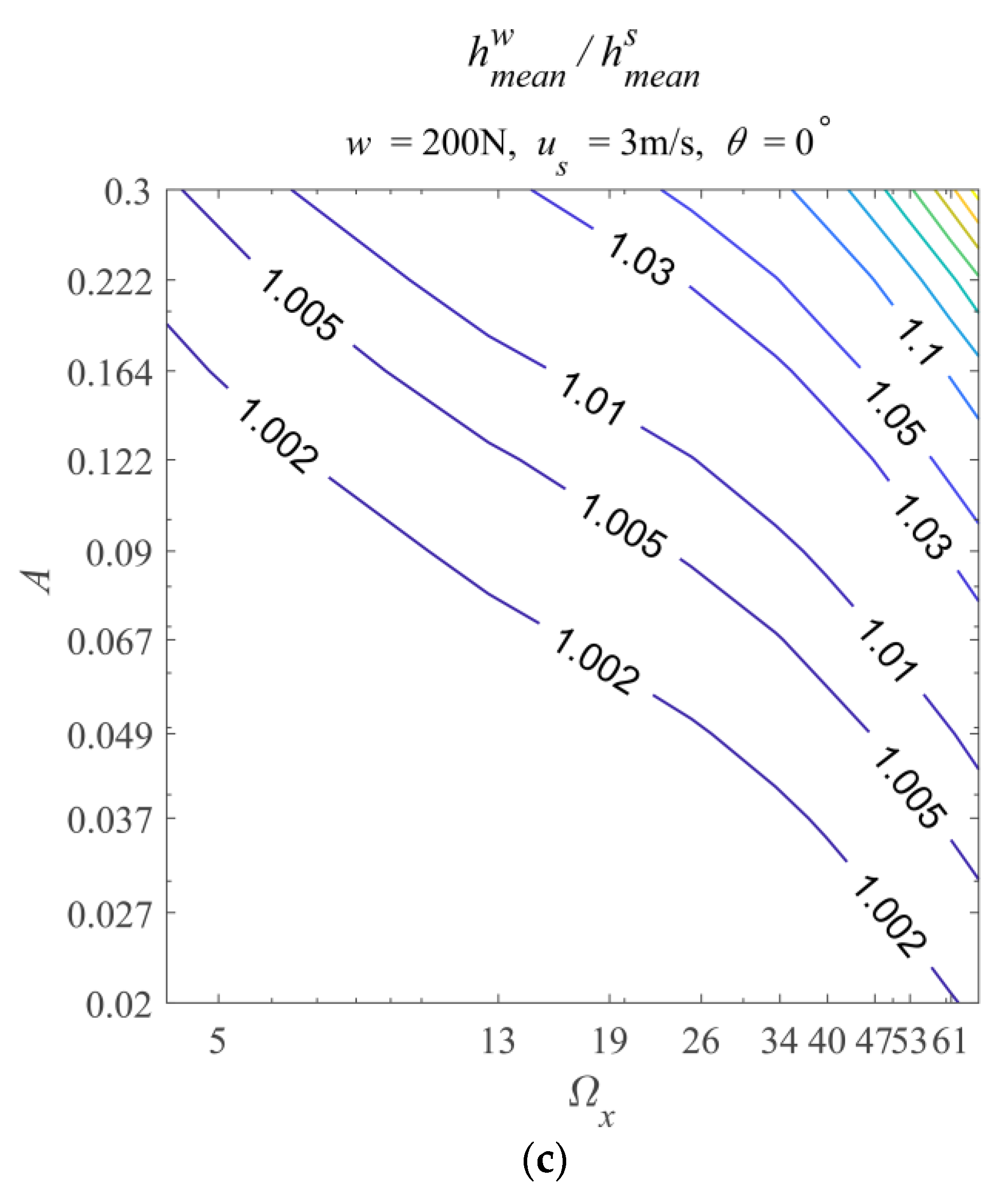
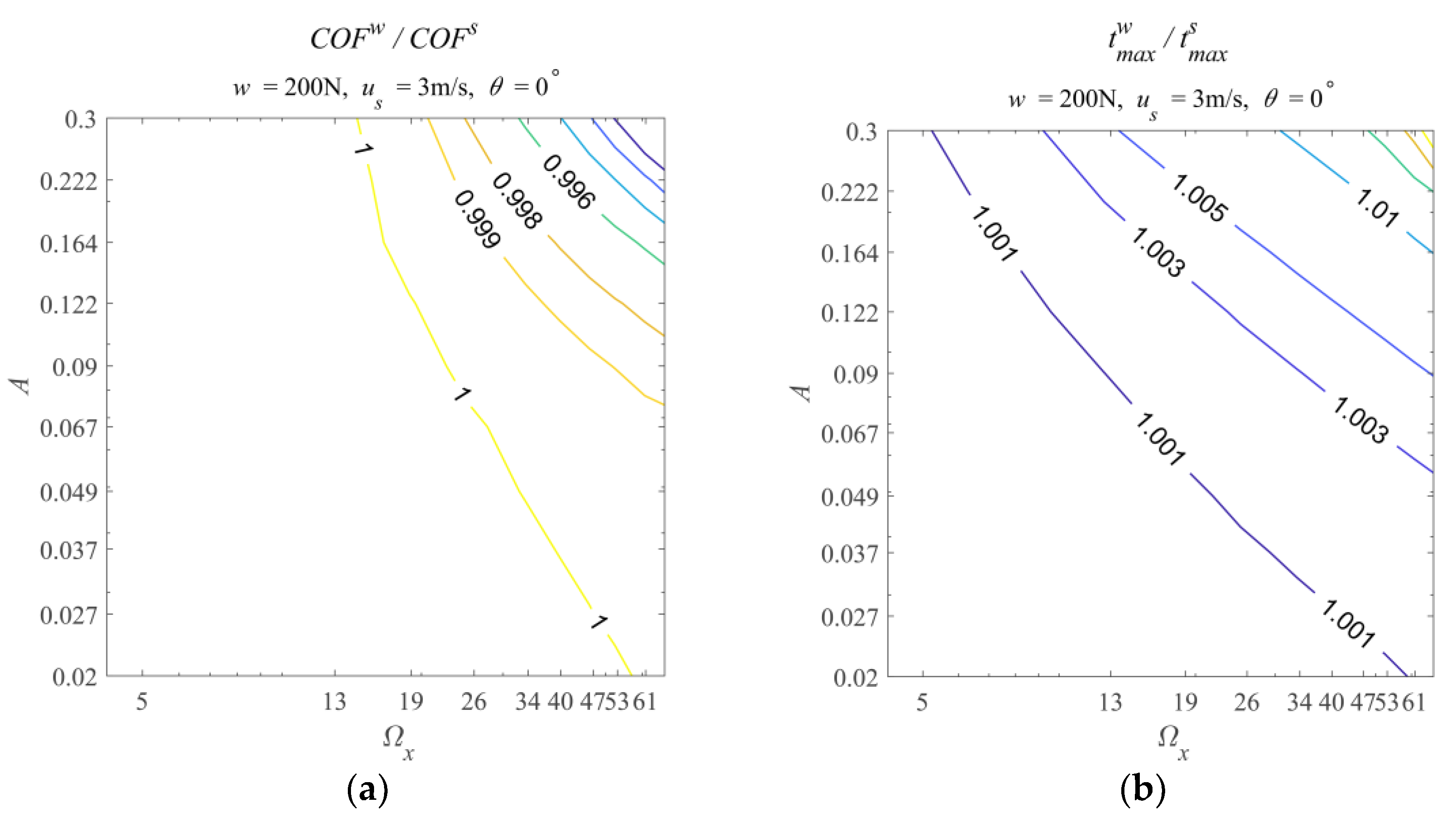
3.1. The Influences of the Waviness Amplitude and Frequency

Without the loss of generality, the results simulated with w = 200 N, us = 3 m/s, and θ = 0° are discussed in this section to illustrate the influences of the waviness amplitude and frequency for the sake of brevity. Figure 3, Figure 4 and Figure 5 show the contour maps, and Table 3 lists the corresponding range of the ratios of the performance parameters rounded to three decimal places.
Figure 3a–c shows the contour maps related to the film thickness parameters. In Figure 3a, the h min w / h min s ratios are less than one in most cases, indicating that the minimal film thickness is reduced when waviness is incorporated. Venner and Lubrecht [51] and Ehret et al. [52] also reported the reduction in the minimal film thickness when a transverse waviness (θ = 0°) was incorporated into the point EHL. As the A and Ωx increase, the h min w / h min s ratio changes nonmonotonically. When the Ωx value is relatively small (Ωx < 30), increasing A or Ωx decreases the h min w / h min s ratio. With the further increase in the Ωx value, the h min w / h min s ratio gradually increases. The Ωx value of the inflection point differs from the A value used. With a larger A value, the Ωx value of the inflection point is larger.
When Ωx ≈ 30 and A = 0.3, the h min w / h min s ratio reaches a minimum value of around 0.772 (Table 3). This value is not explicitly shown in the contour map due to the lack of drawing space available to add contour line labels. Instead, it is estimated from the simulated dataset (see Supplemental Material S2). The same approach is used below. One should note that this estimation of the minimum point is based on specific simulation conditions. Such a minimum point suggests that a specific combination of the amplitude, frequency, and direction of waviness could result in the most significant reduction in the minimum film thickness. Based on the authors’ knowledge, this paper reports such phenomena for the first time.
Figure 3b shows that the h c e n t w / h c e n t s ratios are greater than one, indicating that the central film thickness is enhanced when waviness is incorporated. The h c e n t w / h c e n t s ratio increases as A or Ωx increases. Within the simulated ranges of A and Ωx, the maximum h c e n t w / h c e n t s value is around 1.451 (Table 3) when Ωx ≈ 67 and A = 0.3. This point is situated at the top right-hand corner of the contour map, which is the combination of the maximum frequency and maximum amplitude within the range of the simulation parameters. Such results indicate that increasing the amplitude or frequency leads to a thicker central film thickness than the value without waviness. Increasing the amplitude and frequency have synergistic effects in enhancing the central film thickness.
Figure 3c shows that the h m e a n w / h m e a n s contour map has the same trend as the h c e n t w / h c e n t s contour map in Figure 3b. The h m e a n w / h m e a n s ratios are greater than one and increase as A or Ωx increases. The maximum h m e a n w / h m e a n s value is approximately 1.423 (Table 3), occurring at the point of Ωx ≈ 67 and A = 0.3. Such results suggest that the mean film thickness is enhanced by waviness. The magnitude of this enhancement can be increased by increasing either the amplitude or the frequency. Increasing the amplitude and frequency have synergistic effects in enhancing the mean film thickness. Venner and Lubrecht [51] and Ehret et al. [52] also reported the enhancement of the central and mean film thickness by waviness, although they only used a certain number of amplitudes and frequencies.
Combining Figure 3a–c, it can be concluded that the waviness increases the central and mean film thickness but decreases the minimum film thickness at the same time. The central film thickness is the film thickness at the fixed central point ( X = 0 , Y = 0 ) in the solution domain. The mean film thickness is the average value of the film thickness values within the nominal Hertzian contact zone. The increase in the central and mean film thickness proves that incorporating waviness can further lift the ball, representing a kind of enhancement of the EHL effect. As the name suggests, the minimum film thickness is the minimum value of the film thickness distribution. The decreased minimum film thickness indicates that the lifting effect of the ball is inadequate to counteract the effects of the wave valleys on the minimum film thickness. The decrease in the minimum film thickness is usually considered to be a degradation of the EHL performance.
Furthermore, the central and mean film thicknesses are increased most with the maximum frequency (Ωx ≈ 67) and maximum amplitude (A = 0.3) within the range of simulation parameters. At this point, the h min w / h min s ratio is almost equal to one (around 0.974, see Supplementary Material S2), indicating a very small reduction in the minimum film thickness. Therefore, the point (Ωx ≈ 67, A = 0.3) is the best choice within the range of simulation parameters, which can be considered to enhance the EHL effect in terms of the film thickness, with w = 200 N, us = 3 m/s, and θ = 0°.
Figure 4a,b shows the ratios of the maximum pressure with and without waviness ( P max w / P max s ) and the ratios of the central pressure with and without waviness ( P c e n t w / P c e n t s ), respectively. Figure 4a shows that the P max w / P max s ratios are greater than one, indicating that incorporating waviness results in a more significant maximum pressure. When the A or Ωx increases, the P max w / P max s ratio increases. The maximum P max w / P max s value is approximately 2.042, again occurring at the point of Ωx ≈ 67 and A = 0.3. Such results suggest that increasing the amplitude or frequency results in a higher maximum pressure. Simultaneously, increasing them has synergistic effects in enhancing the maximum pressure. Combining Figure 3a–c and Figure 4a, waviness with a high frequency and large amplitude can generate a thicker lubricant film in terms of the central and mean film thickness, but this is accompanied by a larger maximum pressure. For example, at the point of Ωx ≈ 67 and A = 0.3, the h m e a n w / h m e a n s value is approximately 1.423, and the P max w / P max s value is approximately 2.042. The maximum pressure increase is usually considered negative in an EHL system. Thus, it is necessary to comprehensively consider the influences of waviness on the film thickness and pressure when one wishes to utilize waviness to enhance the EHL effects.
Figure 4b shows that the P c e n t w / P c e n t s results are very different from the P max w / P max s results. Most of the P c e n t w / P c e n t s ratios are around one. The P c e n t w / P c e n t s ratios fluctuate as the Ωx increases. Increasing A can slightly increase the P c e n t w / P c e n t s ratios. The P c e n t w / P c e n t s value is within the range of [0.998, 1.016]. Such results should be because the central pressure is the pressure at the fixed central point. The pressure value at the central point is more dominated by the maximum Hertzian contact pressure, which is a constant in a given EHL problem. In comparison, the P c e n t w / P c e n t s ratio contour map provides less information than the P max w / P max s ratio contour map.
Figure 5a,b shows the ratios of the COF with and without waviness ( C O F w / C O F s ) and the maximum temperature rise with and without waviness ( t max w / t max s ), respectively. Figure 5a shows that the C O F w / C O F s ratios are greater than one when the A and Ωx values are relatively small. The corresponding maximum value is approximately 1.001 (Table 3). As the A or Ωx values further increases, the C O F w / C O F s ratios gradually decrease and are smaller than one. The minimum C O F w / C O F s ratio is approximately 0.983, also occurring at Ωx ≈ 67 and A = 0.3. These results suggest that incorporating waviness can increase the COF, with relatively small amplitudes and frequencies, or decrease the COF, with relatively large amplitudes and frequencies.
Figure 5b shows that the t max w / t max s ratios are greater than one, indicating that incorporating waviness results in a higher temperature rise in the lubrication film. The t max w / t max s ratio increases as the A or Ωx increases. The maximum t max w / t max s ratio is approximately 1.030 when Ωx ≈ 67 and A = 0.3. These results indicate that increasing the amplitude and frequency synergistically increases the temperature rise in the lubrication film.
Combining Figure 5a,b, the reason why the COF drops could be the temperature rise with waviness. The temperature rise reduces the lubricant’s viscosity, resulting in shear stress reduction. He et al. [48] also reported the COF reduction as the increase in the film thickness based on experiments and simulations. They concluded that the main reason for this is the viscosity decrease resulting from the temperature rise. One aspect to note is that both the C O F w / C O F s and t max w / t max s ratios are close to one. The reason for this should be that the SRR used is −0.2 (Table 1), resulting in a small sliding velocity between the ball and the disc. The amount of generated frictional heat is small, resulting in a slight decrease in the lubricant’s viscosity, which leads to a slight decrease in the COF.
Combining the information in Figure 3, Figure 4 and Figure 5, waviness with a high frequency and large amplitude can generate a thicker lubricant film in terms of the mean and central film thickness, with a higher maximum pressure, and result in a smaller COF, with a higher temperature rise. In general, a thick lubricant film and small COF are positive results, but a high maximum pressure and temperature rise are negative when studying EHL problems. Incorporating waviness can affect them simultaneously. Thus, the conclusion as to whether waviness benefits or does not benefit an EHL problem cannot be drawn directly. After comprehensively considering these pros and cons, one may decide on whether incorporating waviness will benefit their specific studies.

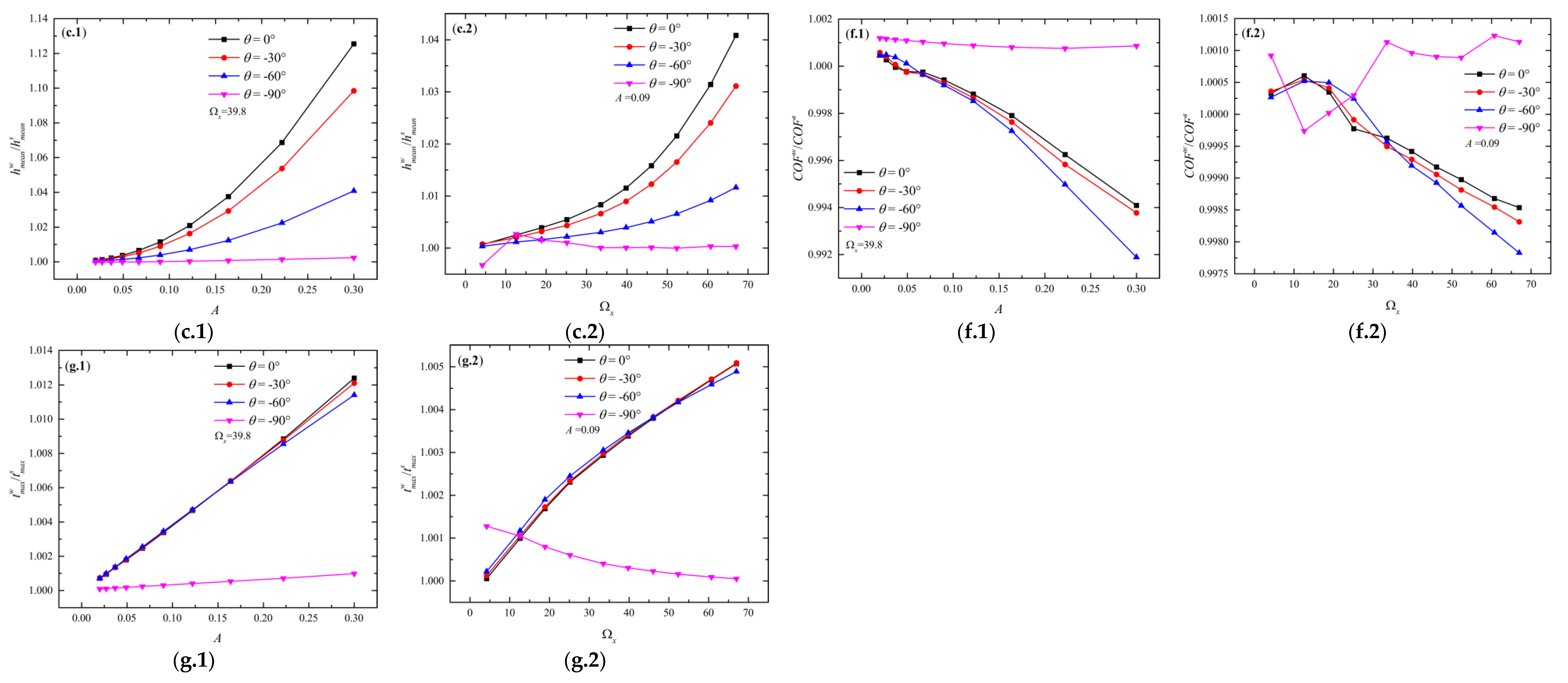
3.2. The Influence of the Wave Direction

The results simulated with w = 200 N and us = 3 m/s are used to discuss the influence of the wave direction. In order to highlight the influences of the wave directions, two cross lines of each contour map were extracted, which are the lines with fixed A = 0.09 or fixed Ωx ≈ 39.8 (Nw = 19). Then, the extracted lines with the same type of performance parameters were plotted in one graph. In each graph, the four curves correspond to the four directions θ = 0°, −30°, −60°, and −90°. There are fourteen such graphs, which are organized as sub-figures in Figure 6. Indices a to g represents the seven performance parameters, where ‘1’ and ‘2’ indicate the results of the fixed Ωx ≈ 39.8 and A = 0.09, respectively.
All the h min w / h min s ratios in Figure 6a.1 are smaller than one, indicating the minimum decrease in the film thickness due to waviness. Figure 6a.1 shows that the h min w / h min s ratio decreases for a large amplitude (approximately A > 0.05) when the wave direction turns from transverse (0°) to longitudinal (−90°). When the amplitude is small (approximately A < 0.05), the h min w / h min s ratios are almost invariant as changing wave directions.
Figure 6a.2 shows that the h min w / h min s ratios are smaller than one and decrease as the wave direction changes from 0° to −60°. Such a decrease becomes greater with higher frequencies. When the wave direction equals −90°, the h min w / h min s ratio shows a different pattern. It decreases with significant fluctuation as the Ωx increases. The h min w / h min s ratios with θ = −90° are even greater than one for some frequency values. For instance, h min w / h min s equals 1.003 when Ωx ≈ 19 and A = 0.09. This result indicates that the minimal film thickness can be increased by incorporating specifically designed longitudinal waviness.
Overall, with the exception of some special types of longitudinal waviness, converting the transverse waviness to longitudinal waviness decreases the h min w / h min s ratio under most circumstances. The results reported by Ehret et al. [52] also support this point.
Figure 6b.1 shows that the h c e n t w / h c e n t s ratios are greater than one and increase as the A increases when θ = 0°, −30°, and −60°. The h c e n t w / h c e n t s ratios decrease as the waviness transforms to become longitudinal, especially for large amplitudes. While θ = −90°, the h c e n t w / h c e n t s ratios quickly decrease as the A increases, suggesting that the longitudinal waviness decreases the central film thickness. Figure 6b.2 indicates the same patterns as Figure 6b.1. In general, converting the transverse waviness to longitudinal waviness decreases the h c e n t w / h c e n t s ratio.
Figure 6c.1,c.2 indicates that the h m e a n w / h m e a n s ratio also decreases as the waviness becomes longitudinal. In particular, for θ = −90°, the h m e a n w / h m e a n s ratio is approximately one as the amplitude and frequency vary. This means that longitudinal waviness has little effect on the mean film thickness. Combining Figure 6a–c, it can be concluded that converting transverse waviness to longitudinal waviness decreases the EHL effects in terms of the film thickness under most circumstances. The reason for this should be that converting the waviness from transverse to longitudinal decreases the waviness’s equivalent frequency in the direction of the relative motion (X-direction). The deviation in the surface geometry in the direction of the relative motion plays a critical role in generating hydrodynamic effects. According to the discussion in Section 3.1, the frequency decrease in the X-direction usually decreases the EHL effects in terms of the film thickness.
Figure 6d.1,d.2 shows that the P max w / P max s ratios are almost unaffected by the alterations in the wave directions among 0°, −30°, and −60°. The P max w / P max s ratios are greater than one and increase as the A or Ωx increases. When θ = −90°, the P max w / P max s ratios are still greater than one, but their increase with the increasing A or Ωx is far slower than those of the other wave directions. These results indicate that the maximum pressure is increased once waviness is incorporated. Among the different wave directions, the longitudinal waviness produces the slightest increase in the maximum pressure.
Figure 6e.1,e.2 indicates that the P c e n t w / P c e n t s ratios are close to one and have slight differences when θ = 0°, −30°, and −60°. When θ = −90°, the P c e n t w / P c e n t s ratio increases as the A increases, reaching 1.189 with Ωx ≈ 40 and A = 0.3 (Figure 6e.1). The P c e n t w / P c e n t s ratio first rapidly increases and then slowly decreases as the Ωx increases when θ = −90° (Figure 6e.2). The corresponding maximum P c e n t w / P c e n t s ratio reaches 1.048 when Ωx ≈ 33 and A = 0.09. These results suggest that longitudinal waviness increases the central pressure, while the other wave directions have relatively small impacts on the central pressure.
Figure 6f.1,f.2 shows that the C O F w / C O F s ratios decrease as the A or Ωx increases when the wave directions are 0°, −30°, and −60°. The corresponding minimum C O F w / C O F s ratios are smaller than one in both figures. The C O F w / C O F s ratios decrease as the waviness changes from 0° to −60°. When θ = −90°, the C O F w / C O F s ratio is approximately 1.001, with different A values (Figure 6f.1). As the Ωx increases, the C O F w / C O F s ratios with θ = −90° fluctuate at some frequencies but are still almost constant (≈1.001) at others. These results indicate that waviness moving in the longitudinal direction decreases the COF. However, the longitudinal waviness cannot decrease the COF in most cases.
Figure 6g.1,g.2 shows that the t max w / t max s ratios increase as the A or Ωx increases when θ = 0°, −30°, or −60°. The corresponding t max w / t max s values are greater than one in most cases. The curves corresponding to θ = 0°, −30°, and −60° almost overlap. When θ = −90°, the results are different. The t max w / t max s ratios with θ = −90° are greater than one but increase slower than those with the other θ values as the A increases (Figure 6g.1). Figure 6g.2 shows that the t max w / t max s ratios with θ = 90° are above one but decrease as the Ωx increases. These results indicate that longitudinal waviness can reduce the maximum temperature rise within the EHL zone compared with other forms of directional waviness. With the exception of the longitudinal direction, the other wave directions influence the maximum temperature rise to almost the same extent.
According to the discussions above, the contour maps simulated with θ = 0°, −30°, and −60° have similar patterns. In summary, waviness moving toward the longitudinal direction reduces the film thickness and COF. In the meantime, the maximum pressure, central pressure, and maximum temperature rise are only slightly affected.
The contour maps have very different patterns for the longitudinal (θ = −90°) waviness. The longitudinal waviness reduces the minimum film thickness in most cases. However, it can increase the minimum film thickness at specific amplitudes and frequencies. The longitudinal waviness reduces the central film thickness, in opposition to the other wave directions. It has negligible effects on the mean film thickness compared to the other wave directions. The longitudinal waviness has weaker effects on the maximum pressure but more significant effects on the central pressure than the other wave directions. It has weaker effects on the COF and maximum temperature rise than the other wave directions.
To further address the effects of longitudinal waviness, contour maps for the longitudinal waviness are shown in Figure 7a–g. Figure 7a–c correspond to contour maps of h min w / h min s , h c e n t w / h c e n t s , and h m e a n w / h m e a n s , respectively. They are compared with Figure 3a–c, which correspond to the contour maps of h min w / h min s , h c e n t w / h c e n t s , and h m e a n w / h m e a n s in the case of transverse waviness, respectively.
Figure 7a shows that the h min w / h min s ratio generally decreases as the A or Ωx increases when longitudinal waviness is used. Unlike the contour map shown in Figure 3a, there is no sign of a minimal h min w / h min s value resulting from a specific combination of frequency and amplitude in Figure 7a. The ranges of the h min w / h min s ratio for longitudinal waviness and transverse waviness are [0.492, 1.129] and [0.772, 1.001], respectively.
These results suggest that longitudinal waviness affects the minimum film thickness more than transverse waviness. Figure 7b shows that the h c e n t w / h c e n t s ratio decreases as the A or Ωx increases when longitudinal waviness is used. This trend is opposite to the trend shown in Figure 3b.
Figure 7c shows that for some Ωx values, the h m e a n w / h m e a n s ratio decreases as A increases, while some Ωx values result in the increase in the h m e a n w / h m e a n s ratio as A increases. The h m e a n w / h m e a n s ratio monotonically increases as the A or Ωx increases (Figure 3c). The corresponding range of the h m e a n w / h m e a n s ratio is [0.990, 1.012]. In comparison, the range of the h m e a n w / h m e a n s ratio with transverse waviness (Figure 3c) is [1.000, 1.423]. Thus, the longitudinal waviness has weaker effects on the mean film thickness than the transverse waviness. The reason for this is that the longitudinal waviness does not change the initial surface geometry in the relative motion direction. Thus, little additional EHL effect is generated as the waviness passes the Hertzian contact zone. In contrast, the transverse waviness introduces a significant change in the surface geometry in the relative motion direction, resulting in a significantly enhanced EHL effect. The more significant the enhanced EHL effect is, the more substantial the effects on the mean film thickness will be.
Figure 7d,e shows the P max w / P max s and P c e n t w / P c e n t s ratios with longitudinal waviness, respectively. They have almost the same patterns. The ratios increase as the A or Ωx increase. The ranges of the P max w / P max s and P c e n t w / P c e n t s ratios are [1.005, 1.212] and [1.005, 1.189], respectively. In comparison, the ranges of the P max w / P max s and P c e n t w / P c e n t s ratios with transverse waviness (Figure 4a,b) are [1.000, 2.042] and [0.998, 1.016], respectively. These results suggest that longitudinal waviness has weaker effects on the maximum pressure but more substantial effects on the central pressure than transverse waviness.
Figure 7f shows that the C O F w / C O F s ratio with longitudinal waviness fluctuates as the Ωx increases. The corresponding range of the C O F w / C O F s ratio is [0.997, 1.002]. The C O F w / C O F s ratio with transverse waviness monotonically decreases as the A or Ωx increases (Figure 5a), and the corresponding range is [0.984, 1.001]. These results suggest that longitudinal waviness has weaker effects on the COF than transverse waviness.
Figure 7g shows that the t max w / t max s ratio with longitudinal waviness increases as A increases, which is the same as the pattern observed for transverse waviness (Figure 5b). However, it decreases as Ωx increases, being opposite to that which occurs with transverse waviness (Figure 5b). The ranges of the t max w / t max s ratio with longitudinal waviness and transverse waviness are [1.000, 1.004] and [1.000, 1.030], respectively. These results indicate that longitudinal waviness has weaker effects on the maximum temperature rise than transverse waviness.
In summary, longitudinal waviness may increase the minimum film thickness in some cases. However, it significantly reduces the central film thickness and slightly affects the mean film thickness compared with the other wave directions. Furthermore, it decreases the maximum pressure but increases the central pressure compared with the other wave directions. Moreover, the longitudinal waviness slightly affects the COF and maximum temperature rise compared with the other wave directions.
The reason for this is that the longitudinal waviness does not change the initial surface geometry in the relative motion direction. Thus, little additional EHL effect is generated as the waviness passes the Hertzian contact zone. For the same reason, the other point that should be noted is that the central film thickness and pressure results highly depend on whether a peak or a valley coincides with the contact center. In general, longitudinal waviness is not recommended except for some special cases.

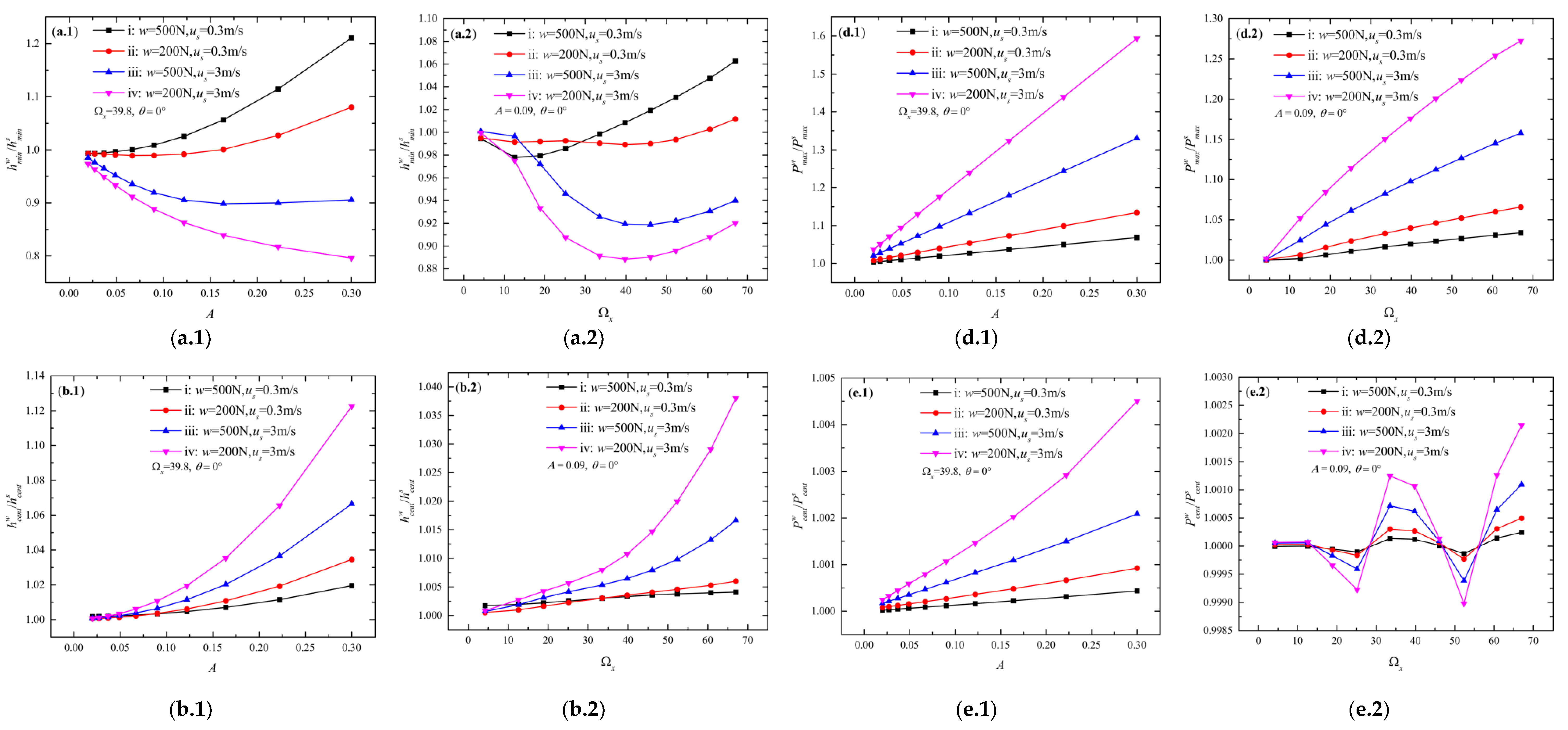
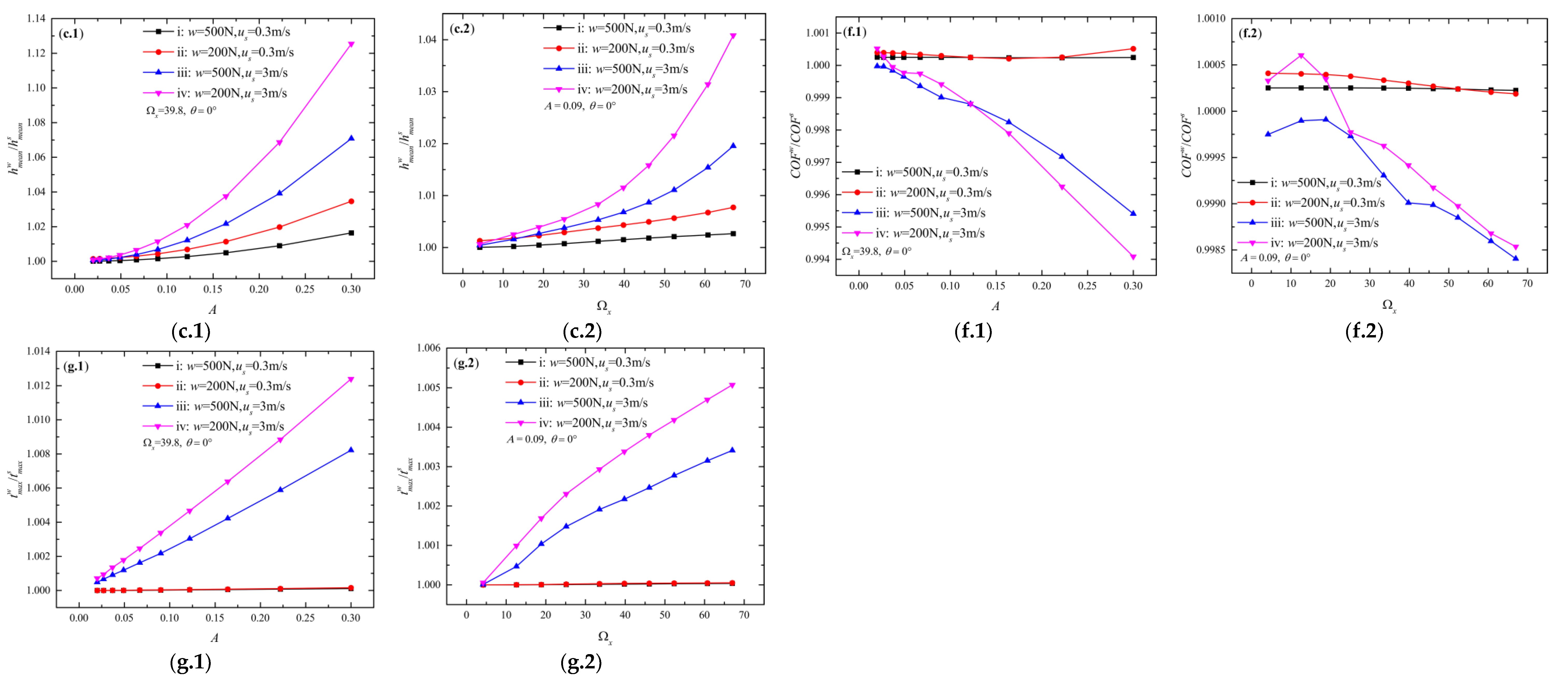
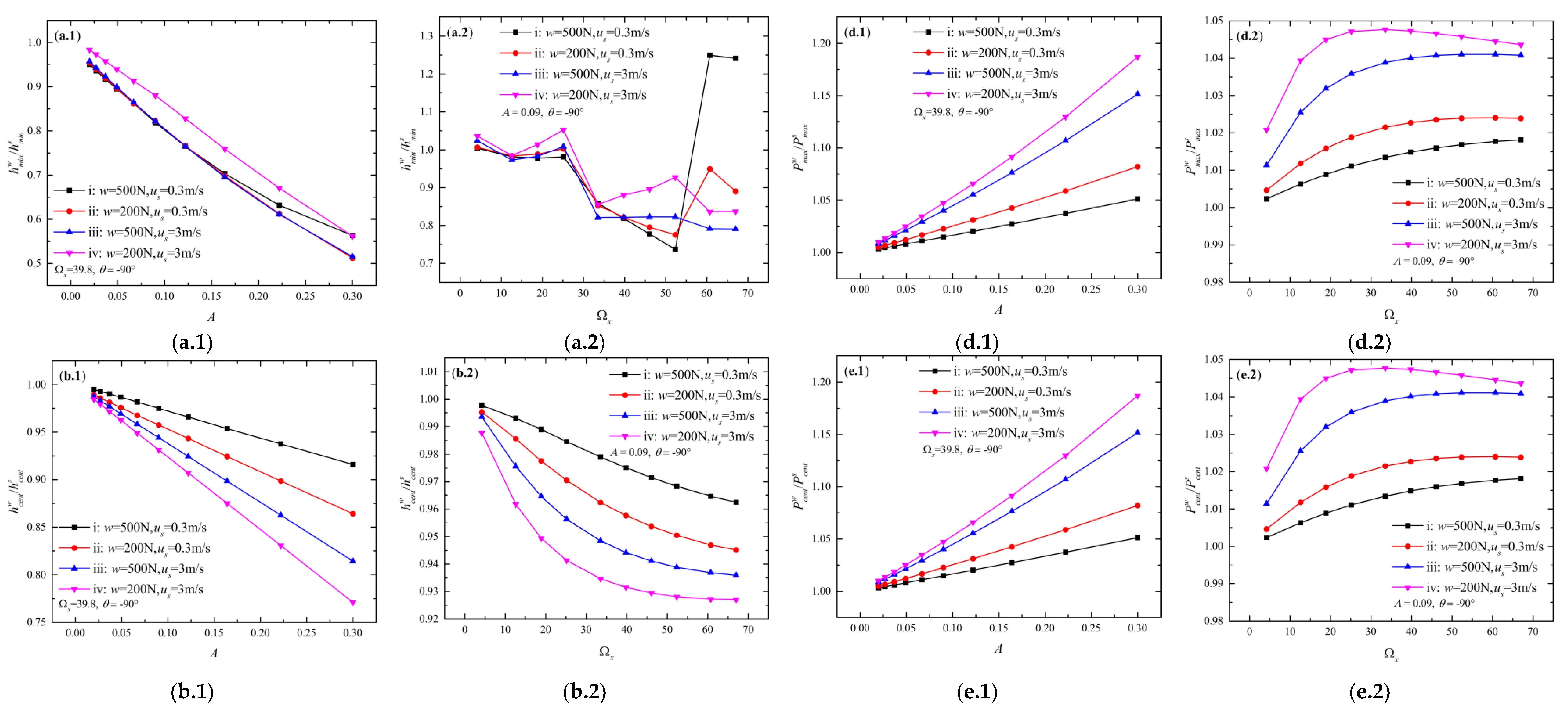
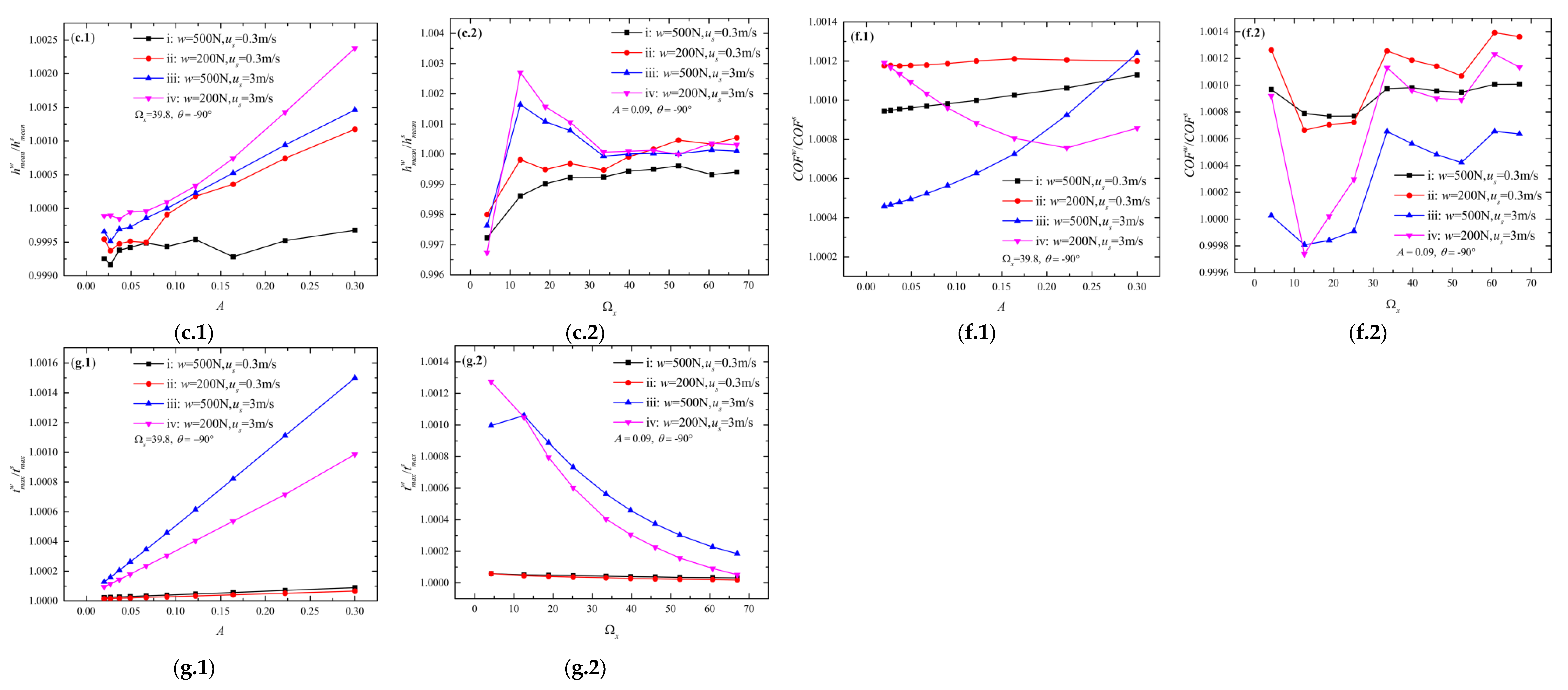
3.3. The Influences of the Load and Speed

According to Section 3.2, the three wave directions θ = 0°, −30°, and −60° result in similar contour maps, while longitudinal waviness leads to very different ones. The results regarding transverse and longitudinal waviness are discussed to represent and highlight the influences of the load and speed.
The two cross lines of each contour map, i.e., the lines with A = 0.09 or Ωx ≈ 39.8 (Nw = 19), were also extracted. Then, the extracted lines with the fixed wave direction (θ = 0° or θ = −90°), the same type of performance parameter, and the same constant A or Ωx were plotted in one graph. In each graph, the four curves representing the four combinations of loads (w = 200 N or 500 N) and speeds (us = 0.3 m/s or 3 m/s) show the impacts of the load and speed. The four combinations are indexed as i: (w = 500 N, us = 0.3 m/s), ii: (w = 200 N, us = 0.3 m/s), iii: (w = 500 N, us = 3 m/s), and iv: (w = 200 N, us = 3 m/s). As the working conditions change from i to iv, the corresponding smooth central (or minimum) film thickness increases (see Table 2). The thinner the film thickness is, the harsher the working conditions are. For one wave direction, there are fourteen such graphs. They are organized as sub-figures. Figure 8 shows the graphs for transverse waviness, where indices a to g represents the seven performance parameters, where ‘1’ and ‘2’ indicate the results of the fixed Ωx ≈ 39.8 and A = 0.09, respectively. Figure 9 shows the results for the longitudinal waviness in the same manner.
Figure 8a.1,a.2 shows that the h min w / h min s ratio is significantly affected by different working conditions. The h min w / h min s ratio decreases from greater to smaller than one as the working condition changes from i to iv for most of the A and Ωx values. Such results indicate that waviness can increase the minimum film thickness under harsh working conditions. As the working conditions become mild, the waviness gradually starts to decrease the minimum film thickness. Figure 8b,c shows that as the working condition changes in the same order (i to iv), the h c e n t w / h c e n t s and h m e a n w / h m e a n s ratios increase, and their values are greater than one. These results show that as the working conditions become milder, the increase in the central film thickness and mean film thickness with the waviness is more substantial.
Figure 8d,e illustrates the influences of the working conditions on the P max w / P max s and P c e n t w / P c e n t s ratios. It is clear that, regardless of how the ratios are affected by the A and Ωx values, changing the working condition from i to iv results in the increase in the P max w / P max s and P c e n t w / P c e n t s ratios. Figure 8f.1,f.2 shows that the effects of waviness on the COF are more significant at a higher speed (us = 3 m/s, conditions iii and iv). The same patterns are shown in Figure 8g.1,g.2, indicating that the maximum temperature rise is more closely related to the speed value. This phenomenon is expected, as the shear heat causes the temperature rise, being nearly proportional to the relative speed.
When the wave direction equals −90°, the influences of the working conditions have some unique features. Figure 9a.1,a.2 shows that the different working conditions (i to iv) have less impact on the h min w / h min s ratios compared with those shown in Figure 8a.1,a.2 (θ = 0°). In comparison, the h c e n t w / h c e n t s (Figure 9b) and h m e a n w / h m e a n s (Figure 9c) are more affected by the working conditions than the h min w / h min s ratio (Figure 9a). The h c e n t w / h c e n t s ratio decreases as A or Ωx increases (Figure 9b.1,b.2), in opposition to the trends shown in Figure 8b.1,b.2. Changing the working conditions from i to iv, the magnitude and speed of this decrease are enhanced. Such phenomena indicate that milder working conditions result in a thinner central film thickness when longitudinal waviness is used. The h m e a n w / h m e a n s ratio shown in Figure 9c.1 increases, with fluctuations, as the A increases. When the working condition becomes mild (i to iv), the magnitude and speed of this increase are enhanced. Figure 9c.2 illustrates that the h m e a n w / h m e a n s ratio rapidly increases and then decreases to a specific value as the Ωx increases. Such a trend differs from that shown in Figure 8c.2 (θ = 0°). As the working conditions change from i to iv, the magnitude and speed of the rapid increase phase are enhanced.
Figure 9d,e shows that the P max w / P max s and P c e n t w / P c e n t s ratios increase as the A or Ωx increases with the longitudinal waviness. When the working conditions change from i to iv, the magnitude and speed of this increase are enhanced. Figure 9f.1,f.2 shows that different working conditions affect the C O F w / C O F s ratios. However, it is difficult to define a specific law according to which the conditions affect the C O F w / C O F s ratio with longitudinal waviness. Figure 9g.1,g.2 shows the t max w / t max s ratios. Again, the results obtained at a higher speed (us = 3m/s, conditions iii and iv) are more sensitive to waviness.
It should be noted that working conditions iii and iv have different influences on the t max w / t max s ratio when comparing the results with θ = 0° and θ = −90°. When θ = 0°, condition iv results in a larger t max w / t max s ratio. However, condition iii results in a larger t max w / t max s ratio in most cases when θ = −90°.
In summary, the effects of the working conditions on the EHL performance with waviness are generally enhanced as the working conditions becomes mild. This work uses the non-dimensional amplitude and frequency of the waviness. The amplitude and frequency values are non-dimensionalized by the characteristic parameters of an EHL problem (Equations (6)–(8)). The same non-dimensional waviness indicates that the waviness incorporated is the same in terms of the scale compared with the EHL system. However, the same non-dimensional waviness leads to different results for different working conditions. These results reflect the nonlinear nature of the EHL system. One has to analyze the effects of waviness on the EHL performance on a case-by-case basis.
Additionally, there are two points to address. The minimum film thickness can be increased, to a certain extent, by non-longitudinal waviness when the working condition is harsh. This phenomenon should occur because the increase in the EHL contact caused by the waviness exceeds the minimum film thickness reduction caused by the wavy geometry. The COF and maximum temperature rise are more sensitive to the change in the speed than the change in the load. The reason for this should be that the friction force and the temperature rise are closely related to the shear stresses, which are strongly affected by the relative speed.

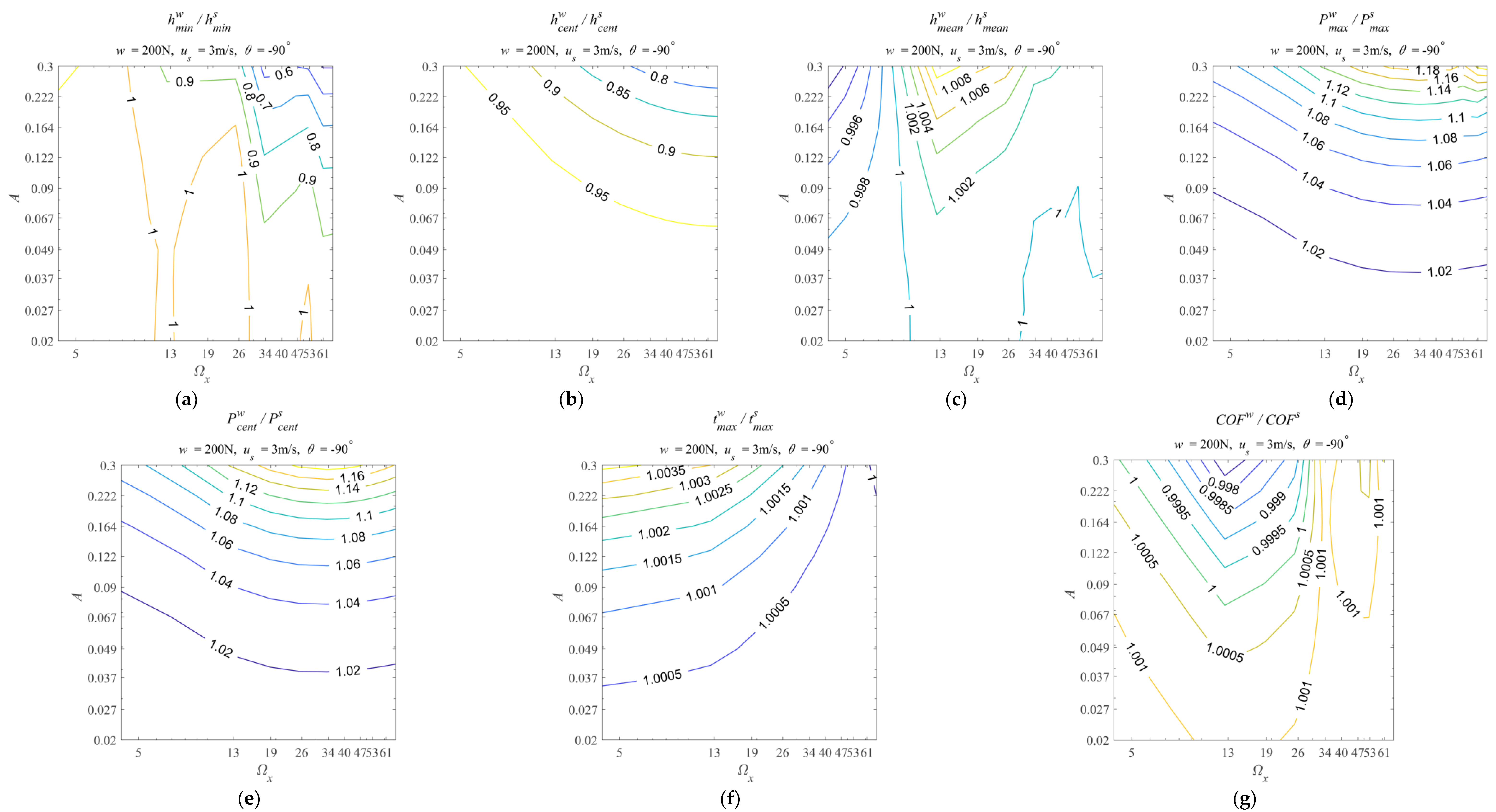
3.4. Further Remarks on the Contour Maps

The seven performance parameters are not independent, because they characterize the same EHL system in different aspects. According to the results outlined above, generally, incorporating waviness decreases the minimum film thickness but increases the central and mean film thickness. At the same time, the maximum pressure increases. The COF can be decreased, but the maximum temperature rise is increased simultaneously. If one wishes to utilize waviness as a beneficial factor in an EHL system, one should balance its influences on the different performance parameters. The simulated data and corresponding contour maps can be references for this purpose.
The other important point regarding the contour maps is that they provide a possible way to identify the relevant roughness scales when simulating point EHL problems. The contour maps are plotted on the double-logarithmic Ωx-A coordinate system. A specific contour line describes the amplitude–frequency relationship (Ωx, A), according to which the response of the EHL system to the waviness on different scales is fixed to specific levels. For rough surfaces, the power spectral density (PSD) characterizes the multiscale properties of rough surfaces [13]. The PSD is also plotted on the double-logarithmic coordinate system.
Figure 10 shows the PSD of a measured lapping surface on the double-logarithmic coordinate system. The abscissa is the angular frequency, and the ordinate is the power spectrum magnitude corresponding to different frequencies. It should be noted that the power spectrum magnitude is related to the surface root mean square (RMS) roughness, or in other words, the amplitude of the roughness. Hence, the PSD describes the frequency–amplitude relationship of rough surfaces.
Therefore, if one transforms the PSD into the contour map coordinates and plots them in the exact figure, the relative position of the contour lines and PSD can indicate the magnitude of the roughness influences on the EHL performance within different frequency ranges. Furthermore, if the contour line plotted represents the criterion that one uses to determine whether or not the roughness significantly affects the EHL performance, the figure can help one to identify the roughness scales relevant to the EHL simulation. This idea will be investigated and developed in our future work.

4. Conclusions

This paper discussed the influences of multiscale waviness on the full-film EHL performance. Multiscale waviness was generated with different amplitudes, frequencies, and directions. We found that the amplitude and frequency are related to the central film thickness and the Hertzian contact radius of the corresponding smooth EHL problems, respectively. Then, multiscale waviness was input to a transient TEHL model under different working conditions. Seven performance parameters of an EHL system were extracted from the simulation results. The ratios of these parameters with and without waviness were discussed in detail. The main conclusions are as follows:
  • The transverse and oblique waviness lead to similar results. The minimum film thickness decreases in most cases and can reach a minimum value with a specific combination of amplitude and frequency. Increasing the amplitude and frequency usually increases the central and mean film thickness and maximum pressure but slightly affects the central pressure. Moreover, increasing the amplitude and frequency results in a smaller COF with a higher maximum temperature rise.
  • With the waviness shifting toward the longitudinal direction, this usually decreases the minimum, central, and mean film thickness and COF. At the same time, the maximum pressure, central pressure, and maximum temperature rise are only slightly affected.
  • The longitudinal waviness leads to different results compared with the other wave directions. It increases the minimum film thickness in some cases, decreases the central film thickness, and slightly affects the mean film thickness, COF, and maximum temperature rise. Moreover, it decreases the maximum pressure but increases the central pressure.
  • The effects of the working conditions on the EHL performance under the condition of waviness are generally enhanced as the working conditions become mild. The minimum film thickness can be increased by non-longitudinal waviness, to a certain extent, when the working condition is harsh. The COF and maximum temperature rise are more sensitive to the change in the speed than the change in the load.
  • One who wishes to utilize waviness as a beneficial factor in an EHL system should balance its influences on the different performance parameters. The simulated data and corresponding contour maps can be used as a reference for this purpose (see Supplementary Material S2).
Furthermore, combining the contour maps and PSD of the roughness could provide a way of identifying the relevant roughness scales when simulating point EHL problems. This idea will be investigated and developed in our future work. Moreover, the fixed SRR (−0.2) limits the influences of the waviness on the COF and maximum temperature rise. Studies using various SRR values will be conducted in our future work as well.

Supplementary Materials

The following supporting information can be downloaded at: https://www.mdpi.com/article/10.3390/lubricants10120368/s1, ‘Supplemental Material S1.pdf’, ‘Supplemental Material S2.zip’, including the folder: ‘ContourMaps’ and ‘Results_simulated.xlsx’.

Author Contributions

Conceptualization, Y.W.; methodology, Y.W.; software, Y.W.; validation, Y.W.; formal analysis, Y.W.; data curation, Y.W. and C.L.; writing—original draft preparation, Y.W.; writing—review and editing, Y.W., C.L, J.D. and A.M.; visualization, Y.W. and C.L.; supervision, J.D. and A.M.; project administration, A.M.; funding acquisition, A.M. and Y.W. All authors have read and agreed to the published version of the manuscript.

Funding

This research was funded by the Engineering and Physical Sciences Research Council, grant number EP/S030476/1, and Harbin Institute of Technology, Shenzhen, grant number 20220068”.

Data Availability Statement

The data that support the findings of this study are available from the corresponding author, Y.W., upon reasonable request.

Acknowledgments

Many thanks to Erik Hansen, Institute of Fluid Mechanics, Karlsruhe Institute of Technology (KIT), for the discussions and comments on the current work. This work was undertaken at ARC3, part of the High-Performance Computing facilities at the University of Leeds, UK.

Conflicts of Interest

The authors declare no conflict of interest. The funders had no role in the design of the study; in the collection, analyses, or interpretation of data; in the writing of the manuscript; or in the decision to publish the results.

Nomenclature

adimensional amplitude of the waviness, m
Anon-dimensional amplitude of waviness
bradius of the Hertzian contact zone, m
M, Nnumber of grids in the X and Y directions, respectively
C O F w / C O F s ratio of the COF with and without waviness
h min w / h min s ratio of the minimum film thickness with and without waviness
h c e n t w / h c e n t s ratio of the central film thickness with and without waviness
h m e a n w / h m e a n s ratio of the mean film thickness with and without waviness
NTtime step for the termination of the simulation
Nwnumber of waves in the solution domain
P max w / P max s ratio of the maximum pressure with and without waviness
P c e n t w / P c e n t s ratio of the central pressure with and without waviness
rθwaviness in direction θ, m
t max w / t max s ratio of the maximum temperature rise with and without waviness
non-dimensional time in the simulation
Δ t ¯ non-dimensional time interval of the simulation
u1velocity of the smooth surface, m/s
u2velocity of the waviness, m/s
ussum of u1 and u2, m/s
Unon-dimensional speed
wload, N
Xs, Xenon-dimensional start and end coordinates of the solution domain in the X direction
Ys, Yenon-dimensional start and end coordinates of the solution domain in the Y direction
X s   ,   Y s   non-dimensional start of waviness at t ¯ = 0 with the wave direction θ
αviscosity–pressure coefficient in the Barus viscosity law, Pa−1
θwave direction, degree
Λxnon-dimensional wavelength of the waviness
Ωxnon-dimensional frequency of the waviness

References

  1. Vakis, A.; Yastrebov, V.; Scheibert, J.; Nicola, L.; Dini, D.; Minfray, C.; Almqvist, A.; Paggi, M.; Lee, S.; Limbert, G.; et al. Modeling and simulation in tribology across scales: An overview. Tribol. Int. 2018, 125, 169–199. [Google Scholar] [CrossRef]
  2. Pei, X.; Pu, W.; Zhang, Y.; Huang, L. Surface topography and friction coefficient evolution during sliding wear in a mixed lubricated rolling-sliding contact. Tribol. Int. 2019, 137, 303–312. [Google Scholar] [CrossRef]
  3. Wang, X.; Xu, Y.; Jackson, R.L. Theoretical and Finite Element Analysis of Static Friction Between Multi-Scale Rough Surfaces. Tribol. Lett. 2018, 66, 146. [Google Scholar] [CrossRef]
  4. Li, Q.; Pohrt, R.; Popov, V.L. Adhesive Strength of Contacts of Rough Spheres. Front. Mech. Eng. 2019, 5, 7. [Google Scholar] [CrossRef] [Green Version]
  5. Violano, G.; Afferrante, L. Contact of rough surfaces: Modeling adhesion in advanced multiasperity models. Proc. Inst. Mech. Eng. Part J J. Eng. Tribol. 2019, 233, 1585–1593. [Google Scholar] [CrossRef]
  6. Brunetière, N.; Francisco, A. Lubrication Mechanisms Between Parallel Rough Surfaces. Tribol. Lett. 2019, 67, 116. [Google Scholar] [CrossRef] [Green Version]
  7. Zhang, X.; Xu, Y.; Jackson, R.L. A mixed lubrication analysis of a thrust bearing with fractal rough surfaces. Proc. Inst. Mech. Eng. Part J J. Eng. Tribol. 2019, 234, 608–621. [Google Scholar] [CrossRef]
  8. Pérez-Ràfols, F.; Almqvist, A. On the stiffness of surfaces with non-Gaussian height distribution. Sci. Rep. 2021, 11, 1863. [Google Scholar] [CrossRef]
  9. Belhadjamor, M.; Belghith, S.; Mezlini, S.; El Mansori, M. Numerical study of normal contact stiffness: Non-Gaussian roughness and elastic–plastic behavior. Proc. Inst. Mech. Eng. Part J J. Eng. Tribol. 2020, 234, 1368–1380. [Google Scholar] [CrossRef]
  10. Wang, Y.; Dorgham, A.; Liu, Y.; Wang, C.; Ghanbarzadeh, A.; Wilson, M.C.T.; Neville, A.; Azam, A. Towards optimum additive performance: A numerical study to understand the influence of roughness parameters on the zinc dialkyldithiophosphates tribofilm growth. Lubr. Sci. 2021, 33, 1–14. [Google Scholar] [CrossRef]
  11. Archard, J.F. Elastic deformation and the laws of friction. Proc. R. Soc. Lond. Ser. A Math. Phys. Sci. 1957, 243, 190–205. [Google Scholar] [CrossRef]
  12. Whitehouse, D.J.; Archard, J.F. The properties of random surfaces of significance in their contact. Proc. R. Soc. Lond. Ser. A Math. Phys. Sci. 1970, 316, 97–121. [Google Scholar] [CrossRef] [Green Version]
  13. Sayles, R.S.; Thomas, T.R. Surface topography as a nonstationary random process. Nature 1978, 271, 431–434. [Google Scholar] [CrossRef]
  14. Nayak, P.R. Random Process Model of Rough Surfaces. J. Lubr. Technol. 1971, 93, 398–407. [Google Scholar] [CrossRef]
  15. Longuet-Higgins, M.S. Statistical properties of an isotropic random surface. Philos. Trans. R. Soc. Lond. Ser. A Math. Phys. Sci. 1957, 250, 157–174. [Google Scholar] [CrossRef]
  16. Mandelbrot, B.B. The Fractal Geometry of Nature; Times Books: New York, NY, USA, 1983; Volume 173. [Google Scholar]
  17. Majumdar, A.; Tien, C.L. Fractal characterization and simulation of rough surfaces. Wear 1990, 136, 313–327. [Google Scholar] [CrossRef]
  18. Majumdar, A.; Bhushan, B. Fractal Model of Elastic-Plastic Contact between Rough Surfaces. J. Tribol. 1991, 113, 1–11. [Google Scholar] [CrossRef]
  19. Bhushan, B.; Majumdar, A. Elastic-plastic contact model for bifractal surfaces. Wear 1992, 153, 53–64. [Google Scholar] [CrossRef]
  20. Persson, B.N.J. Theory of rubber friction and contact mechanics. J. Chem. Phys. 2001, 115, 3840–3861. [Google Scholar] [CrossRef] [Green Version]
  21. Müser, M.H.; Dapp, W.B.; Bugnicourt, R.; Sainsot, P.; Lesaffre, N.; Lubrecht, T.A.; Persson, B.N.J.; Harris, K.; Bennett, A.; Schulze, K.; et al. Meeting the Contact-Mechanics Challenge. Tribol. Lett. 2017, 65, 118. [Google Scholar] [CrossRef]
  22. Persson, B.N.J.; Albohr, O.; Tartaglino, U.; Volokitin, A.; Tosatti, E. On the nature of surface roughness with application to contact mechanics, sealing, rubber friction and adhesion. J. Phys. Condens. Matter 2004, 17, R1. [Google Scholar] [CrossRef] [PubMed] [Green Version]
  23. Majumdar, A.; Tien, C.L. Fractal network model for contact conductance. J. Heat Transf. 1991, 113, 516–525. [Google Scholar] [CrossRef]
  24. Barber, J.R. Bounds on the electrical resistance between contacting elastic rough bodies. Proc. R. Soc. A Math. Phys. Eng. Sci. 2003, 459, 53–66. [Google Scholar] [CrossRef] [Green Version]
  25. Patir, N.; Cheng, H.S. An average flow model for determining effects of three-dimensional roughness on partial hydrodynamic lubrication. J. Lubr. Technol. 1979, 100, 12–17. [Google Scholar] [CrossRef]
  26. Patir, N.; Cheng, H.S. Application of average flow model to lubrication between rough sliding surfaces. J. Lubr. Technol. 1979, 101, 220–230. [Google Scholar] [CrossRef]
  27. Patir, N. Effect of surface roughness orientation on the central film thickness in EHD Contacts. Proc. Inst. Mech. Engl. Part I 1979, 185, 15–21. [Google Scholar]
  28. Almqvist, A.; Fabricius, J.; Spencer, A.; Wall, P. Similarities and Differences Between the Flow Factor Method by Patir and Cheng and Homogenization. J. Tribol. 2011, 133, 031702. [Google Scholar] [CrossRef]
  29. Almqvist, A.; Lukkassen, D.; Meidell, A.; Wall, P. New concepts of homogenization applied in rough surface hydrodynamic lubrication. Int. J. Eng. Sci. 2007, 45, 139–154. [Google Scholar] [CrossRef] [Green Version]
  30. Bayada, G.; Martin, S.; Vázquez, C. Two-scale homogenization of a hydrodynamic Elrod-Adams model. Asymptot. Anal. 2005, 44, 75–110. [Google Scholar]
  31. Almqvist, A.; Dasht, J. The homogenization process of the Reynolds equation describing compressible liquid flow. Tribol. Int. 2006, 39, 994–1002. [Google Scholar] [CrossRef]
  32. Sahlin, F.; Larsson, R.; Almqvist, A.; Lugt, P.; Marklund, P. A mixed lubrication model incorporating measured surface topography. Part 1: Theory of flow factors. Proc. Inst. Mech. Eng. Part J J. Eng. Tribol. 2009, 224, 335–351. [Google Scholar] [CrossRef] [Green Version]
  33. Zhao, Y.; Liu, H. Analysis of the effect of surface topography on lubrication using heterogeneous multiscale method. Tribol. Int. 2021, 158, 106922. [Google Scholar] [CrossRef]
  34. Pei, S.; Xu, H.; Shi, F. A deterministic multiscale computation method for rough surface lubrication. Tribol. Int. 2016, 94, 502–508. [Google Scholar] [CrossRef]
  35. Nyemeck, A.P.; Brunetière, N.; Tournerie, B. A Mixed Thermoelastohydrodynamic Lubrication Analysis of Mechanical Face Seals by a Multiscale Approach. Tribol. Trans. 2015, 58, 836–848. [Google Scholar] [CrossRef]
  36. Zhu, D.; Ai, X. Point contact EHL based on optically measured three-dimensional rough surfaces. J. Tribol. 1997, 119, 375–384. [Google Scholar] [CrossRef]
  37. Minet, C.; Brunetière, N.; Tournerie, B. Mixed Lubrication Modelling in Mechanical Face Seals. In Proceedings of the STLE/ASME International Joint Tribology Conference 2008, Miami, FL, USA, 20–22 October 2008; pp. 477–479. [Google Scholar]
  38. Ren, N.; Zhu, D.; Chen, W.W.; Liu, Y.; Wang, Q.J. A Three-Dimensional Deterministic Model for Rough Surface Line-Contact EHL Problems. J. Tribol. 2008, 131, 011501. [Google Scholar] [CrossRef]
  39. Demirci, I.; Mezghani, S.; Yousfi, M.; El Mansori, M. Multiscale Analysis of the Roughness Effect on Lubricated Rough Contact. J. Tribol. 2013, 136, 011501. [Google Scholar] [CrossRef] [Green Version]
  40. Lorentz, B.; Albers, A. A numerical model for mixed lubrication taking into account surface topography, tangential adhesion effects and plastic deformations. Tribol. Int. 2013, 59, 259–266. [Google Scholar] [CrossRef]
  41. Zhu, D.; Wang, Q.J. Effect of Roughness Orientation on the Elastohydrodynamic Lubrication Film Thickness. J. Tribol. 2013, 135, 031501. [Google Scholar] [CrossRef]
  42. Zhu, D.; Wang, J.; Wang, Q.J. On the Stribeck Curves for Lubricated Counterformal Contacts of Rough Surfaces. J. Tribol. 2015, 137, 021501. [Google Scholar] [CrossRef]
  43. Li, L.; Yang, J. Surface roughness effects on point contact elastohydrodynamic lubrication in linear rolling guide with fractal surface topographies. Ind. Lubr. Tribol. 2018, 70, 589–598. [Google Scholar] [CrossRef]
  44. Pei, J.; Han, X.; Tao, Y.; Feng, S. Mixed elastohydrodynamic lubrication analysis of line contact with Non-Gaussian surface roughness. Tribol. Int. 2020, 151, 106449. [Google Scholar] [CrossRef]
  45. Venner, C.H.; Lubrecht, A.A. An Engineering Tool for the Quantitative Prediction of General Roughness Deformation in EHL Contacts Based on Harmonic Waviness Attenuation. Proc. Inst. Mech. Eng. Part J J. Eng. Tribol. 2005, 219, 303–312. [Google Scholar] [CrossRef]
  46. Bair, S.; Winer, W.O. The High Pressure High Shear Stress Rheology of Liquid Lubricants. J. Tribol. 1992, 114, 1–9. [Google Scholar] [CrossRef]
  47. Wang, Y.; Dorgham, A.; Liu, Y.; Wang, C.; Wilson, M.C.T.; Neville, A.; Azam, A. An Assessment of Quantitative Predictions of Deterministic Mixed Lubrication Solvers. J. Tribol. 2020, 143, 011601. [Google Scholar] [CrossRef]
  48. He, T.; Zhu, D.; Wang, J.; Wang, Q.J. Experimental and Numerical Investigations of the Stribeck Curves for Lubricated Counterformal Contacts. J. Tribol. 2016, 139, 021505. [Google Scholar] [CrossRef]
  49. Pu, W.; Wang, J.; Zhu, D. Progressive Mesh Densification Method for Numerical Solution of Mixed Elastohydrodynamic Lubrication. J. Tribol. 2015, 138, 021502. [Google Scholar] [CrossRef]
  50. Wang, W.-Z.; Hu, Y.-Z.; Liu, Y.-C.; Zhu, D. Solution agreement between dry contacts and lubrication system at ultra-low speed. Proc. Inst. Mech. Eng. Part J J. Eng. Tribol. 2010, 224, 1049–1060. [Google Scholar] [CrossRef]
  51. Venner, C.H.; Lubrecht, A.A. Numerical Analysis of the Influence of Waviness on the Film Thickness of a Circular EHL Contact. J. Tribol. 1996, 118, 153–161. [Google Scholar] [CrossRef]
  52. Ehret, P.; Dowson, D.; Taylor, C. Waviness Orientation in EHL Point Contact. In The Third Body Concept Interpretation of Tribological Phenomena; Dowson, D., Taylor, C.M., Childs, T.H.C., Dalmaz, G., Berthier, Y., Flamand, L., Georges, J.-M., Lubrecht, A.A., Eds.; Tribology Series; Elsevier: Amsterdam, The Netherlands, 1996; Volume 31, pp. 235–244. [Google Scholar] [CrossRef]
  53. Reddyhoff, T.; Schmidt, A.; Spikes, H. Thermal Conductivity and Flash Temperature. Tribol. Lett. 2019, 67, 22. [Google Scholar] [CrossRef] [Green Version]
  54. Liu, H.; Zhang, B.; Bader, N.; Poll, G.; Venner, C. Influences of solid and lubricant thermal conductivity on traction in an EHL circular contact. Tribol. Int. 2020, 146, 106059. [Google Scholar] [CrossRef]
  55. Habchi, W.; Bair, S. The role of the thermal conductivity of steel in quantitative elastohydrodynamic friction. Tribol. Int. 2020, 142, 105970. [Google Scholar] [CrossRef]
  56. Pu, W.; Zhu, D.; Wang, J. A Starved Mixed Elastohydrodynamic Lubrication Model for the Prediction of Lubrication Performance, Friction and Flash Temperature with Arbitrary Entrainment Angle. J. Tribol. 2017, 140, 031501. [Google Scholar] [CrossRef]
Figure 1. Solution domain of the EHL problem.
Lubricants 10 00368 g001
Figure 2. Wavy surface with an arbitrary direction angle.
Lubricants 10 00368 g002
Figure 3. Contour maps related to the film thickness parameters, w = 200 N, us = 0.3 m/s, θ = 0°, (a) h min w / h min s , (b) h c e n t w / h c e n t s , and (c) h m e a n w / h m e a n s .
Lubricants 10 00368 g003aLubricants 10 00368 g003b
Figure 4. Contour maps related to the pressure parameters, w = 200 N, us = 0.3 m/s, θ = 0°, (a) P max w / P max s , and (b) P c e n t w / P c e n t s .
Lubricants 10 00368 g004
Figure 5. The (a) C O F w / C O F s and (b) t max w / t max s contour maps, w = 200 N, us = 0.3 m/s, θ = 0°.
Lubricants 10 00368 g005
Figure 6. Performance parameters with w = 200 N, us = 3 m/s, θ = 0°, −30°, −60°, and −90°. Here, a to g are (a) h min w / h min s , (b) h c e n t w / h c e n t s , (c) h m e a n w / h m e a n s , (d) P max w / P max s , (e) P c e n t w / P c e n t s , (f) C O F w / C O F s , (g) t max w / t max s . ‘1’ indicates the results of fixed Ωx ≈ 39.8, and ‘2’ indicates the results of fixed A = 0.09.
Lubricants 10 00368 g006aLubricants 10 00368 g006b
Figure 7. Contour maps of the seven performance parameters with w = 200 N, us = 3 m/s, and θ = −90°, (a) h min w / h min s , (b) h c e n t w / h c e n t s , (c) h m e a n w / h m e a n s , (d) P max w / P max s , (e) P c e n t w / P c e n t s , (f) C O F w / C O F s , and (g) t max w / t max s .
Lubricants 10 00368 g007
Figure 8. Performance parameters with θ = 0°, w = 200 N, 500 N, us = 0.3 m/s, 3 m/s. Indices a to g are (a,b) h c e n t w / h c e n t s , (c) h m e a n w / h m e a n s , (df) C O F w / C O F s , and (g) t max w / t max s . ‘1’ indicates the results of fixed Ωx ≈ 39.8, and ‘2’ indicates the results of fixed A = 0.09.
Lubricants 10 00368 g008aLubricants 10 00368 g008b
Figure 9. Performance parameters with θ = −90°, w = 200 N, 500 N, us = 0.3 m/s, 3 m/s. Here, a to g are (a) h min w / h min s , (b) h c e n t w / h c e n t s , (c) h m e a n w / h m e a n s , (d) P max w / P max s , (e) P c e n t w / P c e n t s , (f) C O F w / C O F s , and (g) t max w / t max s . ‘1’ indicates the results of fixed Ωx ≈ 39.8, and ‘2’ indicates the results of fixed A = 0.09.
Lubricants 10 00368 g009aLubricants 10 00368 g009b
Figure 10. PSD of a measured lapping surface.
Lubricants 10 00368 g010
Table 1. Basic parameters of the EHL simulation.
ParameterDisk (Body 1)Ball (Body 2)Fluid
Young’s modulus, (GPa)206206
Poisson’s ratio0.30.3
Density, (g/cm3)7.8657.8650.8433
Thermal conductivity, (W/(m∙K))46460.145
Specific heat, (N∙m/(g∙K))0.460.462
Thermal expansivity (K−1)0.00064
Viscosity at 40 °C, (Pa∙s)0.0279
Temperature–viscosity coefficient, (K−1)0.029
Pressure–viscosity coefficient, (GPa−1)22.224
Ball radius, (m)9.525 × 10⁻³
Slide-to-roll ratio, SRR−0.2
Table 2. Central and minimum film thickness of the four working conditions without waviness.
Load, w (N)200500
Speed, us (m/s)0.330.33
Central   film   thickness ,   h c e n t s (μm)0.06770.32780.06280.3152
Minimum   film   thickness ,   h min s (μm)0.01810.14650.01040.1141
Average film thickness, h m e a n s (μm)0.06170.30040.05710.2867
Central pressure, P c e n t s (GPa)1.11281.12271.50811.5167
Maximum pressure, P max s (GPa)1.11281.12281.50811.5168
Coefficient of friction, C O F s 0.08190.07300.08820.0759
Maximum temperature rise, t max s (K)317.9658332.5601321.5860343.0376
Table 3. The range of performance parameter ratios obtained with w = 200 N, us = 3 m/s, and θ = 0°.
ParameterMinMax
Minimum   film   thickness   ratio ,   h min w / h min s 0.7721.000
Central   film   thickness   ratio ,   h c e n t w / h c e n t s 1.0001.451
Average   film   thickness   ratio ,   h m e a n w / h m e a n s 1.0001.423
Maximum   pressure   ratio ,   P max w / P max s 1.0002.042
Central   pressure   ratio ,   P c e n t w / P c e n t s 0.9981.016
COF   ratio ,   C O F w / C O F s 0.9831.001
Maximum   temperature   rise   ratio ,   t max w / t max s 1.0001.030
Publisher’s Note: MDPI stays neutral with regard to jurisdictional claims in published maps and institutional affiliations.

