Abstract
This paper presents a detailed three-dimensional (3D) thermo-elastic-hydrodynamic (TEHD) multi-physics model of the bump-type gas foil thrust bearing based on computational fluid dynamics (CFD). In this model, the moving mesh technology is applied in the fluid flow domain, and the new boundary condition of fully developed flow is applied at the inlet and outlet boundaries, which is consistent with the continuous property of fluid flow and has better convergence performance in CFD. The groove between pads is set as the symmetry boundary. The contact pairs with Coulomb friction and contact/separation behaviors are considered in the structure deformation and heat transfer. The simulation results indicated that the boundary pressure has a significant influence on the foil deformation. It also revealed the heat flux transfer path and temperature distribution in the gas foil thrust-bearing (GFTB) system.
1. Introduction
GFTB is an environmentally friendly hydrodynamic bearing that withstands axial load, which is widely used in high-speed turbomachinery due to its advantages of higher reliability, lower operating costs, and soft failure, etc. [1]. As the requirements of rotational speed increase and the operating environment became complex, the traditional calculation methods with assumptions of constant temperature cannot accurately predict the bearing performance [2].
Theoretical and experimental research considering the influence of temperature has been conducted. Scholars have established different forms of temperature field calculation models of gas foil bearings. Salehi et al. [3] simplified the energy equation by using the Couette approximation method to handle the relationship between air viscosity and temperature, but ignored the influence of the axial pressure gradient with only circumferential temperature distribution being calculated. Peng et al. [4] simplified the foil structure as a spring model to couple Reynolds equations with heat transfer equations. They considered the forced convection outside the top foil, but ignored the heat transfer to the rotor and bearing sleeve. Paulsen et al. [5] compared the differences in the results of dynamic characteristics based on isothermal and thermal models of three different types of journal foil bearing. However, the axial heat flux in the shaft was not considered, and the calculated temperature was a bit too high. Lee et al. [6] presented the heat transfer models of top foil, bump foil, cooling channel, and thrust plate in detail under the symmetric arrangement of two GFTBs and considered the effect of temperature on gas viscosity in Reynolds’ equation. However, the bump foil was simplified as a lumped thermal mass model. Hu et al. [7] established a nonlinear bump stiffness model considering the friction force and obtained the performance of GFTBs by coupling the foil deformation equation with Reynolds and energy equations. Those models mentioned above calculated the flow field by solving the two-dimensional (2D) Reynolds equation and simplified the foil structure and heat transfer to some extent.
Detailed TEHD models take more factors into account, including the rotor thermal expansion, cooling flow, turbulence flow, etc. Gad et al. [8] modeled the fluid flow with a 2D compressible Reynolds equation and obtained the temperature distribution of GFTBs by the Couette approximation method. They considered the cooling flow and backing flow in their model. Feng [9] established the 3D THD model that considered heat convection into cooling air, thermal expansion, and material property variations due to temperature rise. Sim and Kim [10] presented a 3D THD model by taking the heat transfer of the rotor and bearing sleeve into account instead of assuming they are thermal boundary conditions. Rieken [11] established a detailed TEHD model that considered foil deformations with the shell theory and also introduced the bearing dry friction between foils. The thermal model includes the base plate, rotor disk, heat fluxes into rotor and periphery of the bearing, and cooling flow on the backside of the rotor disk. Lehn et al. [12] calculated the thermal resistance of bump foil/top foil and bump foil/backing plate. They considered the heat flux of the small gap between the thrust disk and the housing, the thermal expansion of the thrust disk, and the self-induced cooling flow on the thrust disk back. Xu et al. [13] established a 3D thermal-hydrodynamic analyzed of GFTBs for both CO2 and R245fa and considered real gas effect and flow turbulence inside the film. However, the aforementioned models did not consider a complex boundary condition.
To improve the accuracy of the fluid model in foil bearings, computational fluid dynamics (CFD) was applied in the TEHD model. Aksoy et al. [14] used the finite element code provided by commercial software to solve the Reynolds equation and structural deformation simultaneously, which are further coupled with the self-developed FDM code to solve the energy equation. Their model considered the physical contacts between bearing assembly components. Xu et al. [15] established a CFD model to predict the pressure distribution and capacity of GFTB and improved the simulation by modifying air parameters obtained from experiments. They also considered the ambient temperature within 200 °C. Fu [16,17] created a 3D CFD model to simulate the static properties of GFTBs by using a goal-driven optimization technique to improve the load capacity and reduce the maximum temperature. However, the structural deformation results were not presented. Qin et al. [18,19,20] developed a 3D THED model by using the CFD code Eilmer, considering the detailed structure model, complex fluid flow, CO2 medium, turbulence, and wall function, etc., which helped to predict the bearing performance more accurately. Kim et al. [21] considered the leading-edge groove region as the inlet thermal boundary conditions in the CFD model and developed the THD model by extending the solution domain to surrounding structures. They evaluated the dynamic performance at an elevated temperature and also found that the softening effect of the bump foil results in a decrease of both stiffness and damping coefficients. Ravikovich et al. [22] established a CFD model for the fluid domain and incorporated the analytical expressions for the deformation of compliant elements into the CFD model through a moving mesh technique. Thus, the structural model was extremely simplified. Supreeth et al. [23] designed and fabricated a GFTB to optimize the foil stiffness in terms of foil thickness with the experiments at various configurations and also carried out the related CFD simulation, but the mesh of the CFD model they established is quite rough. Yu et al. [24] built a CFD model to simulate the dynamic characteristics of the GFTB, whereas the bump foils were simplified as Hooke springs attached to top foil with a small amount of deformation. In general, most of the CFD models have not taken into account the detailed foil structure and have considered more detailed boundary conditions.
Compared with the above references, the TEHD model established in this paper considered the fully developed flow boundary conditions, the fluid domain contents, and the groove parts, and the structure domain also considers more actual detached contacts. The paper is organized as follows. First, all the governing equations and principles involved in each physical field were introduced. Secondly, the model reliability was verified by comparing it with the literature results and the numerical simulations. Finally, the thermal transfer, structural deformation, and hydrodynamic performance of gas foil thrust bearings under different conditions were analyzed.
2. Methodology
In this study, the three-dimensional TEHD computational model is established by using COMSOL software, which consists of three coupled physical fields: fluid flow, structural deformation, and heat transfer. In this section, the main problems involved in each single physical field and coupled physical fields are described, respectively.
2.1. Geometrical Model and Computational Domain of GFTB
The detailed structure of bump-type thrust bearing with six pads is shown in Figure 1, which mainly consists of a smooth surface top foil with a slight slope segment and a plane segment to provide gas lubricating conditions. The bump foil, shaped of corrugated and flat parts that are alternately connected, is located under the plane section of top foil to provide elastic support. The spacer shim is used to adjust the slope height δh, and a backing plate is used to fix the three components above.
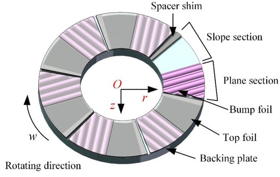
Figure 1.
Three-dimensional geometrical model of GFTB.
Due to the assumption of neglecting misalignment of thrust runner, the computational domains of the entire bearing structure and fluid including six integrated pads could be simplified to one considering the rotational symmetry boundary conditions of sectoral gas film. The investigation of thermal characteristics is also conducted based on the above simplified one-pad mode, which could greatly reduce the computational workload. The final model of the physics domains is presented in Figure 2.
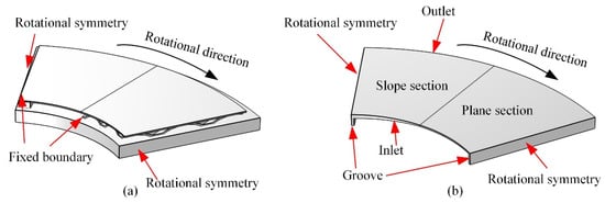
Figure 2.
Simplified domain. (a) Structure computational domain. (b) Fluid computational domain (the z-direction is stretched 10 times).
The pressure distribution and the comparison of load capacity for the entire CFD model and symmetry CFD model are illustrated in Figure 3. It is concluded that the pressure distribution is the same for those two models and the magnitude of load capacity is also relatively similar where the errors E0 are less than 1.6 × 10⁻⁴ in the situations of this model. E0 = (F2 – F1)/F1, where F1 (N) is the load capacity of entire model, and F2 (N) is the load capacity of simplified symmetry model. Thus, the simplified symmetry model can be applied to subsequent analysis.
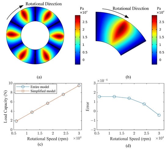
Figure 3.
The verification of the entire CFD model and symmetry CFD model. (a) Pressure distribution of entire model. (b) Pressure distribution of symmetry model. (c) Comparison of load capacity. (d) Errors of load capacity between the two models.
2.2. Modeling of Fluid Flow
In the fluid component of this model, the gas film is assumed to be compressible fluid flow, the full Naiver–Stokes equations are solved by CFD software utilizing a finite element approach, and relevant fluid-governing equations are presented as follows. The continuity equation is formulated as
where ρ is the density of fluid (kg/m3) and u is the velocity vector (m/s). The momentum equation is formulated as
where τ is the viscous stress tensor (Pa) and F is the volume force vector (N/m3). The energy equation of non-isothermal flow is formulated as
where p is pressure (Pa), Cp is the specific heat capacity at constant pressure (J/(kg·K)), T is the absolute temperature (K), q is the heat flux vector (W/m2), Q contains the heat sources (W/m3), and S is the strain-rate tensor.
Combining the structure feature of gas thrust bearing and the principle of dynamic pressure gas lubrication, the main gas film thickness distribution is shown in Figure 4, and its calculation equation is as follows,
where h2 is the minimum thickness of initial gas film, which locates in the plane section (m), g(θ) is the distribution of initial gas film thickness which subtracts the value of h2 (m), β is the angle of a top foil (°), b is the pitch ratio, and d(r,θ) is the deformation of top foil under aerodynamic force.
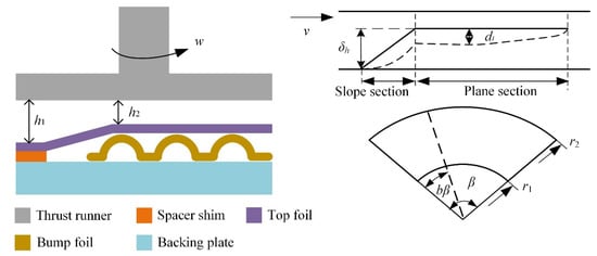
Figure 4.
Structure and operation principle of GFTB.
Otherwise, modeling of the connecting groove between pads is also considered in the present work, which is shown in Figure 2b. The groove is divided into exactly the same two parts, which are connected in the flat section and the slope section of the gas film, respectively. The reason for this modeling form is that the two rotational periodic symmetry boundaries require the geometry shape and dimension to be exactly the same, to enable the computational data to be transferred completely.
Due to the fact that the magnitude of load-carrying capacity is directly affected by the minimum film thickness presented in the computational domain model, and the fact that the change in the thickness needs to deal with the geometry model again, it is difficult to parameterize the micron-scale gas film thickness, and the geometry model needs to be cleaned up and patched in the preprocessing step. Thus, the film thickness is set constant to analyze the performance of the GFTBs conveniently, and the loadcarrying capacity discussed here is also not the maximum value of foil structures.
2.3. Modeling of Bearing Structure
The computational domain is shown in Figure 2; the backing plate and spacer shim material usually use structural steel, which is assumed for a fixed rigid body domain, and the foil material is a nickel–chromium alloy which has great elastic deformation properties. Thus, the main deformation components of GFTBs are the top foil and bump foil under high-speed gas pressure. The deformation of foils follows Hooke’s law written as
where σ is the second-order stress tensor, and ε is the second-order strain tensor, which is related to the deformation and C is the fourth-order elasticity tensor. The equilibrium equation of steady state is given by Newton’s second law as follows,
where fV is the body force per unit deformed volume, and is the gradient operators taken with respect to the spatial coordinates.
Meanwhile, the contact between bump foil and backing plate, as well as between the bump foil and the top foil, has a significant influence on the foil deformation too. The penalty function method is used in the multi-physics coupled contact, which is equivalent to adding a spring boundary load between the surfaces to complete the virtual contact. Furthermore, to implement loading gradually, a loading function can be defined here. In this contact model, in addition to considering the penalty type normal force, a Coulomb friction law is also added to refine the model, with a friction coefficient μ = 0.1 and a friction penalty factor ft = 0.1. The selection of the friction coefficient value is based on the values used frequently in similar GFTBs simulations or experiments analysis from other literatures, e.g., Refs. [25,26].
The contact pairs in this structure domain are shown in Figure 5. On the settings of the contact pairs, the easily deformable surface and the surface with a small bending radius are set as the target surfaces, and the surface that is difficult to deform is set as the source surface. Furthermore, the rigid body must be the source surface. The mesh size of the target surface needs to be smaller. In general, it is half the size of the source face mesh. In addition, the contact penalty factor fp could control the convergence speed, and stability, and increasing the penalty factor can speed up the solution process, but it is also easy to cause the solution to diverge. The range of the factor is set to (0.05, 0.2) in this structure model.
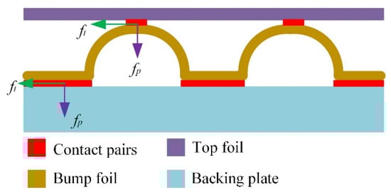
Figure 5.
Schematic diagram of contact pairs.
2.4. Modeling of Heat Transfer
The only heat source in this computational model comes from the shear stress of the fluid film, which is solved with the three-dimensional energy equation. After the heat flux being generated in the gas film, it flows to the rotor disk side and the thrust-bearing side through heat in conduction. On the rotor disk side, the heat flux spreads out through natural convection. On the thrust-bearing side, the heat flux from the top foil is conducted to the bump foil and then to the backing plate through thermal contact. Meanwhile, the heat flux is also conducted to the base plate through the air between foils, and finally it spreads out from backing plate surface to environment through natural convection. The heat flux transfer schematic is shown in Figure 6. The heat conduction and heat convection equations are as follows,
where q is the heat flux by conduction (W/m2), k is the thermal conductivity (W/(m·K)), is the temperature gradient (K), ρ is the density (kg/m3), Cp is the specific heat capacity at constant stress (J/(kg·K)), T is the absolute temperature (K), and Q contains heat sources other than viscous dissipation (W/m3).
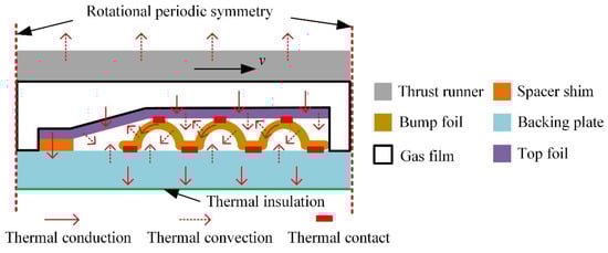
Figure 6.
Heat flux transfer schematic.
Thermal contact is an important heat transfer route in this TEHD model, in which contact conductivity hc (W/(m2·K)) is mainly influenced by the surface roughness and contact pressure coupled with structural mechanics generally, and thermal conductivity of air gap hg (W/(m2·K)) depends on the medium properties of the gap space. The region of thermal contact pairs is the same as the region of the structure contact pairs mentioned in the last section, as shown in Figure 4.
2.5. Boundary Condition
2.5.1. Fluid Flow
As Figure 7 presents, the bottom boundary of the fluid flow domain is set as a stationary wall, and the upper boundary of the fluid flow domain is assumed to be a moving wall at a constant angular velocity v = ω × r. All stationary walls and moving solid walls are assumed to be no-slip conditions and impermeable. The left and right sides of the fluid flow domain are set as the rotational periodic symmetry boundaries.
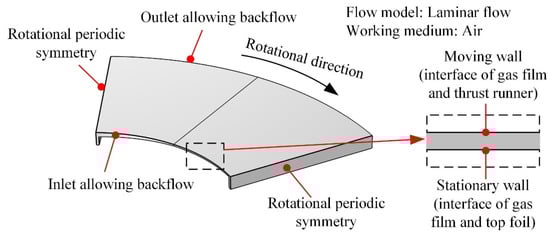
Figure 7.
The boundary conditions of fluid flow.
The inlet and outlet surfaces of the fluid flow domain are always considered as pressure inlet and pressure outlet, and the pressure is assumed to be constant at the same value p0 (gauge pressure). In most of the numerical simulations p0 = 0 (Pa), there are other scholars, like Gen Fu et al. [16], who assumed p0 to be slightly higher than ambient pressure. The pressure inlet and pressure outlet do not suppress reverse flows of the boundaries, which allows the simulation results of the gas film flow to obtain a more realistic flow trend.
In the present study, the fully developed flow boundary condition is applied to the inlet and outlet of channel, and this type of boundary condition has been applied to the inlet boundary of a two-pass rectangular smooth channel in which velocity and temperature are mapped from the outlet of a periodic segment [27]. Qahtan [28] applied a fully developed flow boundary condition at the inlet channel of a wavy channel partially filled with a porous layer, wherein the velocities and turbulent quantities were calculated separately. Batista [29] applied the fully developed water inlet boundary condition in a crossflow air-to-water fin-and-tube heat exchanger, and compared it with uniform flow velocity and temperature profiles; its numerical results coincide well with experimental measurements. Compared to traditional inlet and outlet pressure boundaries, a fully developed flow boundary could obtain more accurate numerical results, which is also consistent with the continuous property of fluid flow and has better convergence performance in CFD.
2.5.2. Structure Deformation
For the structure domain, as presented in Figure 2a, boundary conditions are set as follows. The leading edge of the top foil and bump foil are regarded as fixed boundaries, and other edges are set as free; the left and right sides of the backing plate are set as rotational periodic symmetry boundaries, and the backing plate and spacer shim are regarded as fixed rigid bodies.
2.5.3. Thermal Transfer
The thermal computational domain contains the whole fluid flow and structure domain, as shown in Figure 6. The rotational periodic symmetry boundaries are the same as those two domains above. The inlet and outlet boundaries of the fluid flow domain are set as open boundaries. The upper side of the top foil is coupled with the bottom side of fluid flow, which results in a continuous temperature field. Besides the thermal contact region, the rotor disk side and all the rest of the solid surfaces are set as heat convection boundaries.
2.6. Mesh
Moving mesh technology is applied in this TEHD model, and the whole fluid flow domain is set as a moving mesh domain. During the calculation process, as the structure deformation is coupled, the shape of the mesh is adapted accordingly. Due to the fact that the velocity changes faster in the film thickness direction (axial direction) than that in the circumferential and radial directions, the layer number of the mesh in the direction of film thickness becomes more important than in the other two directions. To improve calculation efficiency with guaranteed accuracy, the convergence of mesh with the verify method described in Ref. [30] is illustrated in Figure 8. It is concluded that the simulation results converge when the mesh layer in the direction of gas film is increased to six and ensures the number of the mesh is sufficient in the circumferential and radial directions, which is reliable enough to applied to the following analysis. The fluid region is structured to be meshed through mesh control domain methods with approximately 520,000 cells, and the structure region is meshed with approximately 50,000 cells. Almost all the fluid and structural domains are gridded by structured meshes, i.e., hexahedral meshes; only the bump foil part is gridded by unstructured meshes, i.e., tetrahedral meshes. The structured mesh can conveniently achieve the boundary fitting, which is suitable for the calculation of fluid and surface stress concentrations, etc. It is generated quickly and with good quality, but it is only applicable to the regular shape of the structure. Generally speaking, the computational results of structured meshes converge more easily than unstructured meshes, and unstructured meshes have structural adaptability.
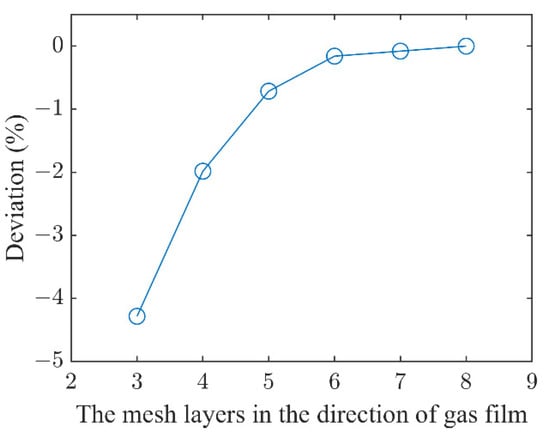
Figure 8.
Mesh convergence verification of CFD simulation.
2.7. Validation of CFD Model
Figure 9 shows the simulation results of the fluid flow trend compared with the results from Ref. [8], which all indicate clearly that most of the flow leaks out at the slope region side of the film. Figure 9b applied the normal pressure inlet and outlet boundary condition, while Figure 9c applied the fully developed pressure inlet and outlet boundary condition. The overall trend is roughly the same, but the flow becomes more complex at the inside slope region of the gas film.
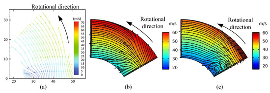
Figure 9.
Flow trend of gas film. (a) Results from Ref. [8]. (b) CFD simulation with normal pressure boundary. (c) CFD simulation with fully developed pressure boundary.
The fluid structure coupled simulation results in the CFD model are compared with the results calculated by the numerical simulation method mentioned in Ref. [31], using the GFTBs geometry and operating parameters in Table 1. As Figure 10 shows, there is a positive linear trend in the relationship between bearing load-carrying capacity and rotational speed in both numerical results and CFD results. Meanwhile, the CFD results are higher than the results of the numerical simulation, which might be caused by the simplifications of the Reynolds equation and structure deformation in the numerical method. Therefore, the CFD model built in this study is reliable for subsequent analysis of the performances of GFTBs.
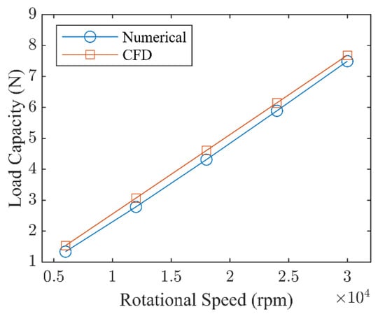
Figure 10.
The relationship between load carrying capacity and rotational speed (The numerical simulation method was mentioned in Liu et al. [31]).
3. Results and Discussion
Table 1 lists the bearing structure and operating parameters used in the present simulation.

Table 1.
GFTB structure and operating parameters.
Table 1.
GFTB structure and operating parameters.
| Parameters | Values |
|---|---|
| Bearing inner radius r1 (mm) | 10 |
| Bearing outer radius r2 (mm) | 20 |
| Pitch ratio b | 0.5 |
| Number of pads N | 6 |
| Pad arc degree β (°) | 58 |
| Slope height δh (μm) | 20 |
| Minimum gas film thickness h2 (μm) | 10 |
| Top foil thickness td (mm) | 0.1 |
| Bump foil thickness tb, height hb (mm) | 0.1, 0.4 |
| Bump half length l, Bump pitch s (mm) | 0.3, 1 |
| Elastic modulus Eb (GPa) | 210 |
| Poisson’s ratio vb | 0.3 |
| Foil density ρb (kg/m3) | 8240 |
| Foil thermal conductivity kt (W/K·m) | 16.9 |
| Backing plate thickness tz (mm) | 1 |
| Environment temperature T0 (°C) | 20 |
| Nature convection of solid surface kn (W/K·m) | 12 |
| Friction coefficient μ | 0.1 |
| Penalty factor fp | (0.05,0.2) |
3.1. Fluid-Structure Coupled Simulation
Figure 11 illustrates the pressure distribution of gas film obtained by the fluid structure coupled simulation, with a rotational speed of 30,000 rpm for different average pressures p0 (Pa) at inlet and outlet boundaries which are all set as fully developed flow. Figure 11a shows the pressure distribution at p0 = 6000 Pa. Along the circumferential direction, the pressure increases rapidly from the groove symmetry boundaries at inlet, and reaches the maximum value when the gas flow reaches the junction of slope section and flat section. Then, it decreases quickly to the same pressure value with the inlet when it reaches groove symmetry boundary at outlet. In the radial direction, the high-pressure area is concentrated near the connecting line of the slope section and the flat section and close to the outer radius region. The pressure in the area closest to the inlet and outlet boundaries is close to the atmospheric pressure, but the boundary pressure near the highest pressure at the outer radius is slightly higher than atmospheric pressure due to the fully developed flow.
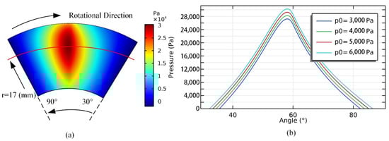
Figure 11.
Pressure distribution of the gas film. (a) p0 = 6000 Pa; (b) pressure along the circumferential sectional line at the highest pressure point where r = 17 mm, with different boundary pressure.
Due to the pressure distribution discipline with different inlet and outlet average boundary pressure are the same, as described in the previous paragraph. To show the difference in their numerical values more clearly, Figure 11b presents the pressure along the circumferential sectional line at the pressure highest point of the gas film where r = 17 mm, approximately, with different inlet and outlet average boundary pressures. It can be seen that the pressure increases almost uniformly in the form of an arithmetic progression on this line as the boundary pressure increases.
Figure 12 shows the deformations of top foil with different average boundary pressures at inlet and outlet listed in Figure 11b. The maximum top foil deformation occurs at the outer radius edge of the slope section in most instances, whereas the boundary pressure is high enough, as shown in Figure 12b–d, which is the consequence of no bump foil support under the slope section. However, in the case of insufficient boundary pressure, as shown in Figure 12a, the maximum top foil deformation appears at the outer radius edge near the trailing edge, which is the location that often first appears as an abrasion. Hence, the initial average boundary pressure has a significant effect on the deformation of the top foil.
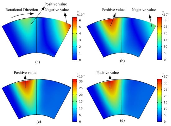
Figure 12.
Deformation of top foil (positive value means the deform direction is the same with the pressure). (a) p0 = 3000 Pa; (b) p0 = 4000 Pa; (c) p0 = 5000 Pa; (d) p0 = 6000 Pa.
Under the action of the pressure transmitted by top foil, the deformation of the bump foil as a support structure was also investigated, as shown in Figure 13. When the inlet and outlet average boundary pressure is relatively small, the free end of the bump foil will be upturned, and the deformation is more significant than the front bumps, which might be caused by the peak pressure of gas film acting on the front bumps (combining the pressure distribution in Figure 11). The leverage of the force causes the rear bump to upturn, and the pressure of the trailing edge is not large enough to push it down, as Figure 13a shows. When the inlet and outlet average boundary pressure increases, the upturn displacement decreases gradually, and the first bump at the region of maximum pressure is pushed downwards more evidently; meanwhile, the following two bumps (2nd and 3rd) will be deformed upward under the leverage of the force. The last two bumps (4th and 5th) are pushed downwards by the top foil under the large boundary pressure.
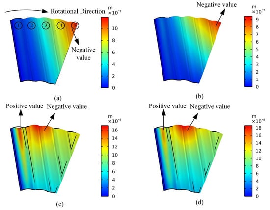
Figure 13.
Deformation of bump foil (positive value means the deform direction is the same with the pressure). (a) p0 = 3000 Pa; (b) p0 = 4000 Pa; (c) p0 = 5000 Pa; (d) p0 = 6000 Pa.
The effect of rotational speed on the pressure of GFTB is also investigated, as shown in Figure 14. The pressure distributions along the circumferential sectional line is at the highest pressure point where r = 17 mm. The results indicates that the pressure rise rate increases as the rotational speed increases and the positions of the peak pressures does not change with the rotational speed.
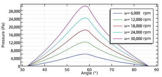
Figure 14.
Pressure distribution along the circumferential sectional line where r = 17 mm, p0 = 6000 Pa, under different rotational speeds.
3.2. Fluid-Structure-Thermal Coupled Simulation
The thermal investigation is conducted to analyze the effect of increased boundary pressure and rotational speed in this section. Under the rotational speed of 30,000 rpm, Figure 15 shows the pressure along the circumferential sectional line at highest pressure point where r = 17 mm, with different boundary pressures. Compared with that result in Figure 11b, it has a higher overall pressure curve when considering the thermal influences.
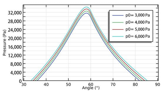
Figure 15.
Pressure distribution along the circumferential sectional line at the highest pressure point where r = 17 (mm), with different boundary pressure in the TEHD model.
Correspondingly, the load-carrying capacity of GFTBs would also change with the different boundary pressures and rotational speeds, as illustrated in Figure 16. It can be concluded that the load-carrying capacity tends to increase linearly with the growth of rotational speed in the isothermal model; meanwhile, the increase is more pronounced at larger boundary pressure p0. When considering the influence of temperature, the load-carrying capacity of GFTBs can be improved to some extent compared with the isothermal model, and as the rotational speed increased, the improvement of the load capacity also rose. It is an approximately ten percent increase where rotational speed is 30,000 (rpm), which may be caused by the increase in temperature. Figure 17 shows the maximum temperature influenced by boundary pressures. The change of boundary pressure generally causes a minor impact on the maximum temperature of GFTB components (maximum about 6%). The temperature of bump foil and backing plate rise a few degrees when the boundary pressure increases. On the other hand, the temperature of gas film and top foil decreased by a few degrees, which might be caused by the fully developed boundary condition that accelerates the heat exchange of boundaries.
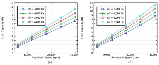
Figure 16.
Load-carrying capacities under different boundary pressures and rotational speeds: (a) Isothermal model. (b) TEHD model.
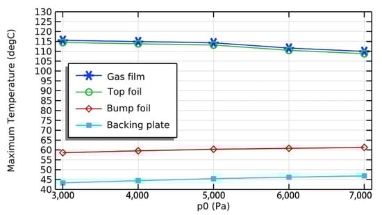
Figure 17.
The maximum temperature change of GFTB components with different boundary pressures.
In comparison, as shown in Figure 18, the rotational speed significantly influences the maximum temperature of GFTB due to the heat generated within the gas film by viscous shear effect, which is directly related to the gradients of fluid velocity in gas film thickness direction. The temperatures of gas film and top foil increase rapidly with the increase of rotational speed, and the temperatures of bump foil and backing plate also increase at a relatively lower rate. This is because when the heat flow transfers from gas film to the top foil, bump foil, and backing plate, on one hand the thermal contact resistant reduces the heat transfer efficiency and on the other part of the heat is lost through natural convection from structure surfaces.
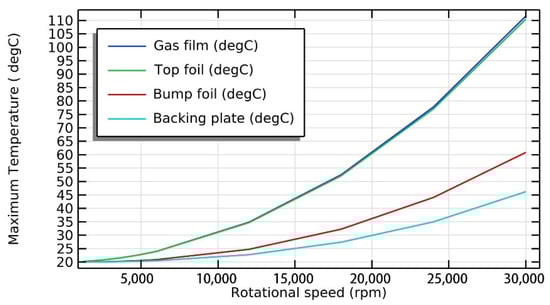
Figure 18.
The maximum temperature of GFTB components with different rotational speeds.
The characteristics of multiple fields are obtained in Figure 19 and Figure 20. The gas film pressures are presented in Figure 19. The left side is under the rotational speed of 6000 rpm, and the right side is under the rotational speed of 30,000 rpm, and both have the inlet and outlet boundary pressure of p0 = 6000 Pa. Correspondingly, Figure 20 presents the characteristic temperature distribution of GFTB on the same condition. It can be seen from Figure 20a,b that the temperature is distributed evenly in the thin gas film and accumulated at the outer radial trailing edge, which is because the rotor disk is simplified as a natural convection. Moreover, the lowest temperature region appears at the groove of the inner and outer radial boundary where the ambient air enters, which means the inner and outer radial boundaries of the groove are the actual gas inlet boundaries, and the rest of pressure boundaries are the actual gas outlet boundaries. This is due to the fact that the backflow is not suppressed at the pressure inlet and outlet boundaries.
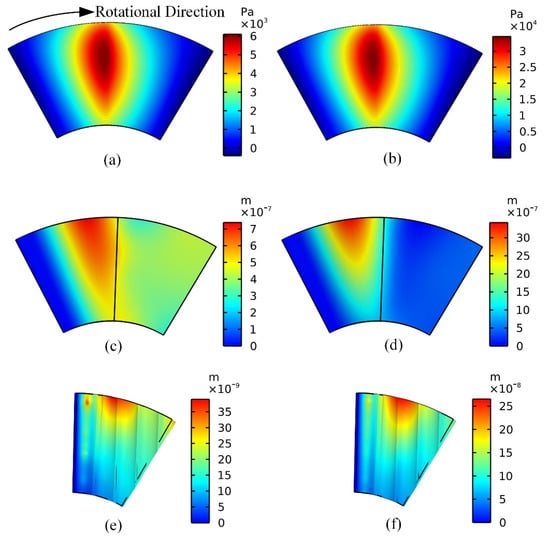
Figure 19.
Characteristic static performance of GFTB in ω = 6000 rpm (left side) and ω = 30,000 rpm (right side). (a,b) Pressure distribution. (c,d) Deformation of top foil. (e,f) Deformation of bump foil.
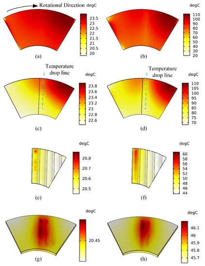
Figure 20.
Characteristic temperature distribution of GFTB in ω = 6000 rpm (left side) and ω = 30,000 rpm (right side). (a,b) Gas film. (c,d) Top foil. (e,f) Bump foil. (g,h) Backing plate.
The temperature distributions of top foil at different rotational speeds are similar. Figure 20c,d show that the highest temperature region appears at the outer radial trailing edge of top foil, which is the same as the results in Ref. [11]. Considering the fluid flow diagram in Figure 9c, most of the flow leaks out at the slope region of the gas film, which also takes away some heat leading to a low-temperature area at the slope section of top foil.
The temperature rise of bump foil and backing plate is mainly due to thermal contacts (i.e., bump foil/top foil and bump foil/backing plate), which contain air gap heat conduction and a diffuse radiation of gray bodies between parallel planes associated with surface roughness, contact pressure, air gap properties, etc. It can be clearly seen that the heat transfer through the contact pairs in Figure 20e–h, combines the pressure distribution and foil deformation in Figure 19, and the heat transfer efficiency of the contact pairs are greatly affected by the contact pressure. There is also a clear line of a temperature drop on the top foil, at the contact pair coincidence area where the heat transfer efficiency is most pronounced especially in Figure 20d.
The simulated top foil temperature is compared with other similar research results as shown in Figure 21. It can be seen that the temperature distribution trends are similar, and the temperature peak both appears at the trailing edge near out radius, but the overall temperature distributions in reference [11] is relatively higher than the results in this work, which is mainly caused by the facts that the rotor speed in reference is much higher, and the size of the bearing is also relatively larger. Thus, the TEHD model built in present work is reasonable for the analysis.
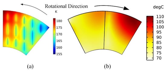
Figure 21.
Top foil temperature comparison with Ref. [11]. (a) Top foil temperature increase for a rotor speed of 120 krpm in Ref. [11]. (b) Top foil temperature distribution in present model.
4. Conclusions
A detailed three-dimensional thermo-elastic-hydrodynamic (TEHD) coupling model has been developed to analyze the fluid-structure-thermal performance of bump-type GFTBs in the current study. The fully developed flow boundary conditions were applied in this model. The effects of boundary pressure, and rotational speed were investigated. Moreover, friction and thermal contacts between bump foil and top foil and between bump foil and backing plate were considered. The main conclusions are obtained as follows.
- The increasing of boundary pressure could improve the overall pressure distribution of the gas film and also has a significant effect on the deformation of top foil. When the boundary pressure is too low, the trailing edge of the top foil will be deformed upward at the very beginning.
- The temperature rises as a consequence of viscous dissipation of high-speed fluid flow. Hence the rotational speed has the most direct effect, especially for the gas film and top foil. The temperature distributions of all components of GFTBs have explained the mechanisms of heat transfer. The temperature peak of the top foil appears at the trailing edge near outer radius. The heat is conducted to the bump foil and backing plate through the contact pairs, which are affected by the contact pressure.
- According to the temperature distribution and the speed streamline of gas film, the actual route of gas flow can be inferred that the ambient air with lower temperature enters the gas film from the groove of inner and outer radial channels. Most of the flow leaks out at the slope region and takes away some of the heat, which leads to a low-temperature region. The generated heat accumulates at the flat section and reaches the maximum temperature, finally mixing with ambient air that enters from the next groove.
- Temperature is a significant factor that cannot be ignored when analyzing the GFTB performance. The load-carrying capacity would be improved to some degree in the TEHD model compared with the isothermal model, especially when the rotational speed increases, reaching an approximately ten percent improvement at the rotational speed of 30,000 rpm in this case.
Author Contributions
Conceptualization, J.D. and X.L.; methodology, X.L.; software, X.L.; validation, X.L., C.L. and J.D.; formal analysis, C.L.; investigation, X.L.; resources, C.L. and J.D.; data curation, X.L.; writing—original draft preparation, X.L.; writing—review and editing, X.L. and C.L.; visualization, X.L.; supervision, J.D.; project administration, C.L.; funding acquisition, C.L. and J.D. All authors have read and agreed to the published version of the manuscript.
Funding
This research was funded by the National Natural Science Foundation of China (Grant No. U2141210), (Grant No. 52005126).
Data Availability Statement
The data presented in this study are available on reasonable request from the corresponding author.
Conflicts of Interest
The authors declare no conflict of interest.
References
- Agrawal, G.L. Foil Air/Gas Bearing Technology—An Overview; American Society of Mechanical Engineers: Orlando, FL, USA, 1997. [Google Scholar]
- San Andrés, L.; Kim, T.H. Analysis of gas foil bearings integrating FE top foil models. Tribol. Int. 2009, 42, 111–120. [Google Scholar] [CrossRef]
- Salehi, M.; Swanson, E.; Heshmat, H. Thermal Features of Compliant Foil Bearings—Theory and Experiments. J. Tribol. 2001, 123, 566–571. [Google Scholar] [CrossRef]
- Peng, Z.C.; Khonsari, M.M. A Thermohydrodynamic Analysis of Foil Journal Bearings. J. Tribol. 2006, 128, 534–541. [Google Scholar] [CrossRef]
- Paulsen, B.T.; Morosi, S.; Santos, I.F. Static, Dynamic, and Thermal Properties of Compressible Fluid Film Journal Bearings. Tribol. Trans. 2011, 54, 282–299. [Google Scholar] [CrossRef]
- Lee, D.; Kim, D. Three-Dimensional Thermohydrodynamic Analyses of Rayleigh Step Air Foil Thrust Bearing with Radially Arranged Bump Foils. Tribol. Trans. 2011, 54, 432–448. [Google Scholar] [CrossRef]
- Hu, H.; Feng, M.; Ren, T. Study on the performance of gas foil thrust bearings with stacked bump foils. Ind. Lubr. Tribol. 2020. ahead-of-print. [Google Scholar] [CrossRef]
- Gad, A.M.; Kaneko, S. Fluid Flow and Thermal Features of Gas Foil Thrust Bearings at Moderate Operating Temperatures; Springer: Cham, Switzerland, 2015. [Google Scholar]
- Kai, F.; Kaneko, S. A Thermohydrodynamic Sparse Mesh Model of Bump-Type Foil Bearings. J. Eng. Gas Turbines Power 2013, 135, 022501. [Google Scholar]
- Sim, K.; Kim, D. Thermohydrodynamic Analysis of Compliant Flexure Pivot Tilting Pad Gas Bearings. J. Eng. Gas Turbines Power 2008, 130, 460–466. [Google Scholar] [CrossRef]
- Rieken, M.; Mahner, M.; Schweizer, B. Thermal Optimization of Air Foil Thrust Bearings Using Different Foil Materials. J. Turbomach. 2020, 142, 101003. [Google Scholar] [CrossRef]
- Lehn, A.; Mahner, M.; Schweizer, B. A thermo-elasto-hydrodynamic model for air foil thrust bearings including self-induced convective cooling of the rotor disk and thermal runaway. Tribol. Int. 2017, 119, 281–298. [Google Scholar] [CrossRef]
- Xu, F.; Kim, D. Three-Dimensional Turbulent Thermo-Elastohydrodynamic Analyses of Hybrid Thrust Foil Bearings Using Real Gas Model. In Proceedings of the Asme Turbo Expo: Turbomachinery Technical Conference & Exposition, Seoul, South Korea, 13–17 June 2016; p. V07BT31A030. [Google Scholar]
- Aksoy, S.; Aksit, M.F. A fully coupled 3D thermo-elastohydrodynamics model for a bump-type compliant foil journal bearing. Tribol. Int. 2015, 82, 110–122. [Google Scholar] [CrossRef]
- Xu, Z.; Ji, F.; Zhou, Y.; Wu, F.; Ding, S. Modelling on Predicting Pressure Distribution and Capacity of Foil Thrust Bearing. In Proceedings of the ASME 2018 International Mechanical Engineering Congress and Exposition, Pittsburgh, PA, USA, 9–15 November 2018. [Google Scholar]
- Fu, G.; Untaroiu, A.; Swanson, E. Effect of Foil Geometry on the Static Performance of Thrust Foil Bearings. J. Eng. Gas Turbines Power 2018, 140, 082502. [Google Scholar] [CrossRef]
- Untaroiu, A.; Fu, G. Surrogate Model Based Optimization for Chevron Foil Thrust Bearing. In Proceedings of the ASME Turbo Expo 2019, Turbomachinery Technical Conference and Exposition, Phoenix, AZ, USA, 17–21 June 2019. [Google Scholar]
- Qin, K.; Jahn, I.H.; Jacobs, P.A. Effect of Operating Conditions on the Elasto-Hydrodynamic Performance of Foil Thrust Bearings for Supercritical CO2 Cycles. J. Eng. Gas Turbines Power 2016, 139, 042505. [Google Scholar] [CrossRef]
- Qin, K.; Gollan, R.J.; Jahn, I.H. Application of a wall function to simulate turbulent flows in foil bearings at high rotational speeds. Tribol. Int. 2017, 115, 546–556. [Google Scholar] [CrossRef]
- Qin, K.; Jacobs, P.A.; Keep, J.A.; Li, D.; Jahn, I.H. A fluid-structure-thermal model for bump-type foil thrust bearings. Tribol. Int. 2018, 121, 481–491. [Google Scholar] [CrossRef]
- Kim, D.; Ki, J.; Kim, Y.; Ahn, K. Extended three-dimensional thermo-hydrodynamic model of radial foil bearing: Case studies on thermal behaviors and dynamic characteristics in gas turbine simulator. J. Eng. Gas Turbines Power 2012, 134, 052501. [Google Scholar] [CrossRef]
- Ravikovich, Y.; Ermilov, Y.; Pugachev, A.; Matushkin, A.; Kholobtsev, D. Prediction of stiffness coefficients for foil air bearings to perform rotordynamic analysis of turbomachinery. In Proceedings of the 9th IFToMM International Conference on Rotor Dynamics; Springer: Cham, Switzerland, 2015; pp. 1277–1288. [Google Scholar]
- Supreeth, S.; Ravikumar, R.; Raju, T.; Dharshan, K. Foil stiffness optimization of a gas lubricated thrust foil bearing in enhancing load carrying capability. Mater. Today Proc. 2022, 52, 1479–1487. [Google Scholar] [CrossRef]
- Yu, T.-Y.; Wang, P.-J. Simulation and Experimental Verification of Dynamic Characteristics on Gas Foil Thrust Bearings Based on Multi-Physics Three-Dimensional Computer Aided Engineering Methods. Lubricants 2022, 10, 222. [Google Scholar] [CrossRef]
- Rubio, D.; San Andres, L. Structural stiffness, dry friction coefficient, and equivalent viscous damping in a bump-type foil gas bearing. J. Eng. Gas Turbines Power 2007, 129, 494–502. [Google Scholar] [CrossRef]
- Gad, A.M.; Kaneko, S. A new structural stiffness model for bump-type foil bearings: Application to generation II gas lubricated foil thrust bearing. J. Tribol. 2014, 136, 041701. [Google Scholar] [CrossRef]
- Siddique, W.; El-Gabry, L.; Shevchuk, I.V.; Hushmandi, N.B.; Fransson, T.H. Flow structure, heat transfer and pressure drop in varying aspect ratio two-pass rectangular smooth channels. Heat Mass Transf. 2011, 48, 735–748. [Google Scholar] [CrossRef]
- Al-Aabidy, Q.; Alhusseny, A.; Al-zurfi, N. Numerical investigation of turbulent flow in a wavy channel partially filled with a porous layer. Int. J. Heat Mass Transf. 2021, 174, 121327. [Google Scholar] [CrossRef]
- Batista, J.; Trp, A.; Lenic, K. Experimentally validated numerical modeling of heat transfer in crossflow air-to-water fin-and-tube heat exchanger. Appl. Therm. Eng. 2022, 212, 118528. [Google Scholar] [CrossRef]
- Zhuang, H.; Ding, J.; Chen, P.; Chang, Y.; Zeng, X.; Yang, H.; Liu, X.; Wei, W. Numerical Study on Static and Dynamic Performances of a Double-Pad Annular Inherently Compensated Aerostatic Thrust Bearing. J. Tribol. 2019, 141, 051701. [Google Scholar] [CrossRef]
- Liu, X.; Li, C.; Du, J.; Nan, G. Thermal Characteristics Study of the Bump Foil Thrust Gas Bearing. Appl. Sci. 2021, 11, 4311. [Google Scholar] [CrossRef]
Publisher’s Note: MDPI stays neutral with regard to jurisdictional claims in published maps and institutional affiliations. |
© 2022 by the authors. Licensee MDPI, Basel, Switzerland. This article is an open access article distributed under the terms and conditions of the Creative Commons Attribution (CC BY) license (https://creativecommons.org/licenses/by/4.0/).