Experimental Measurement of Ice-Curling Stone Friction Coefficient Based on Computer Vision Technology: A Case Study of “Ice Cube” for 2022 Beijing Winter Olympics

Abstract

In the curling sport, the coefficient of friction between the curling stone and pebbled ice is crucial to predict the motion trajectory. However, the theoretical and experimental investigations on stone–ice friction are limited, mainly due to the limitations of the field measurement techniques and the inadequacy of the experimental data from professional curling rinks. In this paper, on-site measurement of the stone–ice friction coefficient in a prefabricated ice rink for the Beijing Winter Olympics curling event was carried out based on computer vision technology. Firstly, a procedure to determine the location of the curling stone was proposed using YOLO-V3 (You Only Look Once, Version 3) deep neural networks and the CSRT Object tracking algorithm. Video data was recorded during the curling stone throwing experiments, and the friction coefficient was extracted. Furthermore, the influence of the sliding velocity on the friction coefficient was discussed. Comparison with published experimental data and models and verification of the obtained results, using a sensor-based method, were conducted. Results show that the coefficient of friction (ranging from 0.006 to 0.016) decreased with increasing sliding velocity, due to the presence of a liquid-like layer. Our obtained results were consistent with the literature data and the friction model of Lozowski. In addition, the experimental results of the computer vision technique method and the accelerometer sensor method showed remarkable agreement, supporting the accuracy and reliability of our proposed measurement procedure based on deep learning.

1. Introduction

Curling, also known as “chess on ice”, is a widespread winter sport combining strategy and skill, and it requires a high level of concentration and precision [1,2,3]. In recent years, especially following the success of the 2022 Winter Olympics in Beijing, the sport of curling has attracted increasing interest from around the world [4].

In the curling game, the rotating stone following a curled trajectory, rather than keeping a straight trajectory, is a well-acknowledged phenomenon. For a stone sliding with a clockwise rotational velocity, a transverse motion component on the right-hand side will develop, and vice versa [5,6]. For almost a century, many attempts have been made by scholars to explain the curling motion. For instance, forward–backward asymmetry friction over the running band of curling stones was adopted by many researchers to predict the observed curling behavior. According to the different mechanisms explaining the asymmetry, the forward–backward asymmetry friction models can be divided into six models, that is, the pressure difference model, the water layer model, the snowplow model, the evaporation-abrasion model, the scratch-guiding model, and the edge model [3,7,8,9,10,11]. Recently, the mechanism for getting the stone to follow a curved trajectory has been investigated using a pivot–slide-based model [12,13] and a split friction model by Ziegler [14]. In short, although several models have been proposed in the surveyed literature, the mechanism is still under scientific debate. This is primarily because of the complicated motion process and a lack of sufficiently precise observation data [5,15].

It is well known that friction and motion are largely influenced by the characteristics of the stone–ice contact surface. The curling stone (Figure 1) is specially made of about 20 kg of granite rock with a rough bottom. Through a raised annulus with a width of about 6 mm and a diameter of about 120 mm, i.e., a running band/RB, the bottom of the curling stone is in contact with the curling ice. There are many small protrusions, called pebbles, on the surface of the curling ice, roughly 10⁴ pebbles per square meter of ice, that reduce the curling distance [16,17]. The pebbles are produced by technicians spraying purified water droplets onto the initially flat ice surface. The pebble sizes, with an average height of 1–2 mm and a diameter of 3–10 mm, are controlled by the size of the spray hole. As only about 10–100 pebbles are in constant contact with the curling stone RB, the actual pressure magnitude exerted by the stone on the pebbles is considerable, about 0.4–8.1 MPa [18]. The multiple features of these contact surfaces comprehensively affect the movement of the stone and increase the fun of the game. In 2020, Kameda et al. [10] pointed out that the curl distance was primarily determined by the stone RB (surface roughness and area), instead of the ice surface conditions. The curl phenomenon can be regarded as the result of multiple physical mechanisms working together, and the influence of these mechanisms can be expressed by the stone–ice friction coefficient [18].

Studies on the stone–ice friction coefficient include experiment-based research and theory-based research. For experiments, Penner [19] measured friction by manually dragging a curling rock along the ice of a local curling rink at a constant velocity, and recorded the required force. However, the coefficient of kinetic friction at velocities greater than approximately 1 m/s and less than 0.15 m/s could not be obtained using this approach. Furthermore, Nyberg et al. [20] designed a special device combining an electric motor and force gauge to measure the friction force of a curling stone sliding over the ice. As shown in Figure 2, the sliding velocity was improved in comparison with the measurement method adopted by Penner [19]. In their study, the dependence of the stone–ice friction coefficient on the sliding speed and roughness of the curling stone was investigated. In terms of the theoretical research, although many theoretical models of kinetic ice friction have been proposed [21,22,23,24], no adequate model has been developed and validated for curling stones. One of the limited models was presented by Penner [19]. In this research, the calculation of the coefficient of kinetic friction was from the perspective of energy transfer, rather than the actual physical mechanism between the interacting interfaces. In addition, using the ice skating friction derivation method [25], Lozowski et al. [26] developed a numerical model of the stone–ice friction coefficient, based on thermodynamic equilibrium. The effects of multi-parameters of both the ice and curling stone, such as geometrical parameters, thermal parameters, ice hardness, and stone sliding velocity, were incorporated in the model.

In summary, the investigation of friction is limited mainly by the limitations of on-site measurement technology and insufficient experimental data from professional curling rinks. In recent years, artificial intelligence methods and strategies have been increasingly developed to explore the complex tribological characteristics [27,28]. Computer vision technology based on deep learning provides an insight into the motion trajectory, and can be used as an effective measurement technique. With the progress of artificial intelligence technology, deep-learning-based object detection methods showing impressive performance in speed, accuracy, and automaticity, and have been extensively applied in scenarios, such as structural health monitoring [29,30,31]. The object detection algorithms based on deep learning mainly include one-stage and two-stage algorithms. You Only Look Once/YOLO [32] is a one-stage object detection algorithm with real-time object recognition and localization capabilities through a convolutional neural network.

To better understand the friction coefficient of a stone sliding on ice in the “Ice Cube” rink designed for the 2022 Beijing Winter Olympics, this study adopted the YOLO-V3 model and CSRT object tracking algorithm with a good balance in speed and precision to perform curling stone tracking and recognition. The main contributions in this paper are summarized as follows:

(1)

The friction coefficient of a curling stone sliding on pebbled ice in an actual rink for the Beijing Winter Olympics was obtained, based on on-site measurement.

(2)

A procedure to determine the location of the curling stone was proposed, based on YOLO-V3 deep neural networks and the CSRT tracker. The method may be further applied to actual competitions without the ethical issues of competition, which may contribute to revealing the complex friction mechanism of stone–ice.

(3)

A curling stone dataset containing 1000 images was created to supply the data for the study of curling stone object recognition.

The remainder of the paper is organized as follows. In the second part, the deep-learning-based methodologies for determining curling stone locations are proposed. Descriptions of the investigated curling rink, measurement methods, and data processing are presented in the third part. In the fourth part, the effects of sliding velocity on friction, calculation model assessment, and accelerometer-based experimental verification are discussed. Finally, conclusions are drawn from the experimental results and analyses.

2. Methodologies

2.1. Image Dataset Description

2.1.1. Video Data Acquisition

Videos were recorded with a high-definition camera with a resolution of 3840 × 2160 pixels at a rate of 60 frames per second.

2.1.2. Image Acquisition, Annotation and Dataset Production

In this paper, images were first extracted frame-by-frame from the video stream. Secondly, manual object localization, namely, the position identified by creating a bounding box around the region of interest/ROI, i.e., the curling stone in this study, was conducted for 1000 images. Finally, the annotated images were converted to the YOLO format to train using the YOLO-V3 deep learning method and object tracking algorithm.

The labeled dataset was broken up into three sets, i.e., a training set, a validation set, and a test set. The training set consisted of 600 images, the validation set consisted of 200 images, and the test set consisted of 200 images of the original image. The training dataset was a set of examples used to train the parameters of the deep learning model. The test dataset, independent of the training dataset, was used to evaluate the performance characteristics of the model fit against the training dataset, and the validation dataset was used for regularization by early stopping.

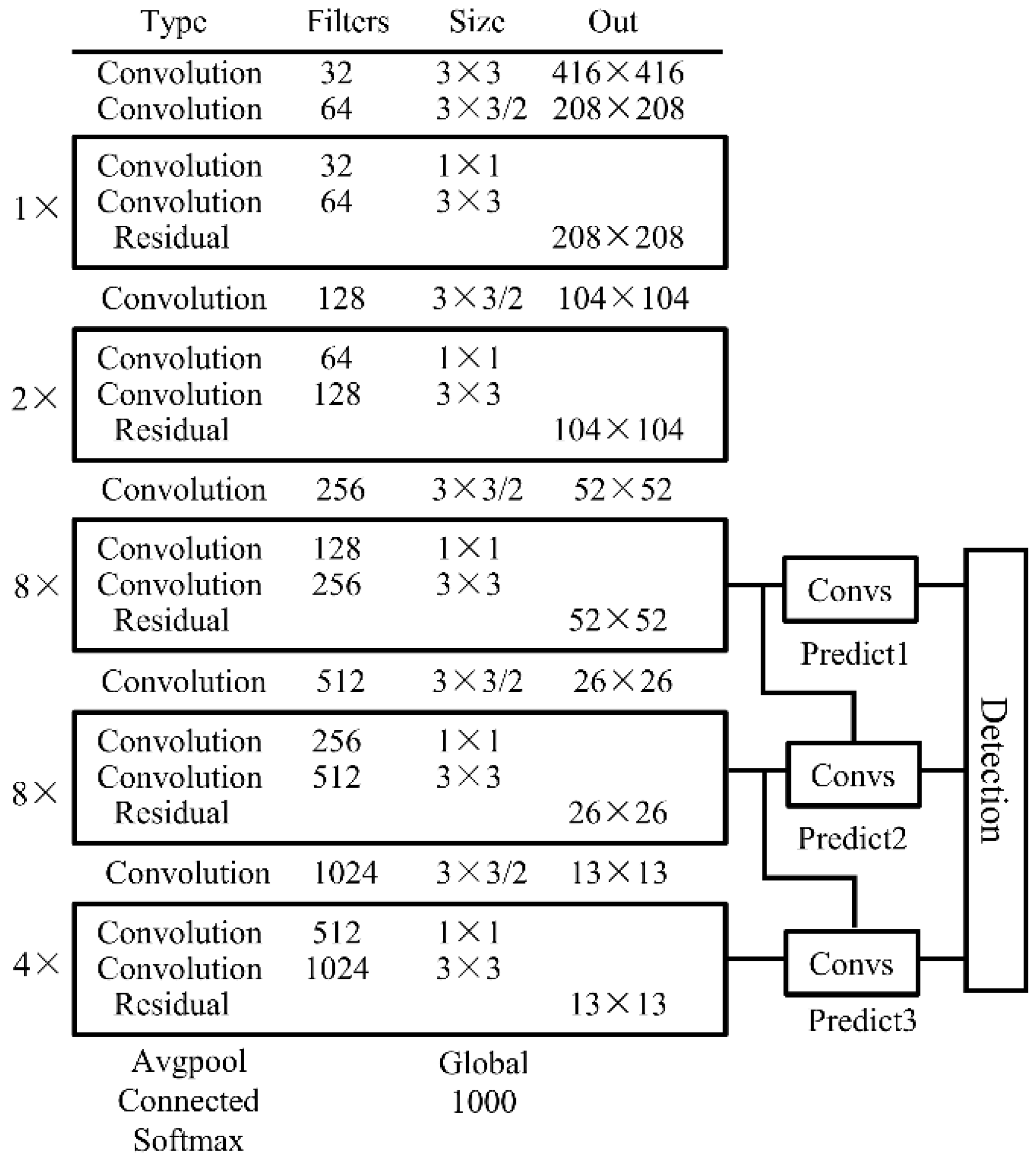
2.2. YOLO-V3 Deep Neural Network

The You Only Look Once, Version 3/YOLO-V3 [33] algorithm is an improved algorithm based on YOLO and YOLO-V2. In contrast to two-stage target detection algorithms, such as Faster R-CNN, it divides the image into different grids. Each grid is responsible for the corresponding object, and supports multi-category target detection. Faster detection speeds can be achieved while maintaining accuracy. Additionally, YOLO-V3 can achieve its average precision with a higher detection speed than a one-stage network [34,35].

There are two main components to the YOLO-V3 detection model: a backbone network and a detection network. Its network structure is shown in Figure 3. The algorithm uses several excellent 3 × 3 and 1 × 1 convolution kernels, and some residual structures are used in the later multi-scale predictions. Figure 3 shows the adoption of Darknet-53, based on the residual network idea, as the backbone network for feature extraction. As part of the training process of the network layer deepening model, the Darknet-53 model consisted of five residual blocks to prevent gradient explosions. Each residual block consisted of multiple residual units, which contained two DBL units. The DBL units each contained a convolution layer (Con2d Layer), a batch normalization layer (BN Layer), and a leaky rectified linear layer (LeakyReLU Layer). In this way, the number of layers in the network could be significantly increased while avoiding the disappearance of gradients.

The detection network part adopted the FPN feature pyramid structure used in the Faster R-CNN to reduce feature loss as much as possible and improve detection accuracy. Among them, a total of 3 feature layers were extracted: the middle layer with the output feature resolution of 52 × 52, the middle and lower layers of 26 × 26, and the bottom layer of 13 × 13. The three feature layers passed the detection for small, medium, and large resolution target objects, respectively. After obtaining 3 effective feature layers, multi-feature fusion was performed, and the effective feature layers were predicted. As soon as the prediction result was obtained, the decoding prediction module decoded the data processed by the network, thereby obtaining the final result.

2.3. Object Tracking Algorithms

Object tracking, locating an object in successive frames of a video, is a core research scheme of computer vision and image processing technology. As for the commonly used object tracking algorithms in OpenCV Python, Kernelized Correlation Filters/KCF tracker uses a combination of BOOSTING and MIL tracking algorithm techniques, and both the accuracy and speed are improved. The Discriminative Correlation Filter with Channel and Spatial Reliability/CSRT tracker is an advanced algorithm with a higher accuracy and lower speed than the KCF tracker. In this study, after conducting multiple trials with different models, the CSRT Tracker model was adopted to track objects.

2.4. Computer Hardware Parameters

The computer hardware parameters of the training platform were as follows: Intel Core i7-4790 @ 3.60 GHz CPU, 32 GB DDR4 RAM, NVIDIA GTX GeForce 2060 GPU with 11 GB memory, and the Windows 10 operating system.

3. Experiments

3.1. Experimental Description

The on-site measurement of curling stone motion was performed at the “Ice Cube” rink designed for the 2022 Beijing Winter Olympics. Information about the investigated curling ice rink and the measuring method are briefly presented in this section.

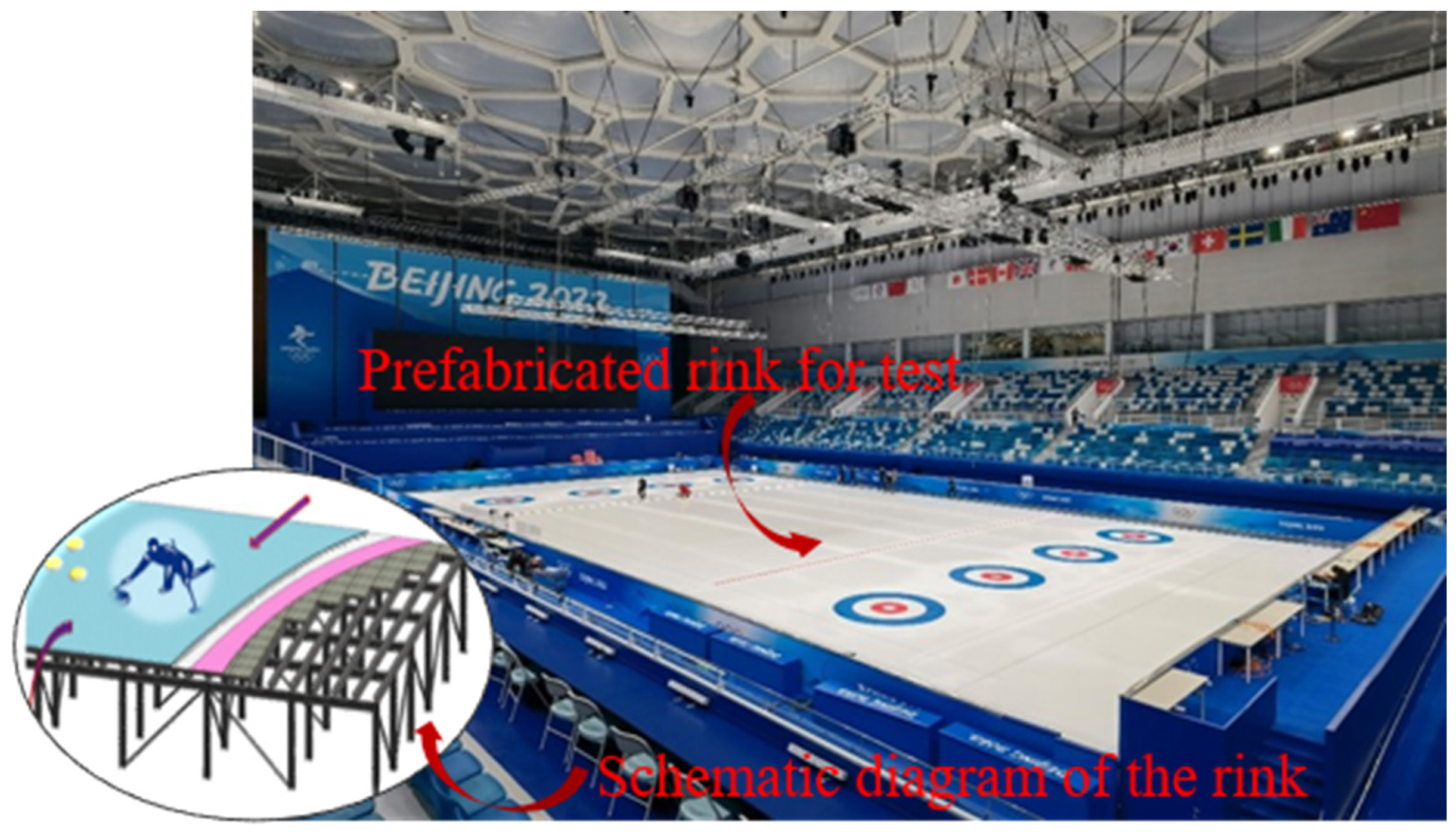
3.1.1. Curling Ice Rink for Beijing Winter Olympics

The prefabricated ice rink, located in the Notational Aquatics Center, in Beijing, China, as shown in Figure 4, was constructed to host the curling event in the 2022 Beijing Winter Olympics. In contrast to traditional ice rinks built directly on rigid concrete bases, the prefabricated rink was built on a swimming pool, using a steel frame and concrete slab supporting system. The ice sheet was 80 mm thick, into which a network of cooling pipes and honeycomb web elements were embedded [36,37]. The thickness of the ice sheet in a traditional curling rink is about 50 mm. The pebbled ice was carefully prepared by the ice-making technician, and the ice surface temperature was maintained at −5 °C. The temperature and humidity ratios of the air closest to the ice sheet and the air 1500 mm above the ice sheet were 7~9 °C/2~3 g/kg and 12~14 °C/3~3.5 g/kg, respectively.

3.1.2. Methods of Measurements

A high-precision camera with a resolution of 3840 × 2160 pixels attached at 2000 mm above the ice surface was adopted to record the curling stone motion at 60 frames/s. As pointed out by the previous surveyed literature, the stone rotation and sweeping of the pebbled ice generate transverse motion. For simplicity, in the present study, video recording of the movement of the stones was performed without rotation and sweeping. The comprehensive stone motion, combined with rotation and sweeping, will be carried out in future studies. The sliding distance of the stone recorded in each test was about 3 m, due to the limitation of the camera monitoring the area. A total of 100 groups of experiments with different initial velocities were conducted.

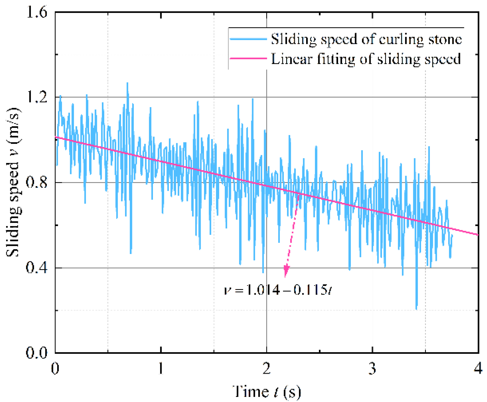
3.2. Data Processing

As shown in Figure 5, the stone–ice friction coefficient was obtained by performing the following processing flow on the recorded video data. The CSRT tracker algorithm was used to track curling stone motion, and the pixel coordinates of the marked points were obtained frame-by-frame. Before calculating the acceleration in real coordinates, the pixel coordinates were required to be converted into real ones. The coordinate transformation coefficient k was obtained according to the relationship between the actual distance determined by the ruler placed on the ice surface and the distance between pixel points. Therefore, determination of the real displacements, speeds, and accelerations of the curling stone was archived. Using the actual position coordinates, the average speed in a small timestep, as an approximate value of instantaneous speed, was calculated by substituting the formula $v=\Delta x/\Delta t$.

Figure 6 shows the relationship between the sliding speed of a curling stone and the corresponding time during a throwing motion. Linear fitting of the sliding speed was performed, and the slope of the straight line was related to the deceleration produced by friction force. Finally, the corresponding friction coefficient of a stone sliding on an ice surface was calculated according to the formula $\mu =a/g$, where g is the gravitational acceleration. For an example given in Figure 6, a deceleration of 0.115 m/s² can be obtained, and the stone–ice friction coefficient would be calculated as 0.0117.

During the above-mentioned data processing approach, the change in friction coefficient a was ignored, i.e., the sliding speed linearly decreased with time. Furthermore, it seemed reasonable to adopt a constant friction coefficient within a short sliding distance of less than 3 m. Assuming a stone sliding at an initial speed of v₀ with a constant acceleration a, the displacement–time relationship would be described as $y={\nu }_{0}t+\frac{1}{2}a{t}^2$, where y is the displacement of the stone and t is the time interval. Figure 7 shows the stone-sliding distance versus time curve and the fitting results using the linear function and quadratic function, respectively. It can be observed that the quadratic function corresponding to a uniformly decreased motion showed good agreement with the measured data, when compared with the linear equation corresponding to a uniform motion. According to the result of fitting the sliding distance with a quadratic function, the friction coefficient was taken as 0.0116, which was consistent with the above obtained value of 0.0117.

4. Results and Discussion

In this section, the results of the measured friction coefficient using deep-learning-based methods are presented. The velocity-dependent stone–ice friction coefficient was described using a mixed lubrication regime. Moreover, the friction coefficient obtained from on-site measurement in this study was compared with that of other curling rinks (the predicted values were compared by different theoretical models), and the experimental results were based on another measurement method, using an accelerometer sensor.

4.1. Impact of Velocity on Friction Coefficient

Statistical methods were adopted to present our experimental results. The speed range was divided into 14 groups (0.35~0.45 m/s, 0.45 m/s~0.55 m/s,…, 1.35 m/s~1.45 m/s), and the average value and corresponding standard deviation of the friction coefficient in each interval were calculated. Figure 8 presents the influence of the average sliding velocity on the friction coefficient between the ice and curling stone. It can be seen that the curling stone on the ice had a low coefficient of friction, ranging from 0.006 to 0.016. Similarly to other ice friction conditions, such as ice–ice friction [38], the low values of stone–ice friction were attributed to the presence of a thin lubricating water film on the ice surface. With regard to the velocity-dependent friction strength, results from the measurements showed descending coefficient of friction values as the curling stone sliding velocity increased, and different forms of functions were used to describe the trend of decreasing friction strength (Figure 8). However, the fitting results were poor because of the scatter of the friction coefficient values, which could have been attributed to the uncertainty of the complex contact conditions between the stone RB and pebbled ice. Another reason could have been related to the measurement method, i.e., the friction coefficient was determined based on the change in sliding speed, instead of the required force to maintain a constant speed of the stone.

According to the thickness of the liquid-like layer, three different friction regimes are typically distinguished: dry friction, mixed friction, and hydrodynamic friction. In the mixed friction regime, the thickness of the liquid-like layer is lower than the characteristic roughness, and the friction coefficient decreases with the thickness of the liquid-like layer, which is formed with increasing temperature, pressure, or sliding velocity. Therefore, the phenomenon of higher velocity resulting in a more pronounced effect on the reduction in the friction indicated that more lubricating water film was formed with the increasing sliding speed, due to frictional heating and the stone–ice friction belonging to a mixed lubrication regime.

As presented in Figure 9, publicly available friction data of curling stones based on experimental measurements were collected to compare with our obtained values. It can be noted that the friction coefficient in our work was mainly measured at speeds of 0.5 m/s to 1.4 m/s, whereas the literature data was usually obtained at speeds of less than 0.5 m/s. Regarding the speed dependency of the friction, it can be observed that the literature data agreed with our measured results. However, as stone–ice friction is a very complex tribological system, the differences in the absolute values could have been related to different experimental parameters, such as the ice rink, ice surface temperature, surface roughness, air temperature, and humidity.

Table 1. Experimental parameters of stone–ice friction coefficients.

Reference	Curling Rink	Ice Surface Temperature	Air Temperature and Relative Humidity	Sliding Velocity
Penner [19]	Nanaimo curling rink in Canada	−5 °C	Not available	0.15~1 m/s
Nyberg et al. [20]	Curling ice prepared by Daniel Svensson at Curlingcompaniet	−3.5 °C	6~7 °C and 55%	0.1~2.3 m/s
This study	Prefabricated curling rink for Winter Olympics	−5 °C	7~9 °C and ~39%	0.4~1.4 m/s

summarizes some available experimental parameters for the measurement of the stone–ice friction coefficient.

4.2. Assessment of the Theoretical Models for Stone–Ice Friction

In this section, the performance of the two published theoretical models mentioned in the introduction for calculating stone–ice friction coefficients is discussed, based on the data we obtained.

In the process of theoretical derivation by Penner [19], the complex contact conditions between the stone and pebbled ice were simplified as n points with square contact areas. According to the relationship between the energy produced by friction force and the energy transferred into the ice, the coefficient of kinetic friction was obtained with the following equation:

$$\mu =\frac{1}{\sqrt{2}}{\left(k_i{\rho }_i{c}_i\right)}^{\frac{1}{2}}{n}^{\frac{1}{4}}{p}^{-\frac{3}{4}}{F}_n{}^{-\frac{1}{4}}\Delta T{\nu }^{-\frac{1}{2}}$$

(1)

where k_i, ρ_i, and c_i are the thermal conductivity, density, and specific heat capacity, respectively, of the ice; n is the contact point between the stone and ice; p is the interface pressure, according to the assumption made by Makkonen and Tikanmaki [39] and Lozowski et al. [40], i.e., the ice hardness multiplied by the actual contact area is equal to the exerted load, giving an ice hardness of 35 MPa; F_n is the total normal force between the stone and ice; ∆T is the temperature difference between the ice surface temperature and the bulk ice temperature; and v is the stone sliding velocity.

Lozowski et al. [26] derived a friction coefficient function based on thermodynamic equilibrium, without considering the details of dry and wet friction. On the basis of an assumption that the total friction force exerted on the curling stone is composed of shear stress force and the ploughing force, the numerical model of the stone–ice friction coefficient was calculated as follows:

$$\mu =\frac{2}{H\nu }\left[\frac{k_g\Delta T_g}{\sqrt{\pi {\kappa }_g{t}_p}}+\frac{k_i\Delta T_i}{\sqrt{\pi {\kappa }_i{t}_b}}\right]$$

(2)

with

$$\begin{array}{l}\Delta T_g=T_{melt}-T_g\\ \Delta T_i=T_{melt}-T_i\\ t_p=\frac{2r_p}{\nu }\\ t_b\in [t_b^{\min },t_b^{\max }]\\ t_b^{\min }=\frac{b}{\nu }\\ t_b^{\max }=\frac{2\sqrt{2rb+b^2}}{\nu }\end{array}$$

where H is the ice hardness (35 MPa); T_i, T_g, and T_melt are ice surface temperature, curling stone RB temperature and melting point temperature of the ice, respectively; t_b is the contact time between the curling stone RB and a point on the pebble; t_p is the contact time between the pebble and a point on the curling stone RB; r_p is the radius of the top contact of a pebble (1.5 mm); v is the stone sliding speed; b is the width of the curling stone RB (6 mm); r is the inner radius of the curling stone RB (60 mm); k_g and k_i are the thermal conductivities of the ice (2.3 Wm⁻²K⁻¹) and the Blue Hone granite (2.94 Wm⁻²K⁻¹), respectively; and ${\kappa }_i$ and ${\kappa }_g$ are the thermal diffusivities of the ice (1.23 × 10⁻⁶ m²s⁻¹) and the Blue Hone granite (1.49 × 10⁻⁶ m²s⁻¹), respectively.

Figure 10 presents the obtained results from on-site measurement and the values calculated from the Penner model and the Lozowski model. It can be seen that most of the experimental results in this study were within the range of the upper and lower limits predicted by the Lozowski model. In terms of the two theoretical models, as shown in Equations (1) and (2), both of the predicted friction coefficient values were related to the sliding speed in the form of $\mu \propto {\nu }^{-\frac{1}{2}}$. Therefore, the curve shapes of the friction coefficients versus the speed of the two models seemed to be consistent with each other. However, it can be found that the calculated values by the Penner model were lower than the Lozowski model under the same ice parameters, such as hardness and thermal conductivity. In fact, the heat generated by friction in the Penner model was only considered to be conducted into the ice, while the heat transferred to the stone and melted ice was ignored. Hence, the energy dissipated by friction was calculated lower than the actual value, resulting in a decrease in the friction coefficient.

4.3. Verification of the Measured Values Using Accelerometer-Based Method

In recent years, sensor technology has been increasingly used in sports engineering to acquire various sport information [41,42,43,44]. To verify the friction results obtained using computer vision technology, a sensor-based measurement method was also adopted to measure the stone–ice friction. An accelerometer weighing 30 g was attached to the curling stone, using an epoxy resin adhesive. The measurement range and voltage sensitivity of the accelerometer were ±5 g and 1002 mV/g, respectively. The acceleration signal of the curling stone in the sliding direction was collected at a sampling frequency of 50 Hz by the TEST data acquisition system. As in the previous case, the stone was released without initial rotation velocity to avoid the curling phenomenon.

Figure 11 shows the collected time–history curve of the acceleration of the curling stone, thrown on a standard pebbled ice sheet. A slight fluctuation of the raw signal during stone motion was observed, and the friction coefficient was obtained by averaging the raw data. This averaging approach has been used to obtain steel–ice friction coefficients by a tribometer [24,45]. According to the average acceleration data presented in Figure 12, the friction coefficient of a stone sliding on ice with an average speed of ~0.85 m/s was obtained as 0.014 ± 0.003 using the formula $\mu =a/g$, where a is the measured acceleration and g is the gravitational acceleration.

Figure 12 presents the friction coefficient values using an accelerometer-based method. The results obtained by the method based on the accelerometer sensor were generally consistent with those obtained by our proposed procedure based on the YOLO-V3 deep neural network. Therefore, the method based on deep learning was effective and reliable, and could be further used to monitor the change in friction coefficient for curling competitions in real time.

5. Limitation and Future Work

The purpose of this study was to investigate the stone–ice friction coefficient in a prefabricated ice rink for the 2022 Beijing Winter Olympics, using a deep-learning-based method. This study had the following limitations, which need to be further studied in the future:

(1)

Only a curling stone with a linear motion trajectory was considered. The transverse motion component caused by stone rotation and ice sweeping was neglected, which is most common in ice rinks. Further studies on the friction mechanism of a curling stone following a curled trajectory are needed.

(2)

In this prefabricated rink for the 2022 Beijing Winter Olympics, a surface topography analysis of the pebbled ice was not conducted, due to the limitations of the experiment equipment. Further research is needed to study the influence of the surface topography characteristics of pebbled ice on the stone–ice friction coefficient to reach a more nuanced conclusion.

(3)

It should be noted that the friction coefficient obtained in this research is not applicable for the description of friction strength under ice-sweeping circumstances. During the ice-sweeping process, the thickness of the liquid-like layer is increased, which was ascribed to the ice temperature increasing by frictional heating and the melting point of the ice decreasing by considerable pressure. In fact, the thickness of the liquid-like layer on the ice surface has a great influence on the friction strength.

6. Conclusions

In this paper, an experimental investigation on the coefficient of friction between a curling stone and pebbled ice was conducted at the “Ice Cube” rink, using a computer vision technology method. The displacement, velocity, and acceleration of sliding stones were extracted frame-by-frame from video data using our proposed procedure based on the YOLO-V3 deep neural network and CSRT Object tracking algorithm. The effect of the sliding velocity on the stone–ice friction coefficient was discussed, and comparisons of our obtained results with other research reported values were performed. In addition, assessment of the theoretical models for stone–ice friction and verification of the obtained results through a sensor-based method were conducted. With respect to experimental results and discussion, some of the following conclusions could be drawn:

• The proposed measurement method based on computer vision technology could be used to obtain the friction coefficient of a curling stone and ice, and the obtained results were in accordance with the law of stone–ice friction, and in good agreement with the related literature data. The computer vision technology based on deep learning can be further employed to monitor the ice quality of the curling rink in real time.
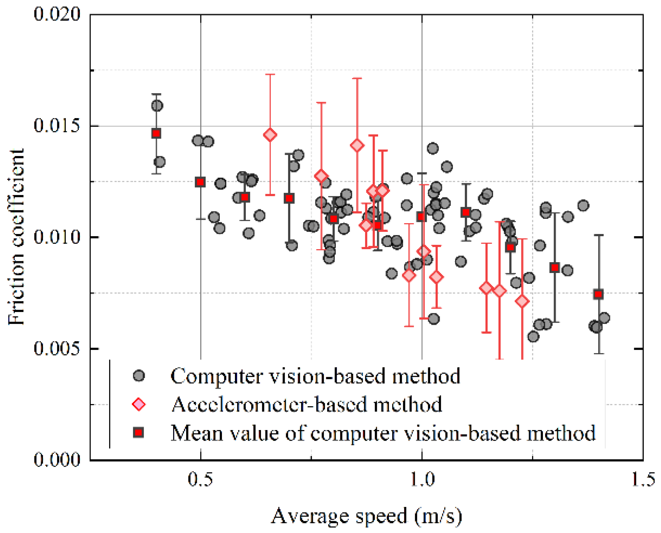
• The coefficient of friction between a curling stone and ice, ranging from 0.006 to 0.016, was significantly affected by the stone sliding speed. Increasing the curling stone sliding speed resulted in lower friction coefficient values, due to the formation of a lubricating water film generated by the friction heat.
• The Lozowski model had a better performance in describing the relationship between the speed and friction. Most of our experimental results were included within the upper and lower limits predicted by the Lozowski model. Under the same ice parameters, the predicted value of the Penner model was lower than that of the Lozowski model, because it ignored the heat generated by friction transferred to the stone and melted ice.
• The accelerometer-based method was additionally employed to measure the stone–ice friction coefficient. The good agreement between the obtained values of our proposed procedure based on the YOLO-V3 deep neural network and that of the accelerometer sensor supported the effectiveness and reliability of the deep-learning-based method.

References

1. Kim, T.W.; Lee, S.C.; Kil, S.K.; Choi, S.H.; Song, Y.G. A Case Study on Curling Stone and Sweeping Effect According to Sweeping Conditions. Int. J. Environ. Res. Public Health 2021, 18, 833. [Google Scholar] [CrossRef]
2. Gwon, J.; Kim, H.; Bae, H.; Lee, S. Path Planning of a Sweeping Robot Based on Path Estimation of a Curling Stone Using Sensor Fusion. Electron 2020, 9, 457. [Google Scholar] [CrossRef] [Green Version]
3. Maeno, N. Dynamics and Curl Ratio of a Curling Stone. Sport. Eng. 2014, 17, 33–41. [Google Scholar] [CrossRef] [Green Version]
4. Zhang, W.; Li, J.; Yang, Q.; Mu, L. Practical Application of a Novel Prefabricated Curling Ice Rink Supported by Steel–Concrete Composite Floors: In Situ Measurements of Static and Dynamic Response. Structures 2021, 32, 1888–1906. [Google Scholar] [CrossRef]
5. Maeno, N. Assignments and Progress of Curling Stone Dynamics. Proc. Inst. Mech. Eng. Part P J. Sport. Eng. Technol. 2016, 494–497. [Google Scholar] [CrossRef]
6. Bradley, J.L. The Sports Science of Curling: A Practical Review. J. Sport. Sci. Med. 2009, 8, 495–500. [Google Scholar]
7. Denny, M. Curling Rock Dynamics: Towards a Realistic Model. Can. J. Phys. 2002, 80, 1005–1014. [Google Scholar] [CrossRef]
8. Jensen, E.T.; Shegelski, M.R.A. The Motion of Curling Rocks: Experimental Investigation and Semi-Phenomenological Description. Can. J. Phys. 2004, 82, 791–809. [Google Scholar] [CrossRef]
9. Nyberg, H.; Hogmark, S.; Jacobson, S. Calculated Trajectories of Curling Stones Sliding under Asymmetrical Friction: Validation of Published Models. Tribol. Lett. 2013, 50, 379–385. [Google Scholar] [CrossRef]
10. Kameda, T.; Shikano, D.; Harada, Y.; Yanagi, S.; Sado, K. The Importance of the Surface Roughness and Running Band Area on the Bottom of a Stone for the Curling Phenomenon. Sci. Rep. 2020, 10, 20637. [Google Scholar] [CrossRef]
11. Maeno, N. Curl Mechanism of a Curling Stone on Ice Pebbles. Bull. Glaciol. Res. 2010, 28, 1–6. [Google Scholar] [CrossRef]
12. Shegelski, M.R.A.; Lozowski, E. First Principles Pivot-Slide Model of the Motion of a Curling Rock: Qualitative and Quantitative Predictions. Cold Reg. Sci. Technol. 2018, 146, 182–186. [Google Scholar] [CrossRef]
13. Shegelski, M.R.A.; Lozowski, E. Pivot-Slide Model of the Motion of a Curling Rock. Can. J. Phys. 2016, 94, 1305–1309. [Google Scholar] [CrossRef]
14. Ziegler, M. The Split Friction Model-The Isotropic Origin of the Lateral Force in Curling. Res. Sq. 2022, 1–14. [Google Scholar] [CrossRef]
15. Hattori, K.; Tokumoto, M.; Kashiwazaki, K.; Maeno, N. High-Precision Measurements of Curling Stone Dynamics: Curl Distance by Digital Image Analysis. Proc. Inst. Mech. Eng. Part P J. Sport. Eng. Technol. 2016, 1754337116679061. [Google Scholar] [CrossRef]
16. Denny, M. A First-Principles Model of Curling Stone Dynamics. Tribol. Lett. 2022, 70, 84. [Google Scholar] [CrossRef]
17. Denny, M. Ice Deformation Explains Curling Stone Trajectories. Tribol. Lett. 2022, 70, 41. [Google Scholar] [CrossRef]
18. Braghin, F.; Cheli, F.; Melzi, S.; Sabbioni, E.; Maldifassi, S. The Engineering Approach to Winter Sports; The Engineering Approach to Winter Sports; Springer: Berlin/Heidelberg, Germany, 2016; ISBN 9781493930203. [Google Scholar]
19. Penner, A.R. The Physics of Sliding Cylinders and Curling Rocks. Am. J. Phys. 2001, 69, 332. [Google Scholar] [CrossRef] [Green Version]
20. Nyberg, H.; Alfredson, S.; Hogmark, S.; Jacobson, S. The Asymmetrical Friction Mechanism That Puts the Curl in the Curling Stone. Wear 2013, 301, 583–589. [Google Scholar] [CrossRef]
21. Makkonen, L.; Tikanmäki, M. Modeling the Friction of Ice. Cold Reg. Sci. Technol. 2014, 102, 84–93. [Google Scholar] [CrossRef]
22. Kietzig, A.M.; Hatzikiriakos, S.G.; Englezos, P. Physics of Ice Friction. J. Appl. Phys. 2010, 107, 4. [Google Scholar] [CrossRef]
23. Spagni, A.; Berardo, A.; Marchetto, D.; Gualtieri, E.; Pugno, N.M.; Valeri, S. Friction of Rough Surfaces on Ice: Experiments and Modeling. Wear 2016, 368, 258–266. [Google Scholar] [CrossRef]
24. Scherge, M.; Böttcher, R.; Spagni, A.; Marchetto, D. High-Speed Measurements of Steel-Ice Friction: Experiment vs. Calculation. Lubricants 2018, 6, 26. [Google Scholar] [CrossRef] [Green Version]
25. The Kinetic Friction of Ice. Proc. R. Soc. London A Math. Phys. Sci. 1976, 347, 493–512. [CrossRef]
26. Lozowski, E.P.; Szilder, K.; Maw, S.; Morris, A.; Poirier, L.; Kleiner, B. Towards a First Principles Model of Curling Ice Friction and Curling Stone Dynamics. In Proceedings of the International Offshore and Polar Engineering Conference, Kona, HI, USA, 21–26 June 2015. [Google Scholar]
27. Marian, M.; Tremmel, S. Current Trends and Applications of Machine Learning in Tribology—A Review. Lubricants 2021, 9, 86. [Google Scholar] [CrossRef]
28. Rosenkranz, A.; Marian, M.; Profito, F.J.; Aragon, N.; Shah, R. The Use of Artificial Intelligence in Tribology—A Perspective. Lubricants 2021, 9, 2. [Google Scholar] [CrossRef]
29. Zhang, Q.; Zhang, B.; Chen, C.; Li, L.; Wang, X.; Jiang, B.; Zheng, T. A Test Method for Finding Early Dynamic Fracture of Rock:Using DIC and YOLOv5. Sensors 2022, 22, 6320. [Google Scholar] [CrossRef]
30. Teng, S.; Liu, Z.; Li, X. Improved YOLOv3-Based Bridge Surface Defect Detection by Combining High- and Low-Resolution Feature Images. Buildings 2022, 12, 1225. [Google Scholar] [CrossRef]
31. Wang, D.; Liu, Z.; Gu, X.; Wu, W.; Chen, Y. Automatic Detection of Pothole Distress in Asphalt Pavement Using Improved Convolutional Neural Networks. Remote Sens. 2022, 14, 3892. [Google Scholar] [CrossRef]
32. Redmon, J.; Divvala, S.; Girshick, R.; Farhadi, A. You Only Look Once: Unified, Real-Time Object Detection. In Proceedings of the IEEE Computer Society Conference on Computer Vision and Pattern Recognition, Las Vegas, NV, USA, 26 June–1 July 2016. [Google Scholar]
33. Redmon, J.; Farhadi, A. YOLOv3: An Incremental Improvement. arXiv 2018, arXiv:1804.02767. [Google Scholar]
34. Li, Y.; Zhang, X.; Shen, Z. YOLO-Submarine Cable: An Improved YOLO-V3 Network for Object Detection on Submarine Cable Images. J. Mar. Sci. Eng. 2022, 10, 1143. [Google Scholar] [CrossRef]
35. Kou, X.; Liu, S.; Cheng, K.; Qian, Y. Development of a YOLO-V3-Based Model for Detecting Defects on Steel Strip Surface. Meas. J. Int. Meas. Confed. 2021, 182, 109454. [Google Scholar] [CrossRef]
36. Zhang, W.; Li, J.; Wang, L.; Yuan, B.; Yang, Q. Flexural Characteristics of Artificial Ice in Winter Sports Rinks: Experimental Study and Nondestructive Prediction Based on Surface Hardness Method. Arch. Civ. Mech. Eng. 2022, 22, 1–9. [Google Scholar] [CrossRef]
37. Zhang, W.; Li, J.; Yuan, B.; Wang, L.; Yang, Q. Experimental Investigation of Unconfined Compressive Properties of Artificial Ice as a Green Building Material for Rinks. Buildings 2021, 11, 586. [Google Scholar] [CrossRef]
38. Wang, Q.; Li, Z.; Lu, P.; Cao, X.; Leppäranta, M. In Situ Experimental Study of the Friction of Sea Ice and Steel on Sea Ice. Appl. Sci. 2018, 8, 675. [Google Scholar] [CrossRef] [Green Version]
39. Serré, N. Numerical Modelling of Ice Ridge Keel Action on Subsea Structures. Cold Reg. Sci. Technol. 2011, 67, 107–119. [Google Scholar] [CrossRef]
40. Lozowski, E.; Szilder, K.; Maw, S. A Model of Ice Friction for a Speed Skate Blade. Sport. Eng. 2013, 16, 239–253. [Google Scholar] [CrossRef]
41. Dzikowski, B.; Weremczuk, J.; Pachwicewicz, M. Acceleration-Based Method of Ice Quality Assessment in the Sport of Curling. Sensors 2022, 22, 1074. [Google Scholar] [CrossRef]
42. Dzikowski, B.; Pachwicewicz, M.; Weremczuk, J. Inertial Measurements of Curling Stone Movement. In Proceedings of the 2018 15th International Scientific Conference on Optoelectronic and Electronic Sensors, COE, Warsaw, Poland, 17–20 June 2018. [Google Scholar]
43. Lozowski, E.; Maw, S.; Kleiner, B.; Szilder, K.; Shegelski, M.; Musilek, P.; Ferguson, D. Comparison of IMU Measurements of Curling Stone Dynamics with a Numerical Model. In Proceedings of the Procedia Engineering, Budapest, Hungary, 4–7 September 2016. [Google Scholar]
44. van der Kruk, E.; den Braver, O.; Schwab, A.L.; van der Helm, F.C.T.; Veeger, H.E.J. Wireless Instrumented Klapskates for Long-Track Speed Skating. Sport. Eng. 2016, 19, 273–281. [Google Scholar] [CrossRef] [Green Version]
45. Ovaska, M.; Tuononen, A.J. Multiscale Imaging of Wear Tracks in Ice Skate Friction. Tribol. Int. 2018, 21, 280–286. [Google Scholar] [CrossRef]
Figure 1. Contact situation of curling stone and pebbled ice.
Lubricants 10 00265 g001
Figure 2. Apparatus for friction force measurement of sliding stone on ice. Adapted from [18].
Lubricants 10 00265 g002
Figure 3. Model structure of YOLO-V3 (You Only Look Once, Version 3) deep neural network.
Lubricants 10 00265 g003
Figure 4. The prefabricated curling rink for 2022 Beijing Winter Olympics.
Lubricants 10 00265 g004
Figure 5. Flowchart for calculating the coefficient of friction from raw data.
Lubricants 10 00265 g005
Figure 6. Example of the sliding speed of curling stone obtained during movement.
Lubricants 10 00265 g006
Figure 7. Example of the sliding distance of curling stone during movement.
Lubricants 10 00265 g007
Figure 8. Relationship between friction coefficient and average sliding speed: (a) Measured data; (b) Average value and standard deviation.
Lubricants 10 00265 g008
Figure 9. Comparison of stone–ice friction coefficients [19,20].
Lubricants 10 00265 g009
Figure 10. Friction coefficient predicted by numerical models [19,26].
Lubricants 10 00265 g010
Figure 11. Acceleration signal collected by accelerometer during sliding of curling stone.
Lubricants 10 00265 g011
Figure 12. Friction coefficient results obtained by an accelerometer sensor.
Lubricants 10 00265 g012