Observer-Based Control of Tilting-Pad Thrust Bearings


Abstract
:1. Introduction
2. Observer Design
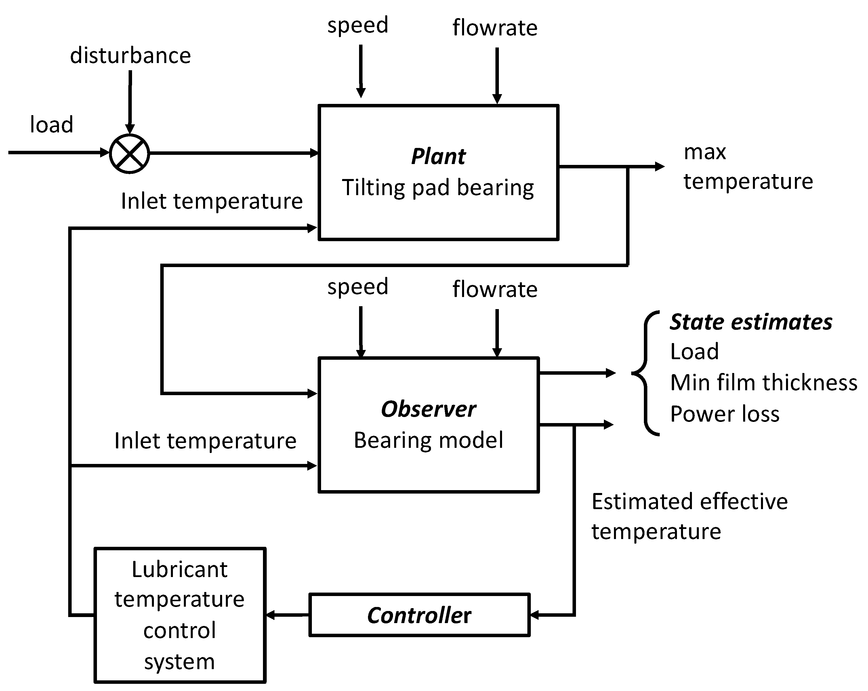
2.1. Observer Design Based on ESDU 83004
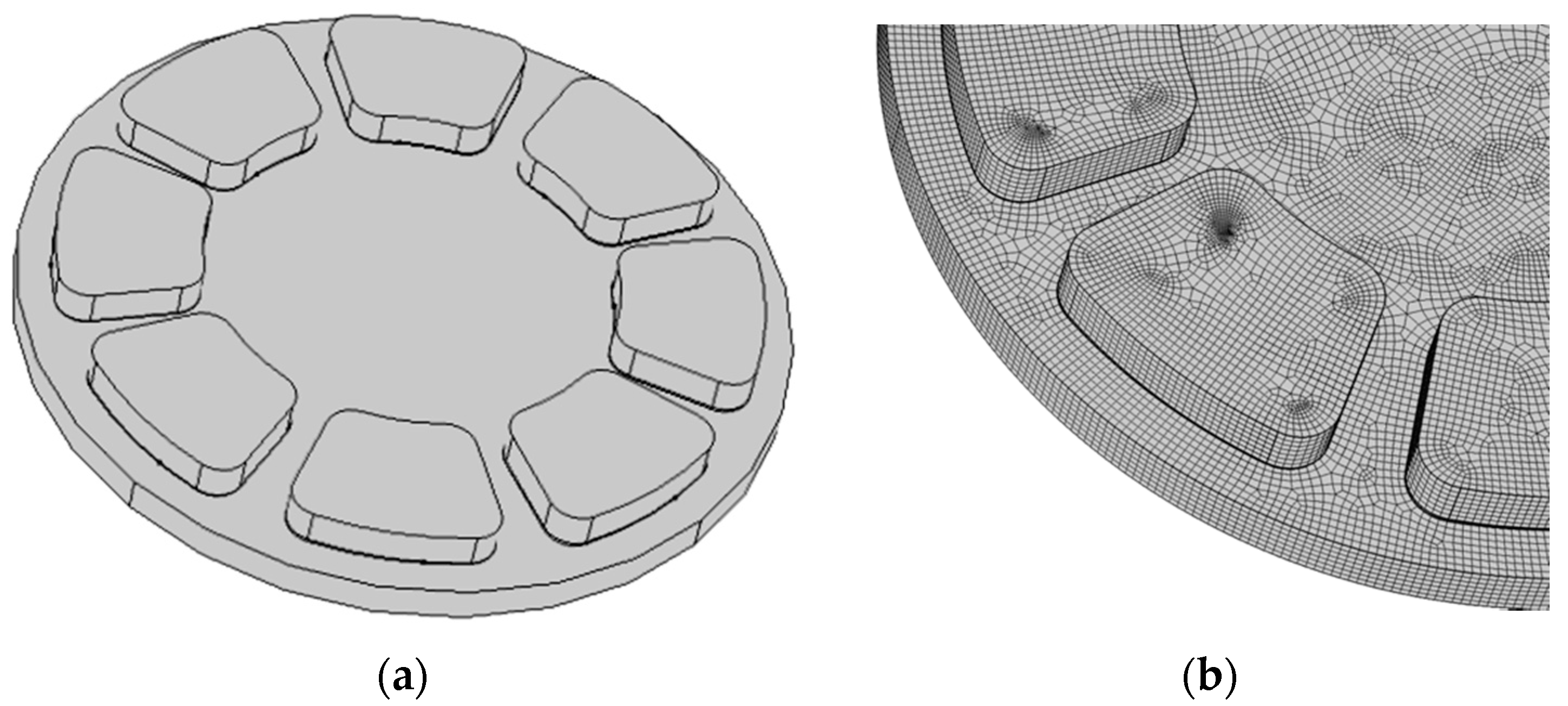
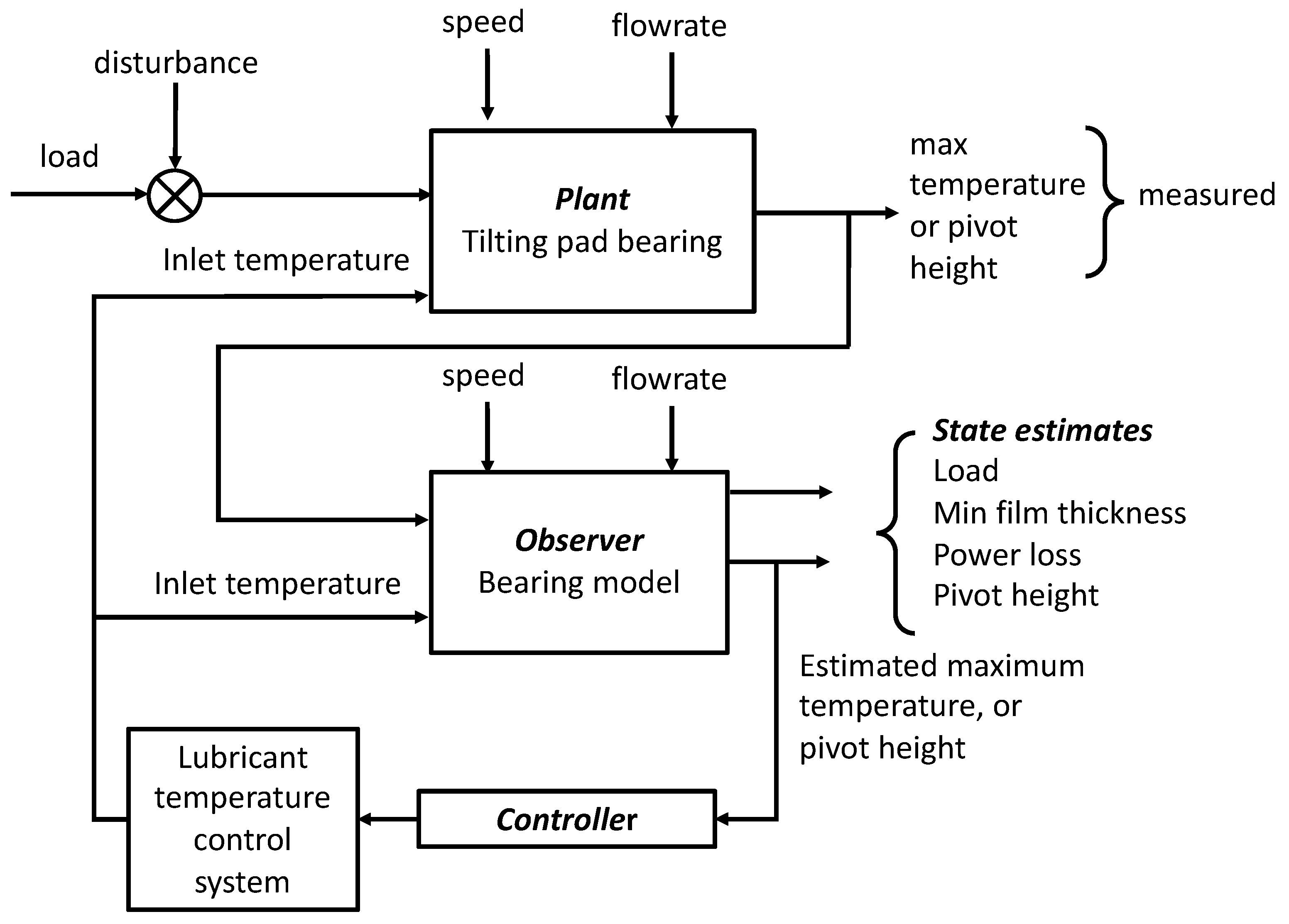
2.2. Observer Design Based on FE Modelling
3. Running the Observers
3.1. The ESDU-Based System
| Load | 2739 N |
| Power loss per pad | 547 W |
| Load | 3424 N (+25%) |
| (−15%) | |
| Power loss per pad | 583 W (+7%) |
| Load | 3424 N |
| Power loss per pad | 525 W |
3.2. The FE-Based System
| a pivot height of 49.2 | (a decrease of 18%) |
| a min. film thickness of 20.0 | (a decrease of 20%) |
| an effective temperature of 56.6 °C | (an increase of 3%) |
| an applied load of 4881 N | (an increase of 72%) |
| power loss of 218 W | (an increase of 22%) |
| a min. film thickness of 24.1 μm | (a decrease of 4.4%) |
| a maximum temperature of 69.0 °C | (an increase of 0.7%) |
| an effective temperature of 55.8 °C | (an increase of 0.3%) |
| an applied load of 3787 N | (an increase of 4.9%) |
| a power loss of 198 W | (an increase of 0.4%) |
4. Conclusions
Funding
Institutional Review Board Statement
Informed Consent Statement
Conflicts of Interest
Disclaimer
Appendix A
Appendix B

| Inlet Temperature Tin (degC) | Pivot Height hp (μm) | Tilt (rad) | Force per Pad, w (N), | Mean Viscosity, | Max_pad_temp, Tmax (°C) | Minimum Film Thickness hmin (μm) | Mean Fluid Temp, Te (°C) | Power Loss per Pad z (W) |
|---|---|---|---|---|---|---|---|---|
| 50 | 40 | 0.0012240 | 6226.5 | 0.078142 | 75.19 | 15.948 | 59.134 | 228.5 |
| 50 | 50 | 0.0015175 | 4679.8 | 0.089024 | 71.562 | 20.18 | 56.495 | 214.72 |
| 50 | 60 | 0.0017955 | 3585.1 | 0.096495 | 68.593 | 24.718 | 54.869 | 199.05 |
| 50 | 70 | 0.0020635 | 2806 | 0.10178 | 66.107 | 29.451 | 53.793 | 183.79 |
| 50 | 80 | 0.0023210 | 2246.5 | 0.10583 | 64.014 | 34.391 | 53.008 | 170.05 |
| 60 | 40 | 0.0011610 | 4284.7 | 0.05216 | 78.43 | 17.186 | 66.371 | 162.35 |
| 60 | 50 | 0.0014460 | 3081.5 | 0.057505 | 74.984 | 21.585 | 64.308 | 145.83 |
| 60 | 60 | 0.0017180 | 2297.8 | 0.061058 | 72.41 | 26.241 | 63.101 | 131.27 |
| 60 | 70 | 0.0019810 | 1763.5 | 0.063473 | 70.426 | 31.072 | 62.34 | 118.53 |
| 60 | 80 | 0.0022410 | 1390.4 | 0.065169 | 68.884 | 35.963 | 61.831 | 107.6 |
| 70 | 40 | 0.0011060 | 3070.6 | 0.036353 | 83.94 | 18.267 | 74.583 | 120.18 |
| 70 | 50 | 0.0013700 | 2075.5 | 0.038194 | 80.64 | 23.079 | 72.907 | 101.74 |
| 70 | 60 | 0.0016380 | 1492.5 | 0.039374 | 78.394 | 27.813 | 72.002 | 87.978 |
| 70 | 70 | 0.0019030 | 1121.7 | 0.040156 | 76.806 | 32.605 | 71.462 | 77.347 |
| 70 | 80 | 0.0021650 | 871.44 | 0.040695 | 75.643 | 37.457 | 71.113 | 68.895 |
| 80 | 40 | 0.0010990 | 2428.3 | 0.028603 | 90.811 | 18.404 | 83.485 | 95.223 |
| 80 | 50 | 0.0013620 | 1625.2 | 0.029739 | 88.199 | 23.236 | 82.181 | 80.052 |
| 80 | 60 | 0.0016220 | 1155 | 0.03037 | 86.4 | 28.127 | 81.479 | 68.599 |
References
- Ulbrich, H.; Althaus, J. Actuator Design for Rotor Control. In Proceedings of the 12th Biennial Conference on Vibration and Noise, Montreal, QC, Canada, 17–21 September 1989; pp. 17–22. [Google Scholar]
- Santos, I.F. Design and Evaluation of Two Types of Active Tilting Pad Journal Bearings. In Active Control of Vibration; Burrows, C.R., Keogh, P.S., Eds.; Mech. Eng. Publication Ltd.: London, UK, 1994; pp. 79–87. [Google Scholar]
- Deckler, D.C.; Veillette, R.J.; Cho, F.K.; Braun, M.J. Modelling of a Controllable Tilting Pad Bearing. In Proceedings of the American Control Conference, Albuquerque, NM, USA, 4–6 June 1997. [Google Scholar]
- Deckler, D.C.; Veillette, R.J.; Braun, M.J.; Cho, F.K. Simulation and Control of an Active Tilting-Pad Journal Bearing. Tribol. Trans. 2004, 47, 440–458. [Google Scholar] [CrossRef]
- Vivaros, H.P.; Nicoletti, R. Lateral Vibration Attenuation of Shafts Supported by Tilting-Pad Journal Bearing With Embedded Electromagnetic Actuators. J. Eng. Gas Turbines Power 2014, 136, 042503. [Google Scholar] [CrossRef]
- Wu, M.F.; Cavalva, K.L. Experimental validation and comparison between different active control methods applied to a journal bearing supported rotor. Struct. Control. Health Monit. 2019, 26, e2446. [Google Scholar] [CrossRef]
- Morosi, S.; Santos, I.F. Experimental Investigations of Active Air Bearings. In Proceedings of the ASME Turbo Expo 2012: Turbine Technical Conference and Exposition. Volume 7: Structures and Dynamics, Parts A and B, Copenhagen, Denmark, 11–15 June 2012; ASME. pp. 901–910. [Google Scholar] [CrossRef]
- Babin, A.; Kornaev, A.; Rodichev, A.; Savin, L. Active thrust fluid-film bearings: Theoretical and experimental studies. Proc. Inst. Mech. Eng. Part J J. Eng. Tribol. 2020, 234, 261–273. [Google Scholar] [CrossRef]
- Santos, I.F. Trends in Controllable Oil Film Bearings. In IUTAM Symposium on Emerging Trends in Rotor Dynamics; Gupta, K., Ed.; IUTAM Bookseries; Springer: Dordrecht, The Netherlands, 2011; Volume 1011. [Google Scholar] [CrossRef]
- Sanadgol, D.; Maslen, E. Effects of actuator dynamics in active control of surge with magnetic thrust bearing actuation. In Proceedings of the 2005 IEEE/ASME International Conference on Advanced Intelligent Mechatronics, Monterey, CA, USA, 24–28 July 2005; pp. 1091–1096. [Google Scholar] [CrossRef]
- Riaz, M.T.; Rehman, W.U.; Ali, H.; Husnain, S.; Jiang, G.; Lodhi, E.; Aaqib, S.M.; Qureshi, M.M. Design and Experimental Validation of a Small-Scale Prototype Active Aerostatic Thrust Bearing. In Proceedings of the 2021 International Conference on Computing, Electronic and Electrical Engineering (ICE Cube), Quetta, Pakistan, 26–27 October 2021; pp. 1–6. [Google Scholar] [CrossRef]
- Luenberger, D. An Introduction to Observers. IEEE Trans Autom. Control. 1971, 16, 596–602. [Google Scholar] [CrossRef]
- Smith, E.H.; Gill, K.F. Controlling the attitude and two flexure-modes of a flexible satellite. Aeronaut. J. 1977, 81, 41–44. [Google Scholar] [CrossRef]
- Banghu, B.; Bingham, C. Nonlinear state-observer techniques for sensorless control of automotive PMSM’s, including load-torque estimation and saliency. In Proceedings of the European Power Electronics and Drives Conference EPE 2003, Toulouse, France, 2–4 September 2003. [Google Scholar] [CrossRef]
- Eissa, M.A.; Sali, A.; Hassan, M.K.; Bassiuny, A.M.; Darwish, R.R. Observer-Based Fault Detection With Fuzzy Variable Gains and Its Application to Industrial Servo System. IEEE Access 2020, 8, 131224–131238. [Google Scholar] [CrossRef]
- Chen, X.; Su, C.-Y.; Fukuda, T. A nonlinear disturbance observer for multivariable systems and its application to magnetic bearing systems. IEEE Trans. Control. Syst. Technol. 2004, 12, 569–577. [Google Scholar] [CrossRef]
- Rehman, W.U.; Guiyun, J.; Yuan Xin, L.; Yongqin, W.; Iqbal, N.; UrRehman, S.; Bibi, S. Linear extended state observer-based control of active lubrication for active hydrostatic journal bearing by monitoring bearing clearance. Ind. Lubr. Tribol. 2019, 71, 869–884. [Google Scholar] [CrossRef]
- Calculation Methods for Steadily Loaded, Off-Set Pivot, Tilting-Pad Thrust Bearings. ESDU 83004. 1983. pub. IHS EDSDU. Available online: https://www.esdu.com/cgi-bin/ps.pl?sess=unlicensed_1220115034725fdk&t=doc&p=esdu_83004 (accessed on 25 November 2021).
- Comsol Multiphysics, Version 5; COMSOL, Inc.: Avenue Burlington, MA, USA. Available online: https://cn.comsol.com/ (accessed on 25 November 2021).
- Almqvist, T.; Glavatskikh, S.B.; Larsson, R. (June 22, 1999) THD Analysis of Tilting Pad Thrust Bearings—Comparison Between Theory and Experiments. ASME J. Tribol. 2000, 122, 412–417. [Google Scholar] [CrossRef]
| Parameter | Value |
|---|---|
| Load per pad, w | 2750 kN |
| Shaft diameter | 76 mm |
| Rotational speed | 100 rev s−1 |
| Inlet temperature, Tin | 50 °C |
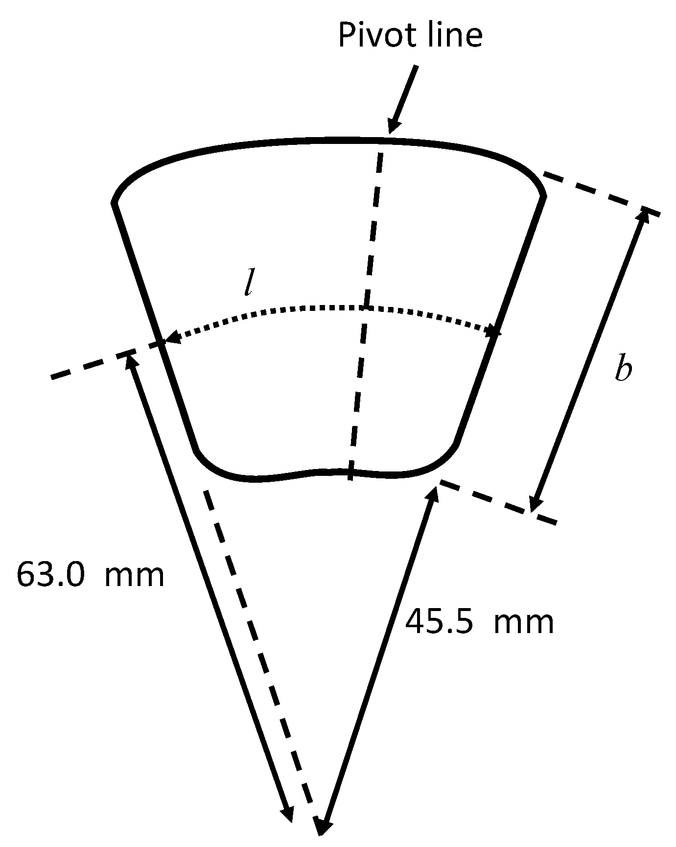
| Pad width, b | 37 mm |
| Pad length, l | 37 mm |
| Inner diameter of pads | 89 mm |
| Mean surface speed, U | 39.6 ms−1 |
| Viscosity at 50 °C | 0.013 Pa-s |
| Viscosity at 100 °C | 0.0036 Pa-s |
| Location of line pivot | 62.5% from leading edge |
| Minimum acceptable film thickness | 15 μm |
| Parameter | Value |
|---|---|
| No of pads | 8 |
| Load per pad, w | 3585 N |
| Inlet temperature, Tin | 50 °C |
| Pad width, b | 40.1 mm |
| Pad length, l | 48.7 mm |
| Inner diameter of pads, dm | 115 mm |
| Mean surface speed, U | 8.12 ms−1 |
| Viscosity at 50 °C | 0.124 Pa-s |
| Viscosity at 100 °C | 0.017 Pa-s |
| Location of line pivot | 65% from leading edge |
| Minimum acceptable film thickness | 15 μm |
| Parameter | Observer estimates | Actual conditions | Error |
|---|---|---|---|
| pivot height | 0.5% | ||
| minimum film thickness | 1.2% | ||
| effective temperature | 55.7 °C | 54.9 °C | 1.5% |
| applied load/ pad | 3609 N | 3585 N | 0.7% |
| power loss/ pad | 194.4 | 199.1 | 2.3% |
| Parameter | Observer estimates | Actual conditions | Error |
|---|---|---|---|
| min. film thickness | 2.0% | ||
| maximum temperature | 68.5 °C | 68.6 °C | 0.1% |
| effective temperature | 55.6 °C | 54.9 °C | 1.3% |
| applied load/pad | 3574 N | 3585 N | 0.3% |
| power loss/pad | 193.7 | 199.1 | 2.7% |
Publisher’s Note: MDPI stays neutral with regard to jurisdictional claims in published maps and institutional affiliations. |
© 2022 by the author. Licensee MDPI, Basel, Switzerland. This article is an open access article distributed under the terms and conditions of the Creative Commons Attribution (CC BY) license (https://creativecommons.org/licenses/by/4.0/).
Share and Cite
Smith, E.H. Observer-Based Control of Tilting-Pad Thrust Bearings. Lubricants 2022, 10, 11. https://doi.org/10.3390/lubricants10010011
Smith EH. Observer-Based Control of Tilting-Pad Thrust Bearings. Lubricants. 2022; 10(1):11. https://doi.org/10.3390/lubricants10010011
Chicago/Turabian StyleSmith, Edward H. 2022. "Observer-Based Control of Tilting-Pad Thrust Bearings" Lubricants 10, no. 1: 11. https://doi.org/10.3390/lubricants10010011
APA StyleSmith, E. H. (2022). Observer-Based Control of Tilting-Pad Thrust Bearings. Lubricants, 10(1), 11. https://doi.org/10.3390/lubricants10010011