Abstract
I outline the history of and progress in observing and understanding quasar multi-frequency and multi-messenger variability from the point of view of someone who has been working in the field for over 30 years. I will present some important references for the evolution from optical monitoring to multi-frequency cooperative programs that revealed the true multi-frequency/multi-timescale nature of variability in these objects. Quasar observations began with separate radio and optical monitoring programs; then the optical and radio observations w ere combined. This was followed by expanding the analyses to include far IR, UV, X-rays, and finally adding gamma rays. This progression yielded simultaneous multi-frequency spectra of these objects and light curves over 15 decades in frequency. The future is adding particle (neutrino) and gravitational waves to the picture. I also present long-term (50 years) optical light curves, and discuss optical variability at all timescales from minutes to tens of years in some selected objects for which we have reliable long-term monitoring observations.
1. Introduction
My introduction to quasars began as an undergraduate physics major interested in astronomy. I began by reading Ben Bova’s book “In Quest of Quasars” [1], followed by a book entitled “Quasi-Stellar Objects” [2] by Geoffrey and Margaret Burbidge. The term quasar is short for Quasi-Stellar Radio Sources. The term “Blazar” is used to describe quasars characterized by rapid high amplitude variations on short timescales and exhibit high polarization. Blazars are divided into subclasses of BL Lac objects and OVV or flat spectrum quasars. The BL Lac objects have spectra similar to BL Lacertae’s spectrum in that they are devoid of broad emission lines. Blazars are thought to be oriented such that we are essentially looking down the jet axis of a quasar. When Alex Smith from the University of Florida visited Ball State and gave a talk about his work with quasars I become interested his work and knew I wanted to study with him. I graduated with a Bachelor’s degree in physics and minor in astronomy (1981), applied and was accepted for graduate school at the University of Florida and began observing quasars as part of Dr. Smith’s NSF supported research program using the technology of the time to monitor quasar optical variability: Photographic photometry. I was using the 30-inch telescope at Rosemary Hill observatory (RHO) equipped with hyper-sensitized photographic plates sensitive to Johnson V, B, and PG filter systems. The telescope had a clock drive but required guiding for the duration of the 6 or 10-min exposures. Guiding was done by staring into a small guide scope and using a hand-paddle for real-time manual input of tracking corrections as the guide star drifted from the cross hairs in the guide scope. During the exposures, the observer was perched at the top of a ladder at the Newtonian focus of the 30-inch telescope. The photographic technology utilized cutting-edge hyper-sensitizing chemical technology (baking Kodak plates in hydrogen and other chemicals to increase sensitivity) [3]. The plates were exposed through the appropriate filter window in air-tight cassettes in an atmosphere of dry nitrogen to protect them from the harmful effects of moisture from the Florida environment. They were immediately developed in the observatory darkroom and examined to determine the magnitude of the source using Arglander’s method (comparing the image to calibration stars by eye) to see if the quasar was in outburst. The plates were taken back to the lab and measured using a Cuffy iris photometer [4] to get accurate magnitudes. The Iris photometry technology routinely yielded magnitudes with accuracies of +/−0.1 magnitude. Data collected in this manner showed that not only were there several magnitudes of variability over long periods of time, but also optical outbursts of several magnitudes over days and weeks [5,6]. Table 1 lists a sample of the sources and number of monitoring observations made at the RHO funded by the NSF under the supervision of Alex Smith.

Table 1.
Sample of RHO most observed objects.
It was during one evening at the telescope when I was trying to identify the field of my next target PKS 1156+295, but I could not match the stars I was seeing in the telescope eyepiece with the finder chart printed on the index card finding charts! The Blazar was in outburst and so bright it was visible through the eyepiece which is why I could not identify the field. That outburst was a key piece in the upcoming multi-frequency observations (1981) [7]. Many other multi-frequency papers followed utilizing our optical observations, the radio monitoring observations from the University of Michigan [8] combined with observations by the International Ultraviolet Explorer telescope (IUE) [9,10,11,12]. Our group at the University of Florida then began studying the optical variability of X-ray selected quasars [13]. I received grant funding from NASA ADS to go through the EINSTEIN X-ray observatory archive and reduce X-ray observations of a sample of our quasars. This culminated in my Master thesis studying the effect that significant optical variations had on X-ray-optical correlations and the diffuse X-ray background [14]. I learned that unless optical variability was included in these studies, the resulting correlations would not be useful in accounting for the X-ray background. I analyzed ESOSAT X-ray observations of quasars to search for periodic signals or to characterize the types of noise embedded in the signals. No periodicities or anything other than random noise was detected in the EXOSAT light curves of our sources [15].
My colleague Ian McHardy and I analyzed simultaneous X-ray and optical observations of an outburst in PKS 1156+295 [16]. For my PhD thesis, I studied the simultaneous multi-frequency variability of a sample of quasars over the E-M spectrum including Michigan radio data, IRAS IR, RHO optical, IUE and EINSTEIN X-ray observations [17]. Using this data I showed that Synchrotron Self Compton (SSC) + accretion disk models can accurately replicate the observed simultaneous multi-frequency spectrum from X-ray to radio throughout the entire variability range, and yielding reasonable parameter fits by adjusting only two parameters (electron normalization and accretion rate).
After graduate school, I accepted a visiting professor position at Stephen F. Austin State University (1988) and I turned my attention to studying the individual outbursts in interesting sources and testing gravitational lens explanations for quasar variability [18]. I also considered periodic variations in the long-term light curves using time series analysis [19]. OJ 287 is another object I have studied intensively, and it has been modeled as a binary black hole system by [20]. The binary black hole model postulates a central massive black hole and a secondary black hole which orbits the primary. As the secondary black hole smashes through the accretion disk of the primary black hole one would expect optical outbursts. This would imply predictable outbursts sequences. The binary black hole model has continued to evolve and is still a possible model to explain the long-term variations and major outbursts seen in this violently variable active source.
I accepted a position at the Goddard Space flight Center in Greenbelt Maryland as resident astronomer and scheduler for the International Ultraviolet Explorer (IUE) satellite ultraviolet spectrograph (1989). IUE was capable of observing the spectra of quasars. While I had to run shifts for other observers, I managed to get a chunk of observing time for myself and began coordinating my observing runs on IUE with RHO observers and others around the world. Other IUE Observers like Joel Bregman and Megan Urry had been doing IUE observations of quasars for a number of years, so I joined them in continuing the multi-frequency observations with IUE using my own observing time to drive observing programs [21,22,23].
I then accepted a tenure track faculty position at Florida International University in Miami Florida (1991). I was determined to find a way to continue to monitor quasars and contribute to variability studies of Blazars. Terry Oswalt was instrumental in establishing the Southeastern Association for Research in Astronomy (SARA) consortium. SARA was a group of five universities who had submitted a proposal to the NSF and won the #1 0.9-m de-commissioned telescope at Kitt Peak National Observatory. SARA decided to rebuild the telescope as a remotely accessible observatory at Kitt Peak. Florida International University joined as a new member in the SARA consortium and we built a new dome and hired Astronomical consultants and Equipment (ACE) to automate it, and it has been in operation ever since [24]. Since the first observations from the Kitt Peak telescope in 1990, the SARA consortium has added two more research telescopes to its stable. The acquisition of the Lowell 24” telescope at Cerro Tololo and the JKT 1-m at Roque de los Muchochos observatories gave the SARA members additional observing possibilities. I continued to monitor quasars using the SARA telescopes, but narrowed my observing list to OVV Blazars.
While visiting the Goddard Space flight center in Greenbelt in 1993, I met with the EGRET team associated with the new Compton Gamma-Ray Observatory who had seen my recent papers on 3C 279 and 3C 345 [25,26]. I worked with the EGRET team that summer compiling multi-frequency observations from various groups around the world contemporaneous with the gamma-ray detections. This work resulted in the nearly simultaneous multi-wavelength spectrum and variability of 3C 279 from 109 to 1024 Hz for the first time. This was followed-up by more observations [27,28].
In 2013, I raised money and designed $2.4 million dollar Stocker AstroScience Center [29] on the MMC campus of Florida International University (FIU). The primary telescope at the Stocker AstroScience Center is a 24” ACE reflector telescope complete with research grade CCD and UBVRI filters. I have continued monitoring my list of Blazars using the SARA telescopes and the Stocker telescope and concentrated on studying the rapid intraday or micro-variability of a few very active objects. I also continued to participate and contribute to international multi-frequency collaborations including the Whole Earth Blazar Telescope Consortium (WEBT) campaigns [30,31,32], and serving as principle investigator on one project which obtained a 72-h micro-variability of BL Lac object S5 0716+71. This was the first time an extended micro-variability curve was attempted [33]. Lately, satellites such as KEPLER and TESS have provided longer micro-variability curves.
Micro-variability or intraday variability is extremely rapid (hours), low amplitude variations (0.1 magnitudes) seen intermittently in many Blazars. These observations and theoretical interpretations of them continue to evolve and are presented in a companion paper in this volume. In the next section, I present some of these optical observations over timescales ranging from years to days.
2. Materials and Methods
The quasar monitoring program at the University of Florida started in 1969 and ran until 1990. All observations were done with photographic photometry and the group observed 101 objects, mostly in B and PG filter bands though some V filtered images were made. Table 1 is a small sample of the available observations of the most observed quasars. The RHO program was funded by NSF grants until 1988, after which Alex Smith retired and the data was nearly lost. I rescued most of the data after the program ceased to exist in 1990. The recent data not published in the [5,6] papers referenced is currently available upon request.
The actual dates and magnitudes of most of these observations were published in their entirety up until 1988 [5].
I continued to monitor a subset of objects including those listed in Table 1 from 2003 to present. I observed 19 objects concentrating on micro- or intraday variability. In the Table 2, each night might represent 200 individual images since I mostly looked for micro-variability.
Table 2.
SARA-FIU observing list.
I combined the RHO data and the newer CCD observations to produce long-term light curves for several of the objects. The following long-term light curves use historical photographic data back to 1928, the Rosemary Hill photographic data (B-band), and more recent data from the SARA data. The R magnitudes were converted to B using empirically determined offsets for each source. Comparing B observations to R-band observations is also dangerous since the Blazar spectra tend to be power laws that have variable in slope, and when comparing different epochs the transformation may have changed. However, for this analysis we did a least squares fit of the offset for many different nights and different flux levels and found the offset error is not large enough to affect the general conclusions. Some light curves were supplemented with data from Smarts, Tuorla and other monitoring observations from the literature. Proper care must be taken when including observations from other programs. Most importantly the filter CCD combinations yielding a standard calibration and the comparison stars are the same. The best way is comparing calibrated observations taken on the same night and gauging the match in the resulting magnitudes. This was carefully done in this analysis.
3. Results
Figure 1a–h shows the long-term light curves of several well observed Blazars. The data before 1954 were gleaned from the Harvard plate archives by Dr. Joe Pollock and were added to the photographic Florida observations. The data points after 1995 are from my FIU monitoring program, and other observatory archives.
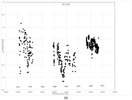
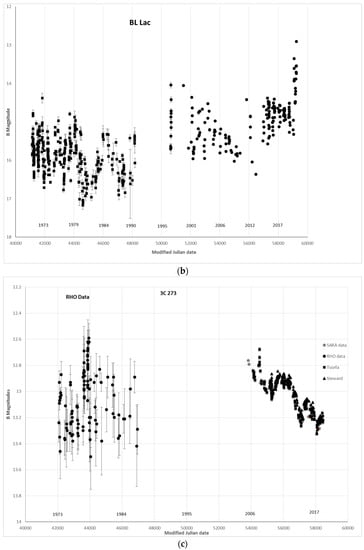
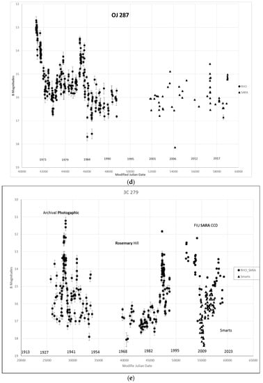
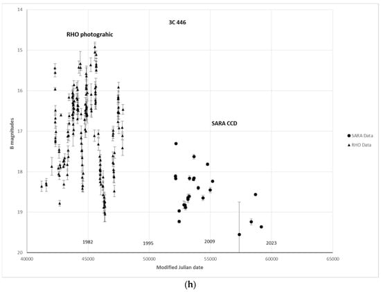
Figure 1.
(a). The long-term light curve of 3C 120. The B band minus R band offset for this source was determined to be mB-mR = 2.0. N = 775 data points are shown in the plot. (b). The long-term light curve of BL Lacertae. The B band minus R band offset for this source was determined to be mB-mR = 1.543 magnitudes; 1623 data points data points are shown in the plot. (c). The long-term light curve of 3C 273. The blue band minus R band offset for this source was determined to be mB-mR = 1.0 magnitudes, N = 91 data points are shown in the plot. (d). The long-term light curve of OJ 287. The blue band minus R band offset for this source was determined to be mB-mR = 1.503, N = 376 data points are shown in the plot. (e). The Long-term light curve of 3C 279. The B band minus R band offset for this source was determined to be mB-mR = 1.0 magnitudes, N = 282 data points are shown in the plot. (f). The long-term light curve of 1156+295. The B band minus R band offset for this source was determined to be mB-mR = 1.0 magnitudes, N = 268 data points are shown in the plot. (g). The long-term light curve of AO 0235+164. The blue band minus R band offset for this source was determined to be mB-mR = 2.0 magnitudes, N = 497 data points are shown in the plot. (h). The long-term light curve of 3C 446. The blue band minus R band offset for this source was determined to be mB-mR = 1.0 magnitudes. N = 174 data points are shown in the plot.
These light curves were analyzed for long-term characteristics such as the variability quantity Q which is defined as the change in brightness dB over the average error: Q = dB/(σavg). We calculated Q for the light curves presented here by dividing the light curve up to segments to see how the variability changes over time. The first segment is the RHO data that is approximately 30 years of photographic observations. The second segment is the SARA and recent CCD observations that are of similar duration of about 30 years. Figure 2 lists the long-term variability behavior of our target objects, Column 1 is the source name, column 2 the redshift, column 3 the Q values for the Historical data (RHO) and the more recent observations. Column 4 lists the average magnitudes of the segments. Upward pointing arrow in the Q column shows an increase in amplitude of variability as time goes on, while an upward pointing arrow in the average magnitude column indicates the objects average magnitude is apparently increasing over time. Large gaps in the light curves between the RHO and recent observations correspond to the cessation of NSF funding for the RHO program. Data from other monitoring programs may fill in some of the gaps.
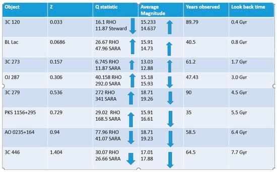
Figure 2.
The long-term variability behavior of 8 Blazars over nearly 100 years of monitoring observations.
Figure 1a depicts the long-term behavior of 3C 120. It does not show violently explosive outbursts like some others, but varies more slowly over time. It appears to be getting slightly brighter over time.
Figure 1b shows the long-term light curve of BL Lac. This is one of the most exciting and active object on our monitoring list. Its average magnitude is noticeably increasing as its activity level. Recent outbursts of several magnitudes in a few weeks have been observed. No periodic variation has been proposed for this object.
Figure 1c is the light curve of 3C 273. While I have never considered 3C 273 very active or exciting to observe, it does vary significantly but the amplitude of variability is only one magnitude.
The long-term light curve of OJ 287 is shown in Figure 1d. While the high amplitude outbursts are not periodic, the outbursts have been modelled as systematic variations of a binary black hole model [20]. The average magnitude appears to be decreasing, and from the data presented in this LC is uncertain how it evolves. However, there are recent publications [34] that show the brightness of this object has increased recently, and the various temporal behaviors (with quasi-periodicities at ~60 years, ~12 years, and ~1 year) appear to be supported by the overall data collected over the last 100 years.”
Figure 1e shows the long-term light curve of the extremely OVV quasar 3C 279. This object has been routinely monitored and displays outbursts in many different frequency bands including gamma rays [27].
Figure 1f is the long-term light curve of PKS 1156+295 that I find the most fascinating of all of these sources. Its brightness is unpredictable and experience three magnitude outbursts in a week. The very definition of an optically violent variable object.
Figure 1g shows AO 0235+164. This object is episodic and exhibits rapid three and four magnitude outbursts that range between 11 and 18th the magnitude. Many observations had upper limits of 19th magnitude yet 0235 was not visible. The average magnitude is slightly fainter in recent observations but not significantly.
4. Discussion
A quick examination of Figure 2 shows there is no apparent correlation between the increase/decrease of brightness levels and the activity levels overall. Some objects increase in brightness level but decrease in activity level (3C 120), while others increase in brightness and activity level (BL Lac (BL) and 3C 273 (OSO)). Other objects decreased in brightness and increased in activity level (OJ 287 (BL), 3C 279(OVV), and PKS 1156+295(OVV)). Two objects (0235+164 (BL) and 3C 446(OVV) decreased both in brightness and activity level. No noticeable trends occur nor does it seem to depend on type of Blazar, (BL Lac vs. OVV quasar).
It has been a pleasure to participate in the expansion of Quasar observations over the entire electromagnetic spectrum. It should be noted that I have referenced many of the studies I worked on, but there were many other groups doing similar work. In fact even the papers I have listed have dozens of co-authors, so this work was not done in a vacuum. Each paper contained experts in a particular region of the E-M spectrum and the results were synthesized. The advance of instruments that allowed this work to happen is also important to note. The availability of satellite telescopes over the E-M spectrum was timely and necessary. In the UV part of the spectrum we progressed from IUE (1978) to ST and GALEX, and finally Swift (2004). Infrared Observatories capable of doing this work began with IRAS (1983) to WISE (2009). The next improvement will be when the JWST to be launched in 2021. In the X-ray part of the spectrum EINSTEIN (1978) was the first instrument capable of making important observations of quasars, Currently NuStar (2012) is making these observations. The gamma ray spectral region began with SAS II (1972), which was followed by CGRO in 1991 and culminated with FERMI (2008). Further contributing to our understanding during this period of time was the evolution of telescopes in each spectral region. Perhaps the most important being the development of VLBI techniques in the radio part of the spectrum that was capable of imaging the inner regions of the Blazar jets. This procedure of achieving high resolution radio images began in the 1960′s and culminated this past year in the EHT image of the black hole in M87 and the innermost jet in 3C 279 with unprecented resolution.
Several important aspects of quasar models have been confirmed using multi-frequency variability observations. Supermassive black holes are most likely at the heart of the quasars. The central black hole is almost certainly fed by an accretion disk. The multi-frequency spectrum and variability observations indicate that the synchrotron-Compton models work better than other models to explain the observed spectrum and variability. Whether it is SSC or synchrotron with External Compton scattering (EC) remains in question. Optical monitoring programs have yielded light curves nearly 100 years in duration. The change in technology has complicated the analysis. With photographic plates we monitored variability primarily in the B band, but CCD imaging is done primarily in the R band because of the sensitivity of the detectors and the fact that relatively small aperture telescopes are used for long-term monitoring. The light curves were plotted with B magnitudes on the y axis. The transformation from R to B was done individually for each object. The years of optical and multi-frequency studies have led to interpretations of the variations over the three major time frames.
- Long-term variability is baseline fluctuations on timescales of years and tens of years. These variations are most likely linked to the fueling the supermassive black holes and interactions with the host galaxies. Figure 2 shows that the variability characteristics change with time, but not in consistent fashion. Some objects have brightened over time while others are fainter, and the variability range is sometimes larger and sometimes smaller.
- Short-term outbursts, weeks to months, seem to be related to shock waves propagating in the relativistic jets stimulated by accretion events. [35] Amplitudes of several magnitudes in a week are common among many different objects.
- Extremely short-term variability, micro-variations that seem to be related to turbulence in the jet flow [36].
I look forward to the future of adding gravitational waves (LISA) and neutrinos (TX 0537) [37] to the total picture so we can get an even more complete picture of the phenomena which holds clues to galaxy formation and the evolution of the universe. The detection of neutrinos from Blazars is particularly exciting since we are now looking at nuclear processes that are undoubtedly occurring but not represented in the E-M spectrum view. We will have to wait a while to detect gravitational waves but it will be worth the wait.
Funding
This research received no external funding.
Data Availability Statement
Data used in these graphs can be requested from the author.
Acknowledgments
The author would like to acknowledge the comments and input form the anonymous referees who made the manuscript much better. He would also like to acknowledge all of those who worked with him throughout the 30-year journey. “The Remote Observatories of the Southeastern Association for Research in Astronomy (SARA)” by W. Keel et al. (2017, PASP, 129, 015002). The authors are honored to be permitted to conduct astronomical research on Iolkam Du’ag (Kitt Peak), a mountain with particular significance to the Tohono O’odham Nation. Bonning et al. (2012), mentioned above, and with the following: “This paper has made use of up-to-date SMARTS optical/near-infrared light curves that are available at www.astro.yale.edu/smarts/glast/home.php (accessed on 24 August 2021)”.
Conflicts of Interest
The authors declare no conflict of interest.
References
- Bova, B. In Quest of Quasars; Signet: New York, NY, USA, 1975; ISBN 10 0451614119. [Google Scholar]
- Quasi-Stellar Objects—Geoffry and Margaret Burbidge. W.H. Freeman and Co. Publishers: New York, NY, USA, 1967; ISBN 10 0716703211.
- Scott, R.L.; Smith, A.G.; Webb, J.R. Hypersensitizing the Kodak IV-N Emulsion. AAS Photo-Bull. 1985, 40, 5. [Google Scholar]
- Cuffy, J. Tests of an improved Iris Photometer. Astron. J. 1955, 60, 157. [Google Scholar] [CrossRef]
- Pica, A.J.; Webb, J.R.; Smith, A.G.; Bitran, M. Long-Term Optical Behavior of 144 Compact Extragalactic Objects: 1969–1988. Astron. J. 1988, 96, 1215. [Google Scholar] [CrossRef]
- Webb, J.R.; Smith, A.G.; Leacock, R.J.; Fitzgibbons, G.L.; Gombola, P.P.; Shepherd, D.W. Optical Variations of 22 Violently Variable Extragalactic Sources: 1968–1986. Astron. J. 1988, 95, 374. [Google Scholar] [CrossRef]
- Wills, B.J.; Pollock, J.T.; Aller, H.D.; Aller, M.F.; Balonek, T.J.; Barvainis, R.E.; Binzel, R.P.; Chaffee, F.H.; Dent, W.A.; Douglas, J.N.; et al. The QSO 1156+295: A Multifrequency Study of Recent Activity. Astrophys. J. 1982, 274, 62–85. [Google Scholar] [CrossRef]
- UMRAO Database Interface. Available online: https://dept.astro.lsa.umich.edu/datasets/umrao.php (accessed on 10 October 2020).
- Bregman, J.N.; Glassgold, A.E.; Huggins, P.J.; Neugebauer, G.; Soifer, B.T.; Matthews, K.; Elais, J.; Webb, J.R.; Pollock, J.T.; Pica, A.J.; et al. Multifrequency Observations of the Superluminal Quasar 3C 345. Astrophys. J. 1986, 301, 708–726. [Google Scholar] [CrossRef][Green Version]
- Brown, L.M.J.; Robson, E.I.; Gear, W.K.; Crosthwaite, R.P.; McHardy, I.M.; Hanson, C.G.; Geldzahler, B.J.; Webb, J.R. The Spectral Shape and Variability of the Blazar 3C 446. Mon. Not. R. Astron. Soc. 1986, 219, 671–686. [Google Scholar] [CrossRef][Green Version]
- Bregman, J.N.; Glassgold, A.E.; Huggins, P.J.; Kinney, A.L.; McHardy, I.; Webb, J.R.; Pollock, J.T.; Leacock, R.J.; Smith, A.G.; Pica, A.J.; et al. Multifrequency Observations of the Optically Violent Variable Quasar 3C 446. Astrophys. J. 1987, 331, 1987. [Google Scholar] [CrossRef]
- Bregman, J.N.; Glassgold, A.E.; Huggins, P.J.; Neugebauer, G.; Soifer, B.T.; Matthews, K.; Elias, J.; Webb, J.R.; Pollock, J.T.; Leacock, R.J.; et al. Multifrequency Observations of BL Lacertae. Astrophys. J. 1990, 352, 574. [Google Scholar] [CrossRef][Green Version]
- Pica, A.J.; Webb, J.R.; Smith, A.G.; Leacock, R.J.; Bitran, M. Optical Variability of X-ray Selected QSOs. Astron. J. 1987, 94, 289. [Google Scholar] [CrossRef]
- Webb, J.R. Effects of Optical Variability on X-ray-Optical Correlations. Master’s Thesis, University of Florida, Gainesville, FL, USA, 1985. [Google Scholar]
- Garcia, L.; Webb, J.R.; Gerstman, B.; Nair, A.D. Time Series Analysis of 10 EXOSAT Observations of PKS 2155-30. Bull. Am. Astron. Soc. 1991, 23, 4. [Google Scholar]
- Webb, J.R.; McHardy, I.M. Simultaneous X-ray-Optical Flare in 1156+295. In Proceedings of the Workshop on the Continuum emission of Active Galactic Nuclei, Tucson, AZ, USA, 11–14 January 1986. [Google Scholar]
- 17. Webb. J.R. Analysis of Nearly Simultaneous X-Ray and Optical Observations of Active Galactic Nuclei. Ph.D. Dissertation, University of Florida, Gainesville, FL, USA, 1988.
- Webb, J.R.; Smith, A.G. Observations of the 1987 Outburst of AO 0235+164. Astron. Astrophys. 1989, 220, 65. [Google Scholar]
- Webb, J.R.; Carini, M.T.; Clements, S.; Fajardo, S.; Gombola, P.P.; Leacock, R.J.; Sadun, A.C.; Smith, A.G. The 1987–1990 Optical Outburst of the OVV Quasar 3C 279. Astron. J. 1990, 100, 1452. [Google Scholar] [CrossRef]
- Sillanpaa, A.; Haarla, S.; Valtonen, M.J.; Sundelius, B.; Byrd, G.G. OJ 287: Binary Pair of Supermassive Black Holes. Astrophys. J. 1988, 325, 628. [Google Scholar] [CrossRef]
- Kawai, N.; Matsuoka, M.; Bregman, J.N.; Soifer, B.T.; Balonek, T.J.; Webb, J.R.; Moriarty-Schieven, G.H.; Chambers, K.C.; Hughes, V.A.; Clegg, R.E.S.; et al. Multifrequency Observations of BL Lacertae in 1988. Astrophys. J. 1991, 382, 508. [Google Scholar] [CrossRef][Green Version]
- Webb, J.R. The Nature of the Optical Variations of Seyfert Galaxy 3C 120. Astron. J. 1990, 99, 49. [Google Scholar] [CrossRef]
- Edelson, R.A.; Saken, J.; Pike, G.; Urry, C.M.; George, I.M.; Warwick, R.S.; Miller, H.R.; Carini, M.T.; Webb, J.R. Rapid Ultraviolet Variability in the BL Lacertae Object PKS 2155-30. Astrophys. J. 1991, 372, L9. [Google Scholar] [CrossRef]
- Keel, W.C.; Oswalt, T.; Mack, P.; Henson, G.; Hilwig, T.; Batcheldor, D.; Berrington, R.; De Pree, C.; Hartmnn, D.; Leake, M.; et al. The Remote Observatories of the Southeastern Association for Research in Astronomy (SARA). Publ. Astron. Soc. Pac. 2017, 129, 015002. [Google Scholar] [CrossRef]
- Shrader, C.R.; Webb, J.R.; Balonek, T.J.; Brotherton, M.S.; Wills, B.J.; Wills, D.; Godlin, S.D.; Smith, A.G.; McCollum, B. Optical and Ultraviolet Observations of 3C 279 During Outburst. Astron. J. 1994, 107, 904–909. [Google Scholar] [CrossRef]
- Webb, J.R.; Shrader, C.R.; Balonek, T.J.; Crenshaw, D.M.; Clements, S.; Smith, A.G.; Nair, A.D.; Leacock, R.J.; Gombola, P.P.; Sadun, A.; et al. The Multifrequency Spectral Evolution of Blazar 3C 345 During the 1991 Outburst. Astrophys. J. 1994, 422, 570–585. [Google Scholar] [CrossRef]
- Hartmann, R.C.; Webb, J.R.; Marscher, A.P.; Travis, J.P.; Dermer, C.D.; Aller, H.D.; Aller, M.F.; Balonek, T.J.; Bennett, K.; Bloom, S.D.; et al. Simultaneous Multiwavelength Spectrum and Variability of 3C 279 from 109 to 1024 Hz. Astrophys. J. 1996, 461, 698. [Google Scholar]
- Wehrle, A.E.; Pian, E.; Urry, M.; Maraschi, L.; McHardy, I.M.; Lawson, A.J.; Ghisellini, G.; Hartman, R.C.; Madejski, G.M.; Makino, F.; et al. Multiwavelength Observations of a Dramatic High Energy Flare in Blazar 3C 279. Astrophys. J. 1997, 497, 178. [Google Scholar] [CrossRef]
- James, R.W. The Stocker AstroScience Center at Florida International University. BAAS 2014, 223, 446.02. [Google Scholar]
- Raiteri, C.M.; Villata, M.; Webb, J. 64 co-authors, The WEBT campaign to observe AO 0235+16 in the 2003–2004 observing season: Results from the radio-to-optical monitoring and XMM-Newton Observations 205. Astron. Astrophys. 2006, 438, 39R. [Google Scholar] [CrossRef]
- Böttcher, M.; Basu, S.; Joshi, M.; Villata, M.; Arai, A.; Aryan, N.; Asfandiyarov, I.M.; Bach, U.; Bachev, R.; Berduygin, A. The WEBT Campaign on the Blazar 3C 279 in 2006. Astrophys. J. 2007, 670, 968B. [Google Scholar] [CrossRef]
- Villata, M.; Raiteri, C.M.; Larionov, V.M.; Kurtanidze, O.M.; Nilsson, K.; Aller, M.F.; Tornikoski, M.; Volvach, A.; Aller, H.D.; Arkharov, A.A. Multifrequency monitoring of the blazar 0716+714 during the GASP-WEBTAGILE campaign of 2007. Astron. Astrophys. 2008, 481L, 79V. [Google Scholar] [CrossRef]
- Bhatta, G.; Webb, J.R.; Hollingsworth, H.; Dhalla, S.; Khanuja, A. The 72-h WEBT Microvariability Observation of Blazar S5 0716+71 in 2009. Astron. Astrophys. 2013, 558, A92. [Google Scholar] [CrossRef]
- Dey, L.; Valtonen, M.J.; Gopakumar, A.; Zola, S.; Hudec, R.; Pihajoki, P.; Ciprini, S.; Matsumoto, K.; Sadakane, K.; Kidger, M.; et al. Authenticating the Presence of a Relativistic Massive Black Hole Binary in OJ 287 Using Its General Relativity Centenary Flare: Improved Orbital Parameters. Astrophys. J. 2018, 866, 11. [Google Scholar] [CrossRef]
- Marscher, A.; Gear, W. Models for high-frequency radio outbursts in extragalactic sources, with application to the early 1983 millimeter-to-infrared flare of 3C 273. Astrophys. J. 1985, 298, 114–127. [Google Scholar] [CrossRef]
- Dhalla, S.M.; Webb, J.R.; Bhatta, G.; Pollock, J.T. The Nature of Microvariability in Blazar 0716+71. J. Southeast. Assoc. Res. Astron. 2010, 4, 7–11. [Google Scholar]
- Aartsen, M.G.; Abbasi, R.; Abdouand, Y.; Ackermann, M.; Adams, J.; Aguilar, J.A.; Ahlers, M.; Altmann, D.; Auffenberg, J.; Bai, X.; et al. Evidence for high-energy extraterrestrial neutrinos at the IceCube detector. Science 2013, 342, 1242856. [Google Scholar] [PubMed]


Publisher’s Note: MDPI stays neutral with regard to jurisdictional claims in published maps and institutional affiliations. |
© 2021 by the author. Licensee MDPI, Basel, Switzerland. This article is an open access article distributed under the terms and conditions of the Creative Commons Attribution (CC BY) license (https://creativecommons.org/licenses/by/4.0/).