
The Nature of Micro-Variability in Blazars

 ,
, 
 ,
,
Abstract
1. Introduction
2. Observational Program
3. Sources
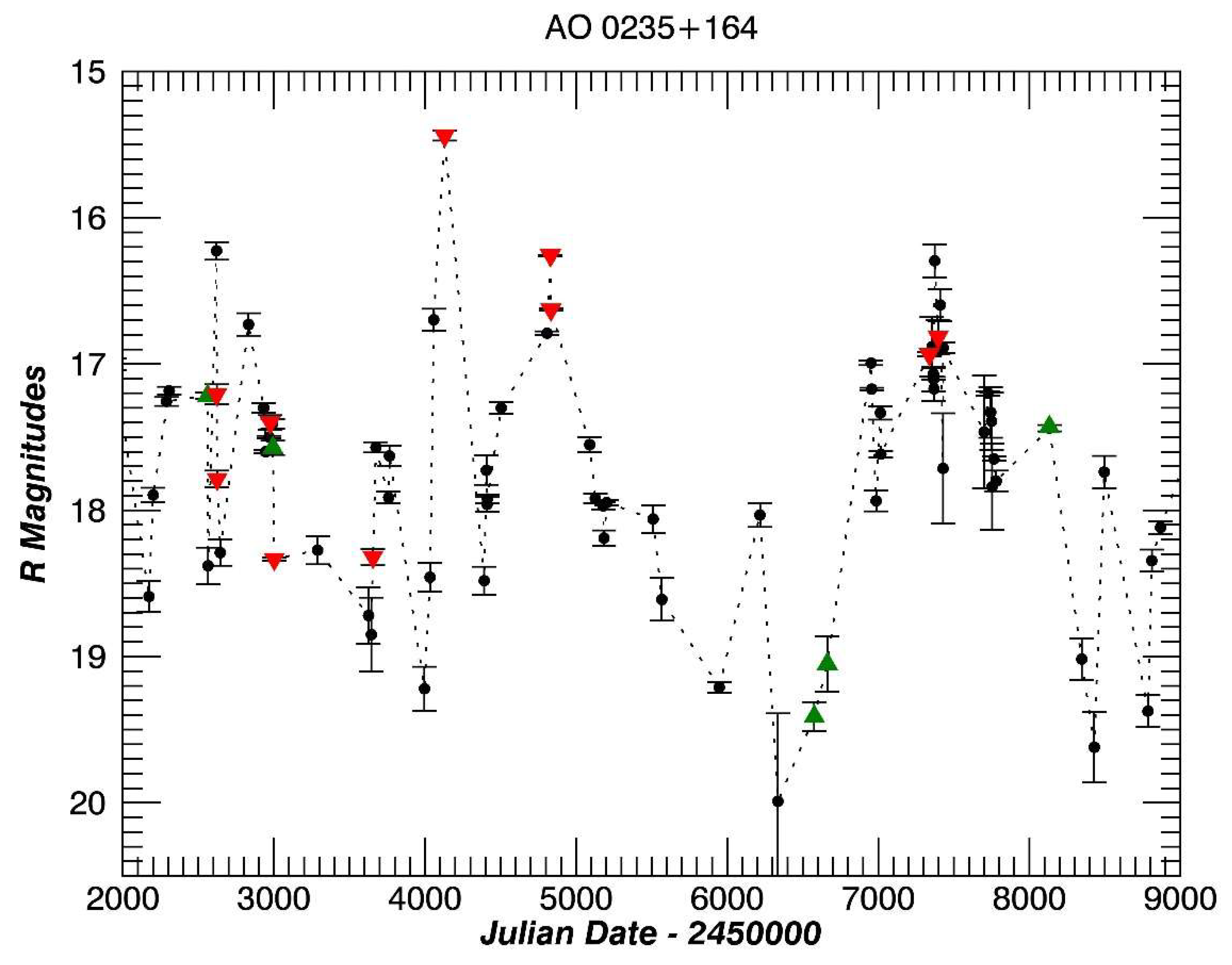
3.1. AO 0235+164
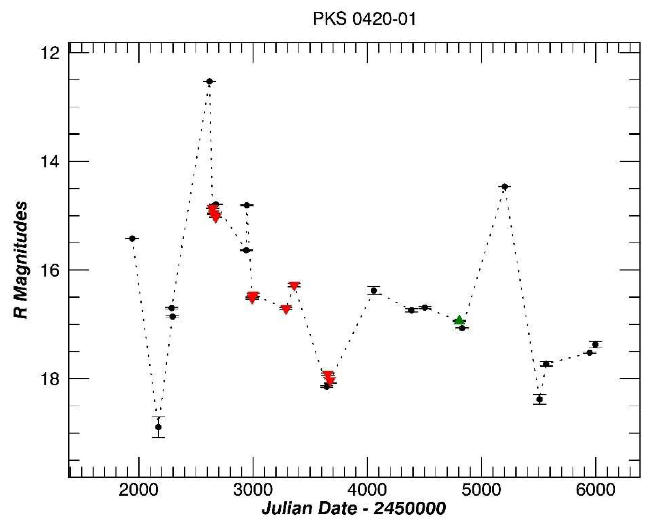
3.2. PKS 0420-01
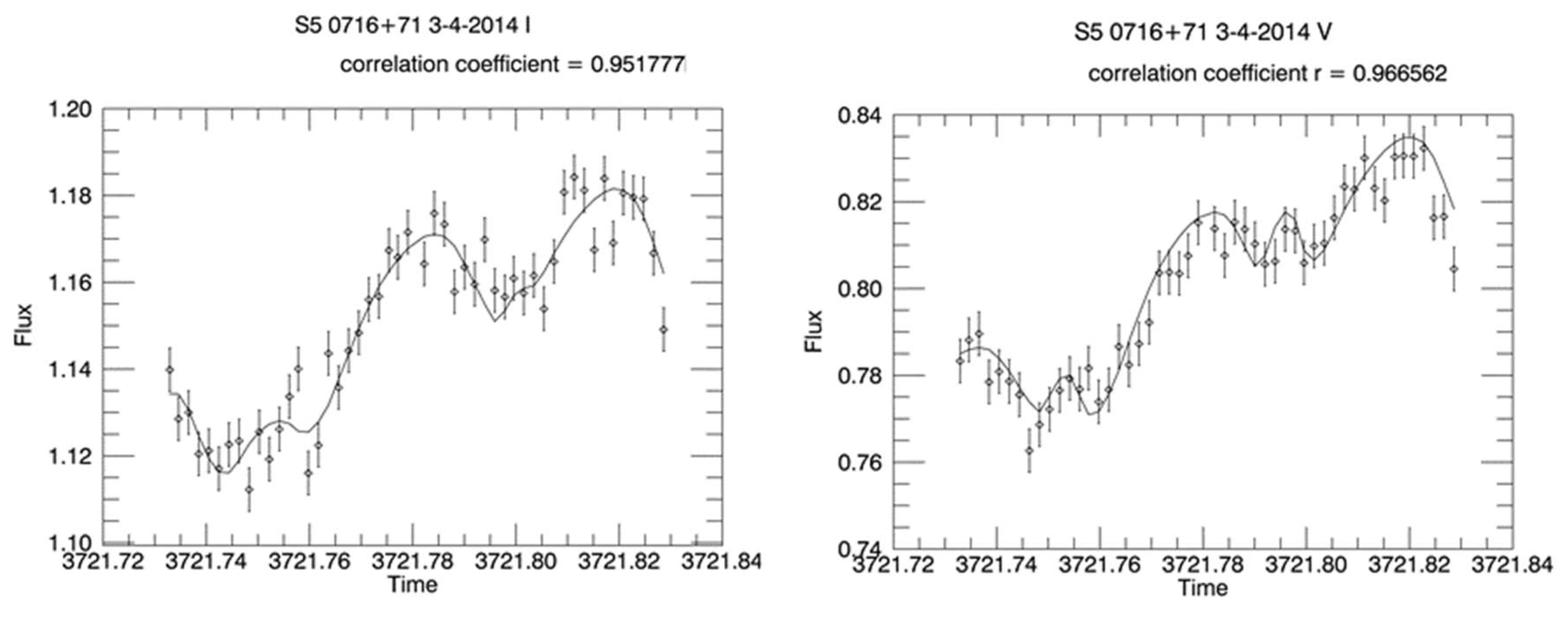
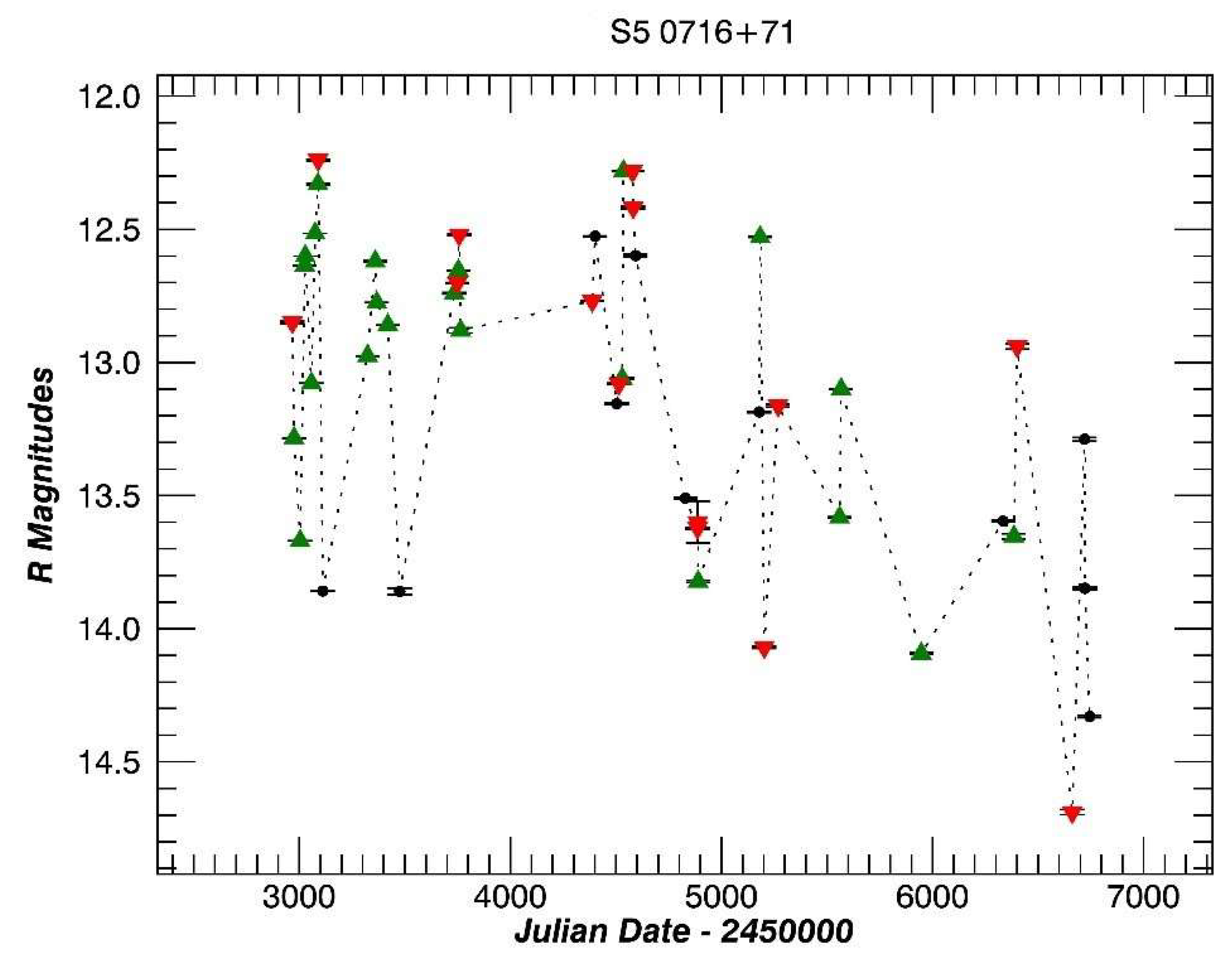
3.3. S5 0716+71
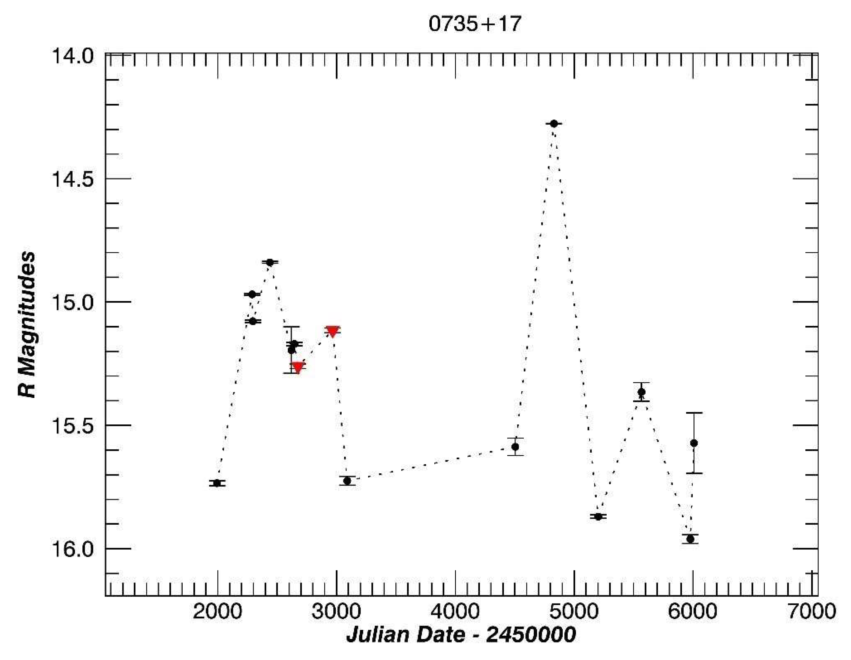
3.4. PKS 0735+17
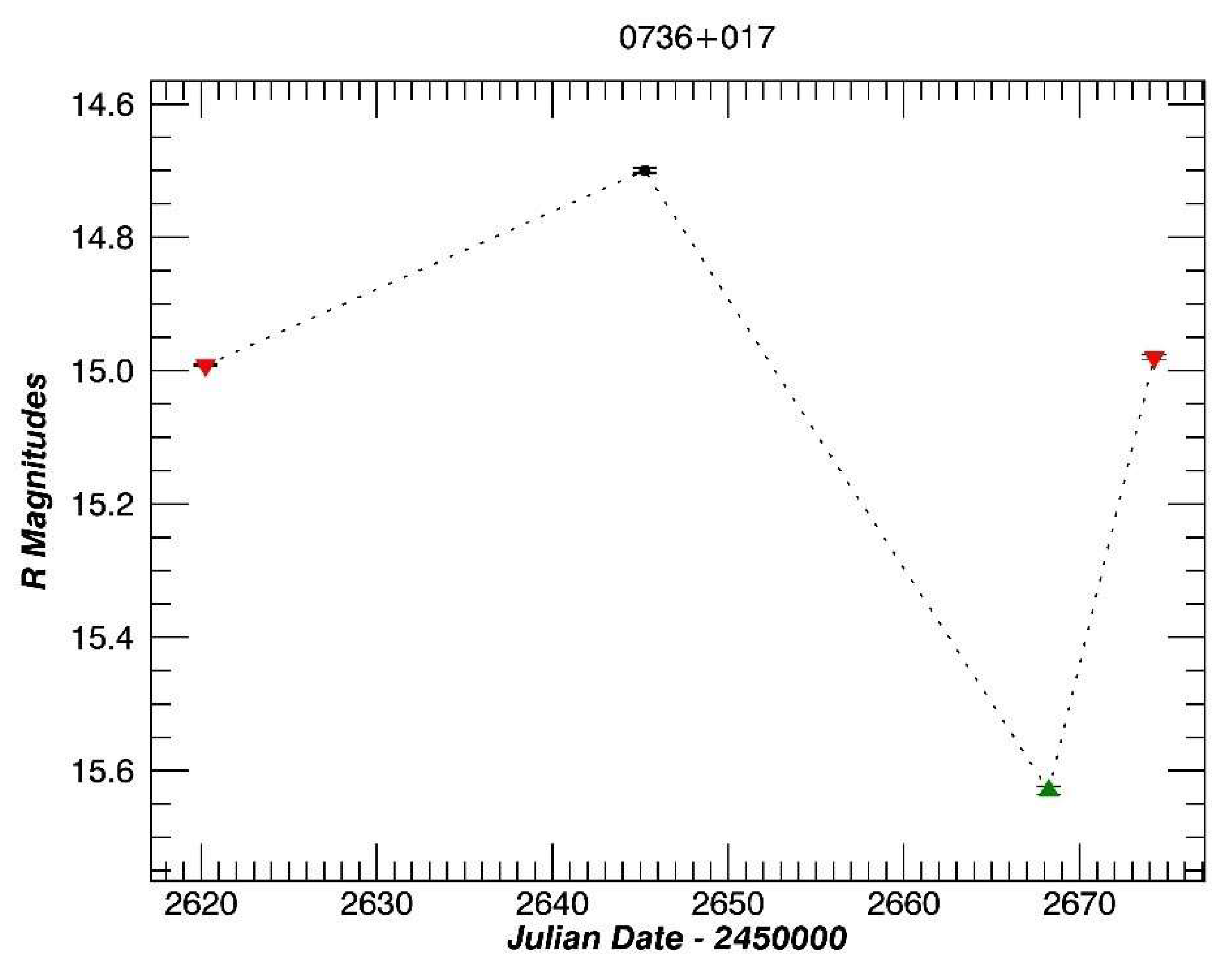
3.5. PKS 0736+071
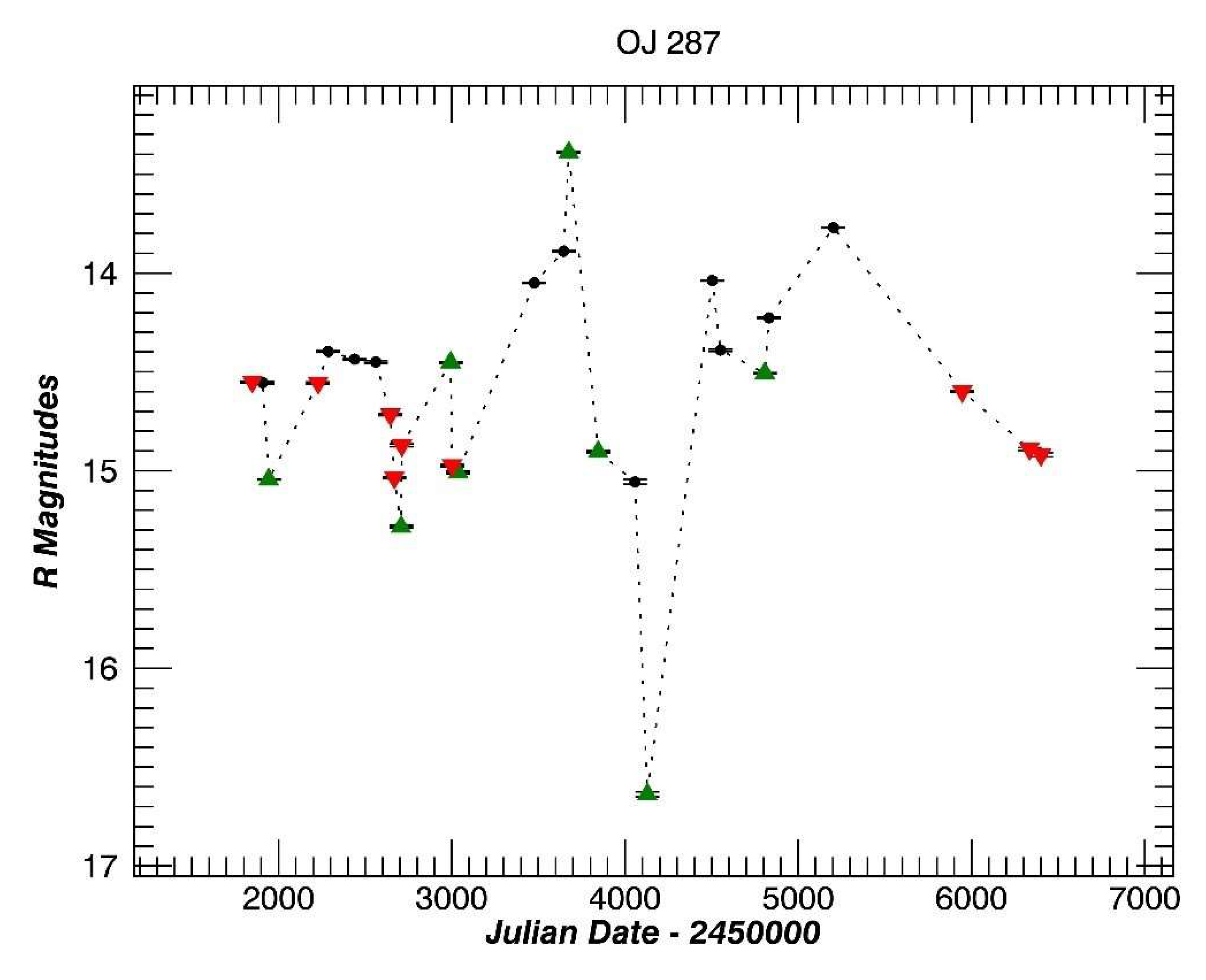
3.6. OJ 287
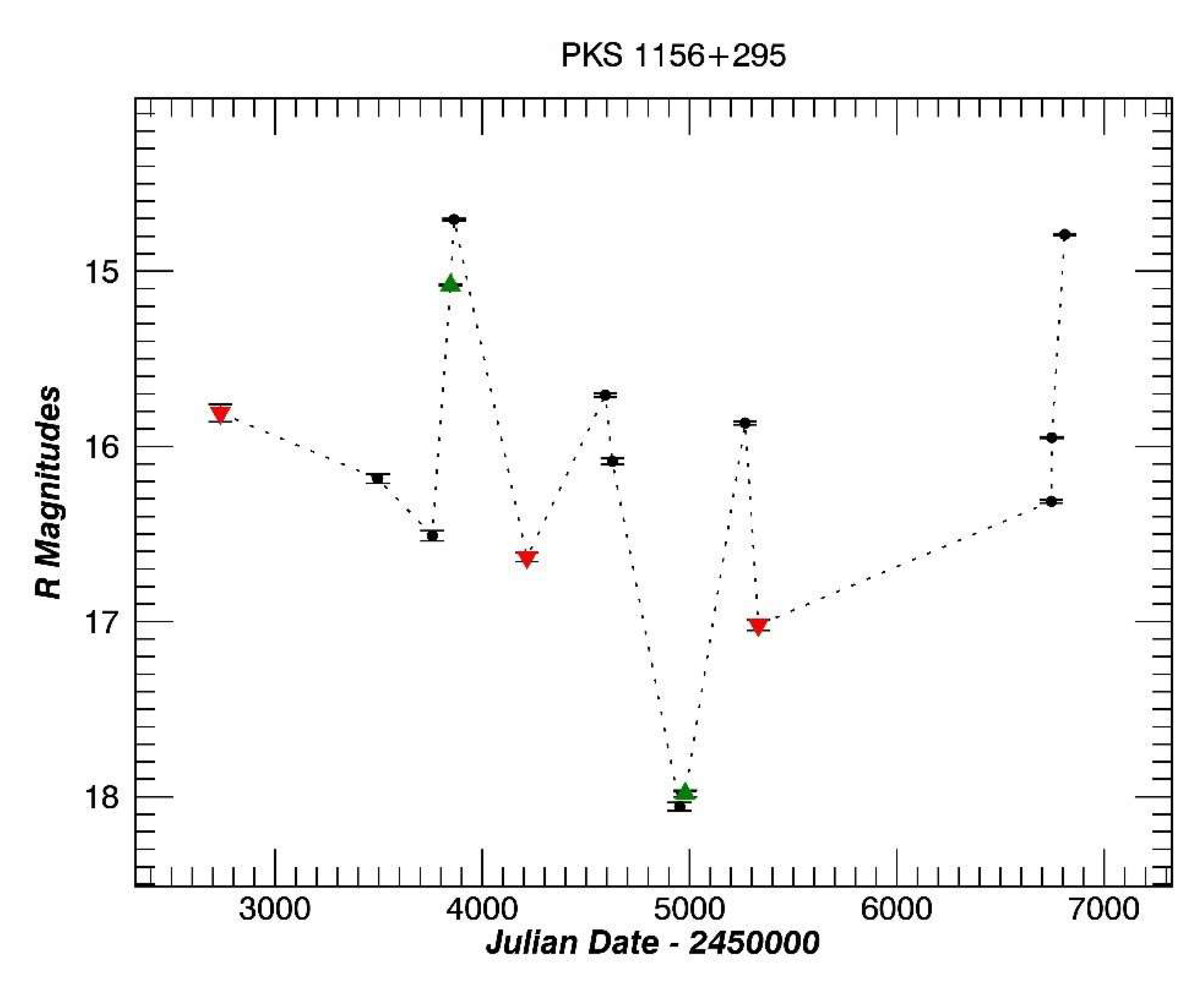
3.7. PKS 1156+295
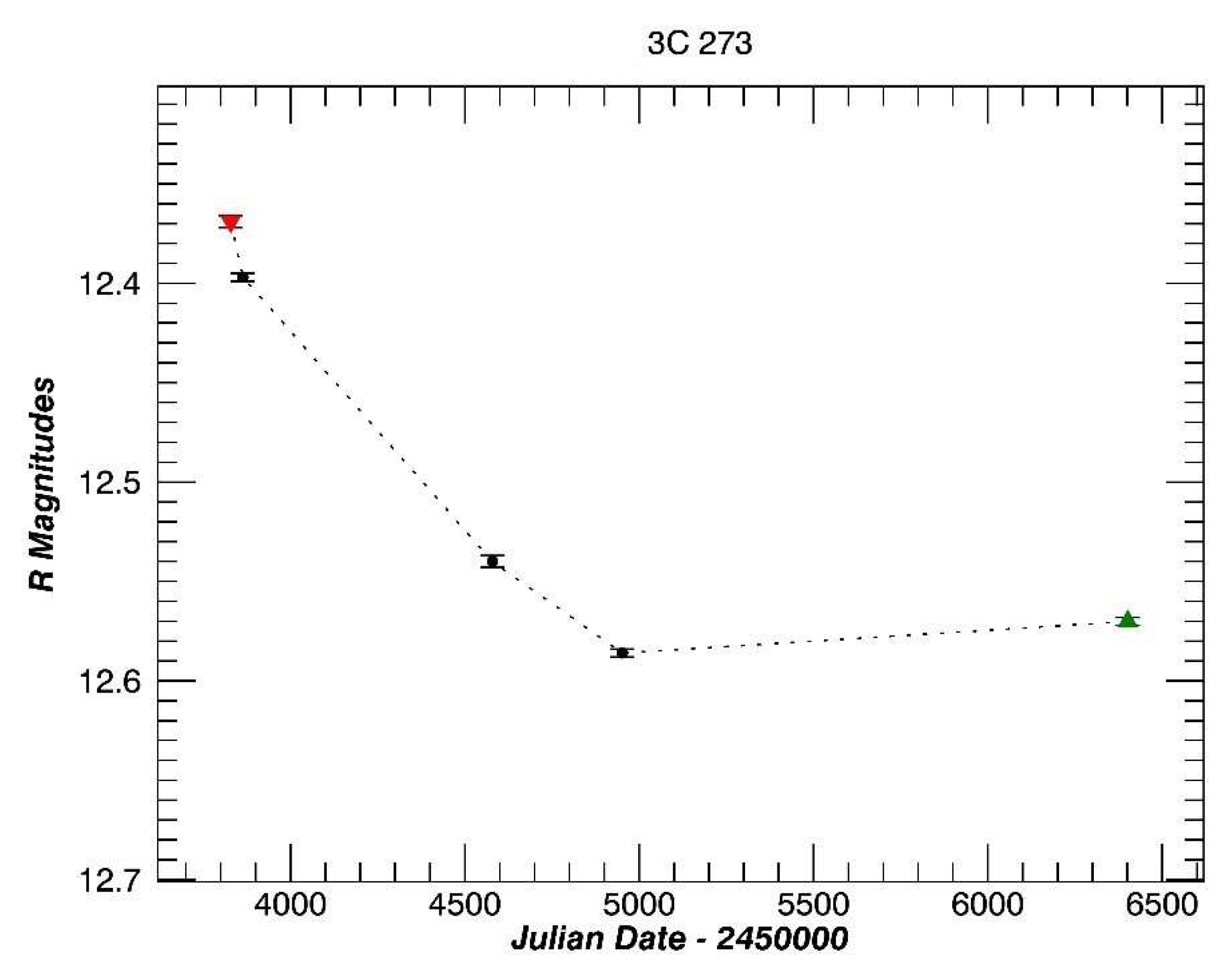
3.8. 3C 273
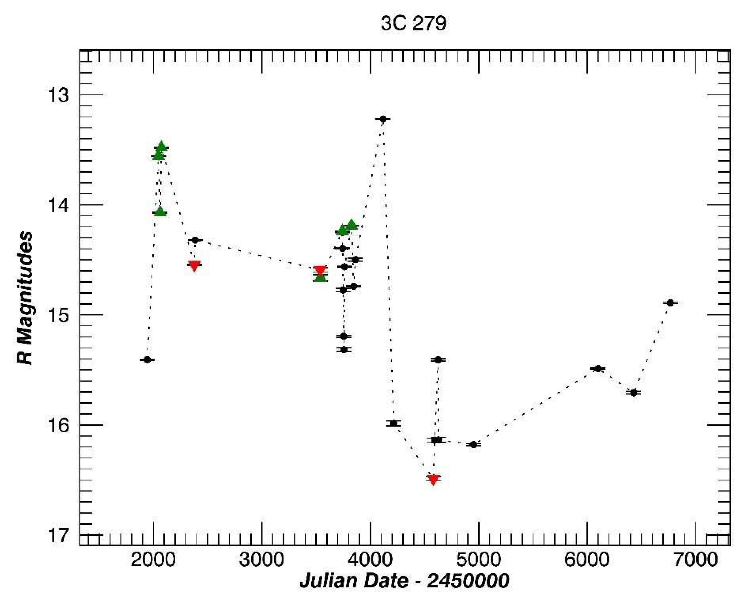
3.9. 3C 279
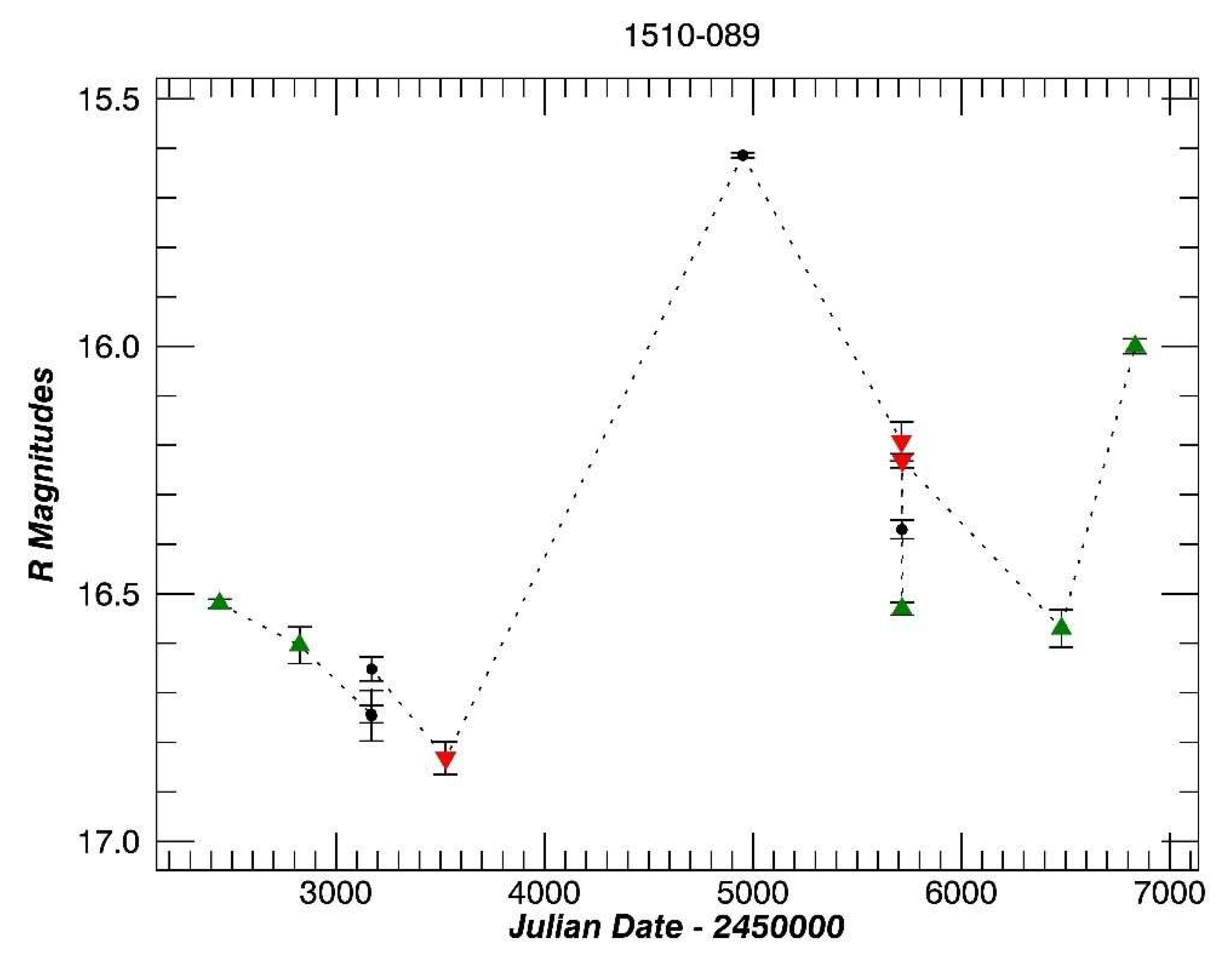
3.10. PKS 1510-089
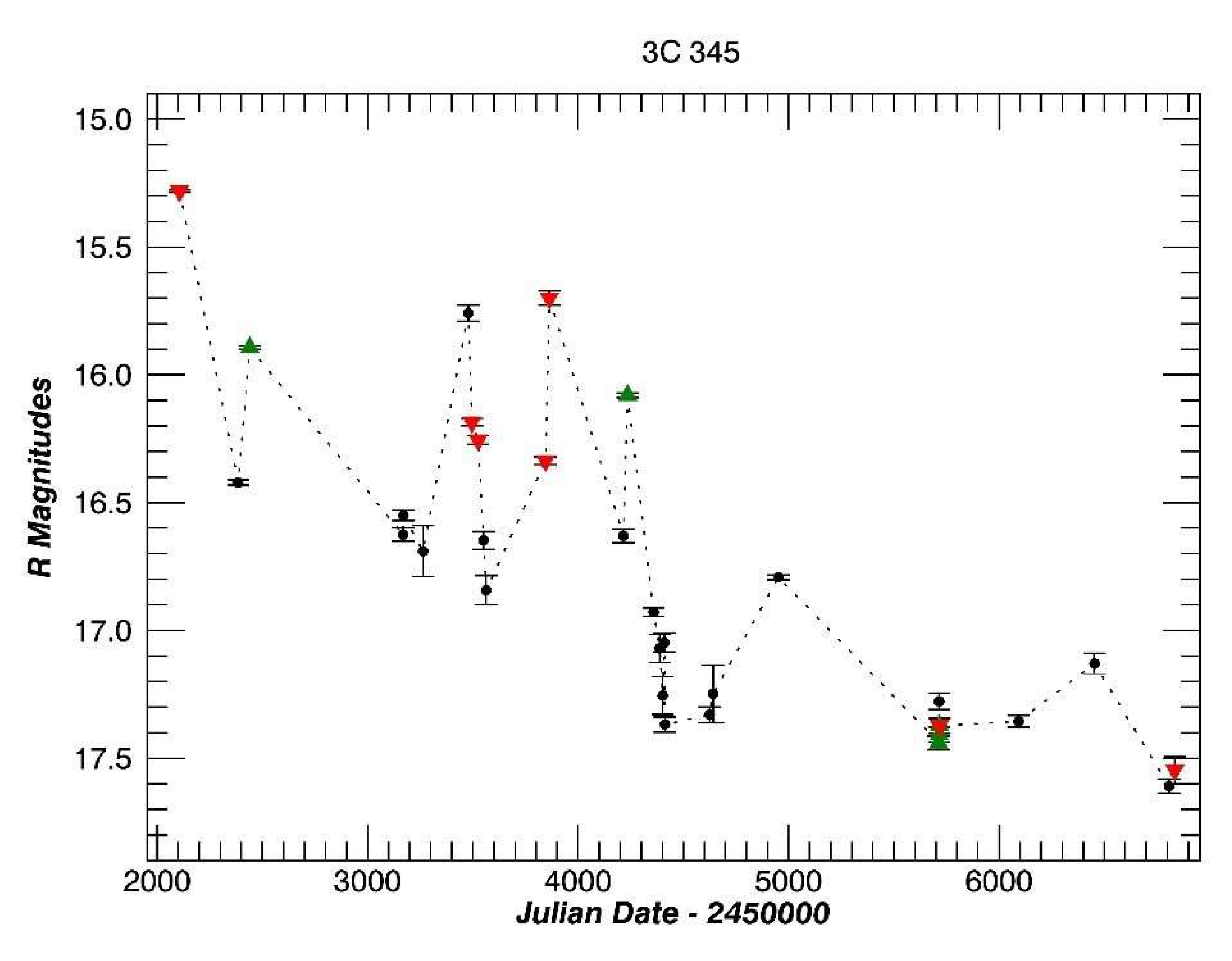
3.11. 3C 345
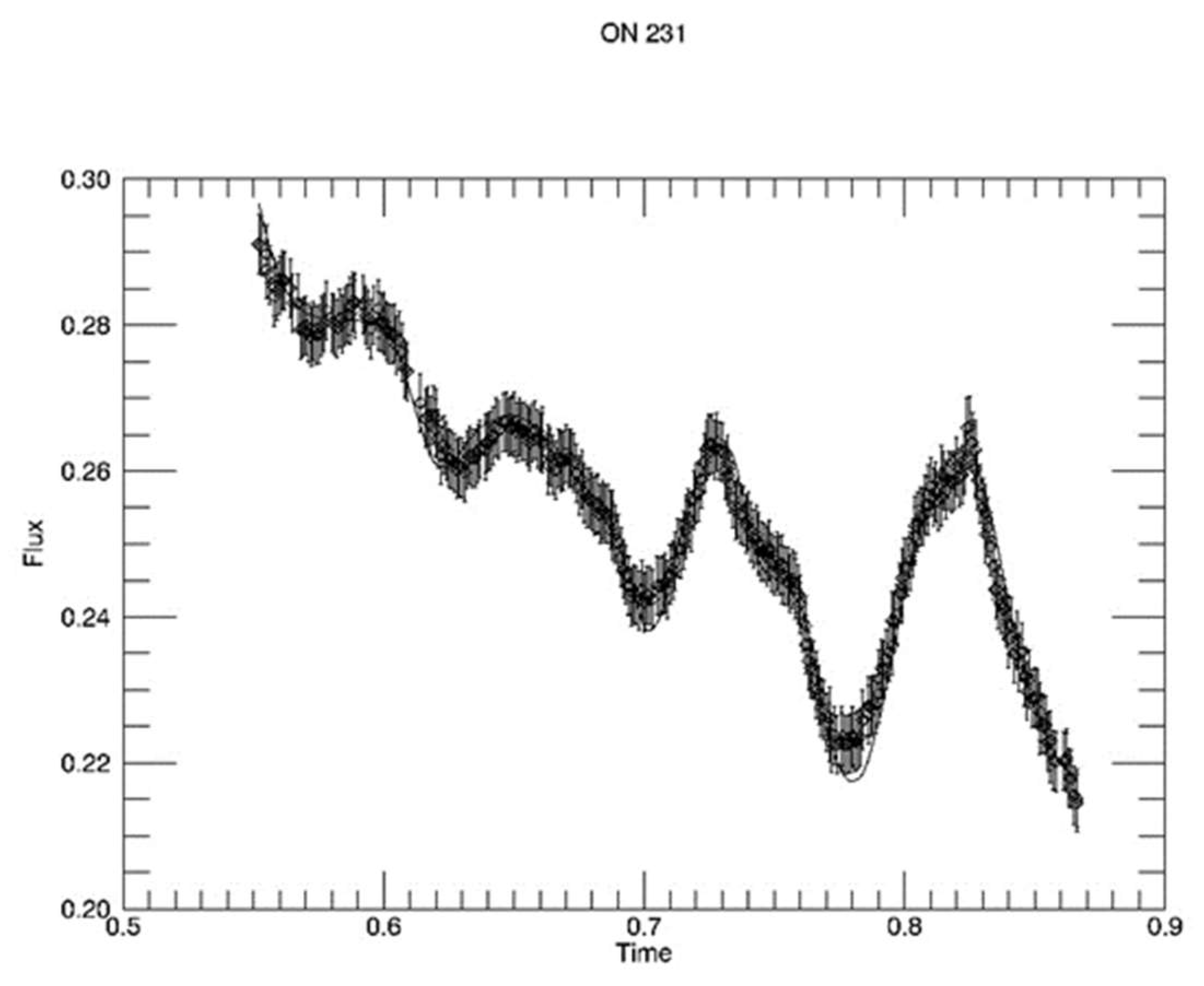
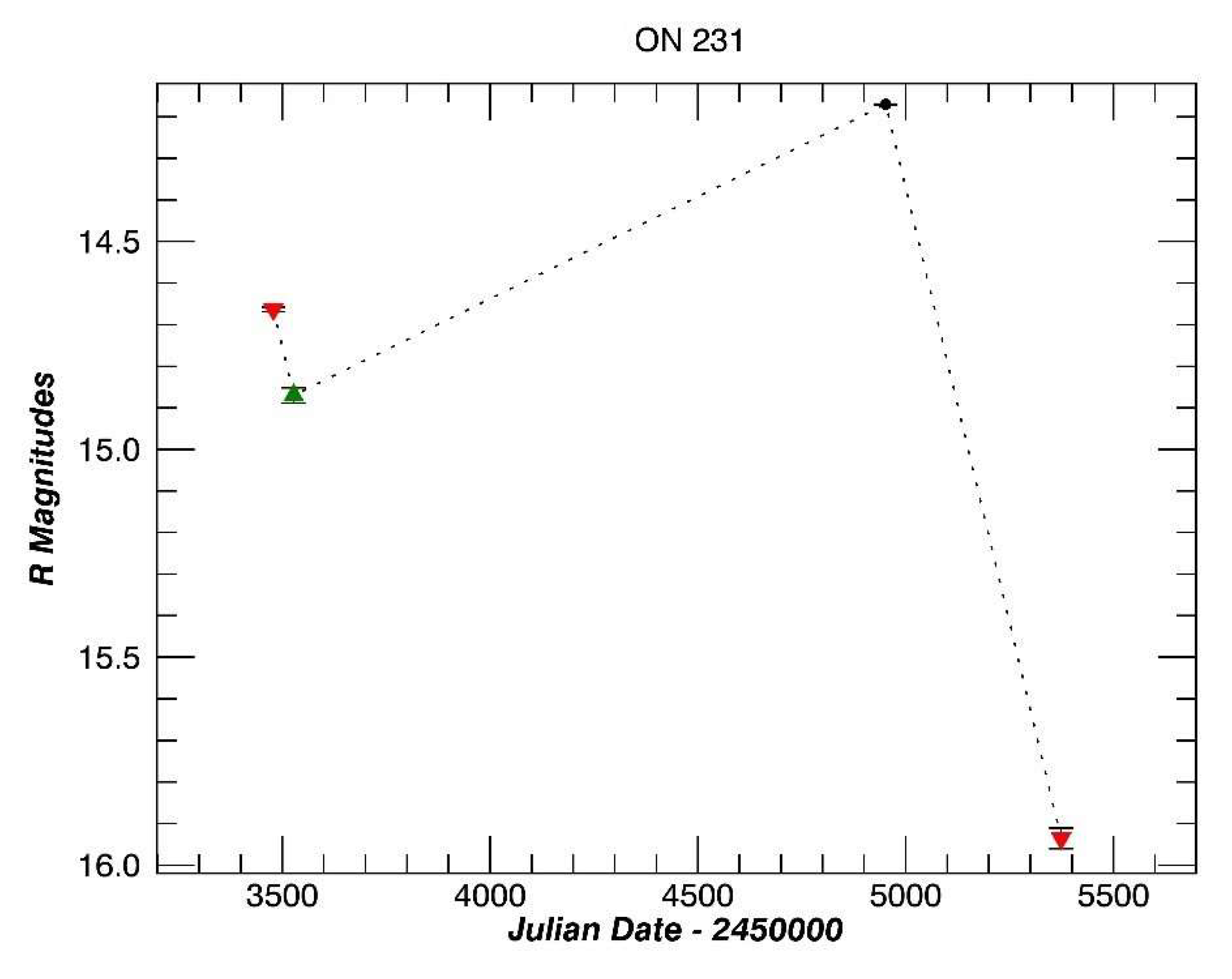
3.12. ON 231
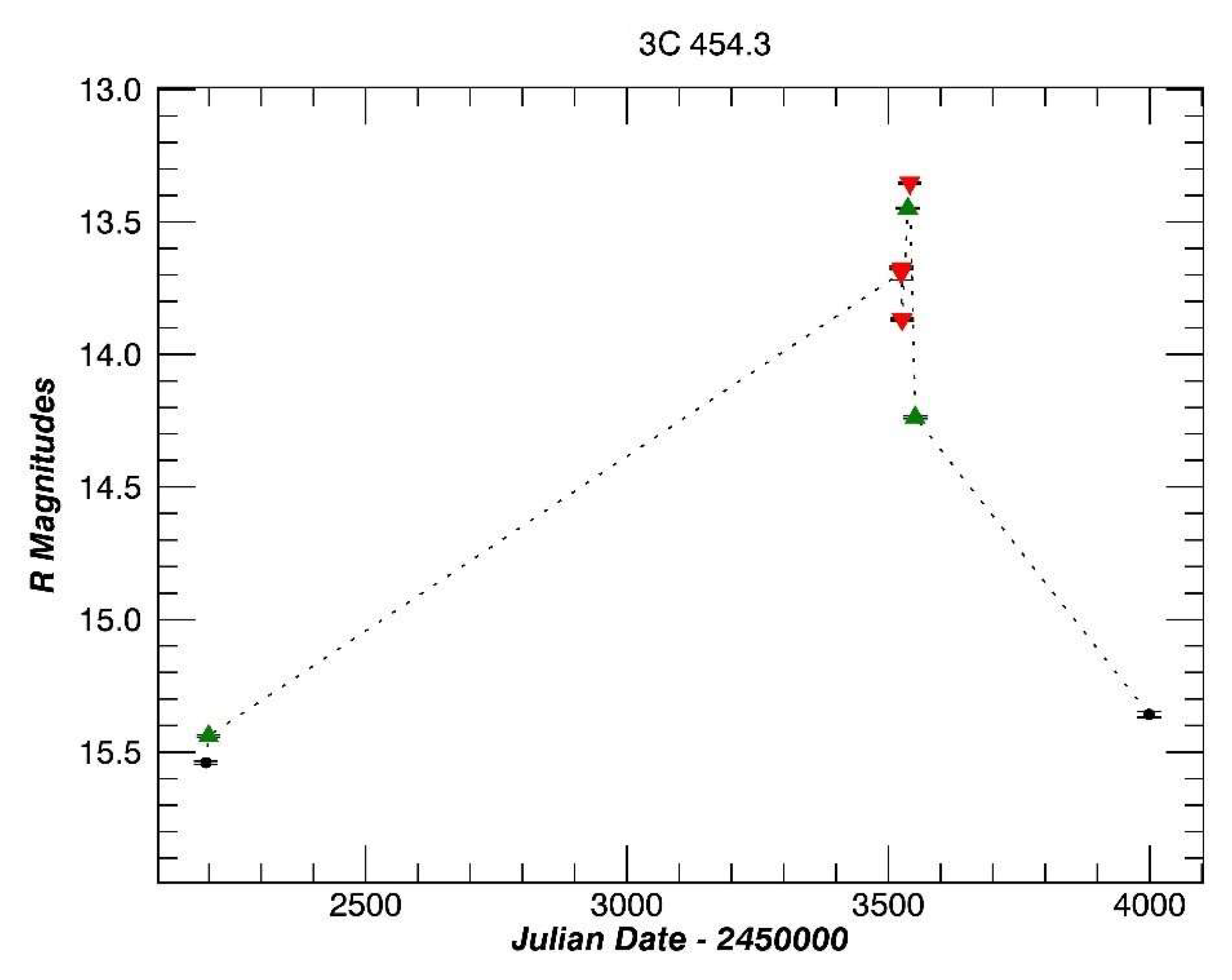
3.13. 3C 454.3
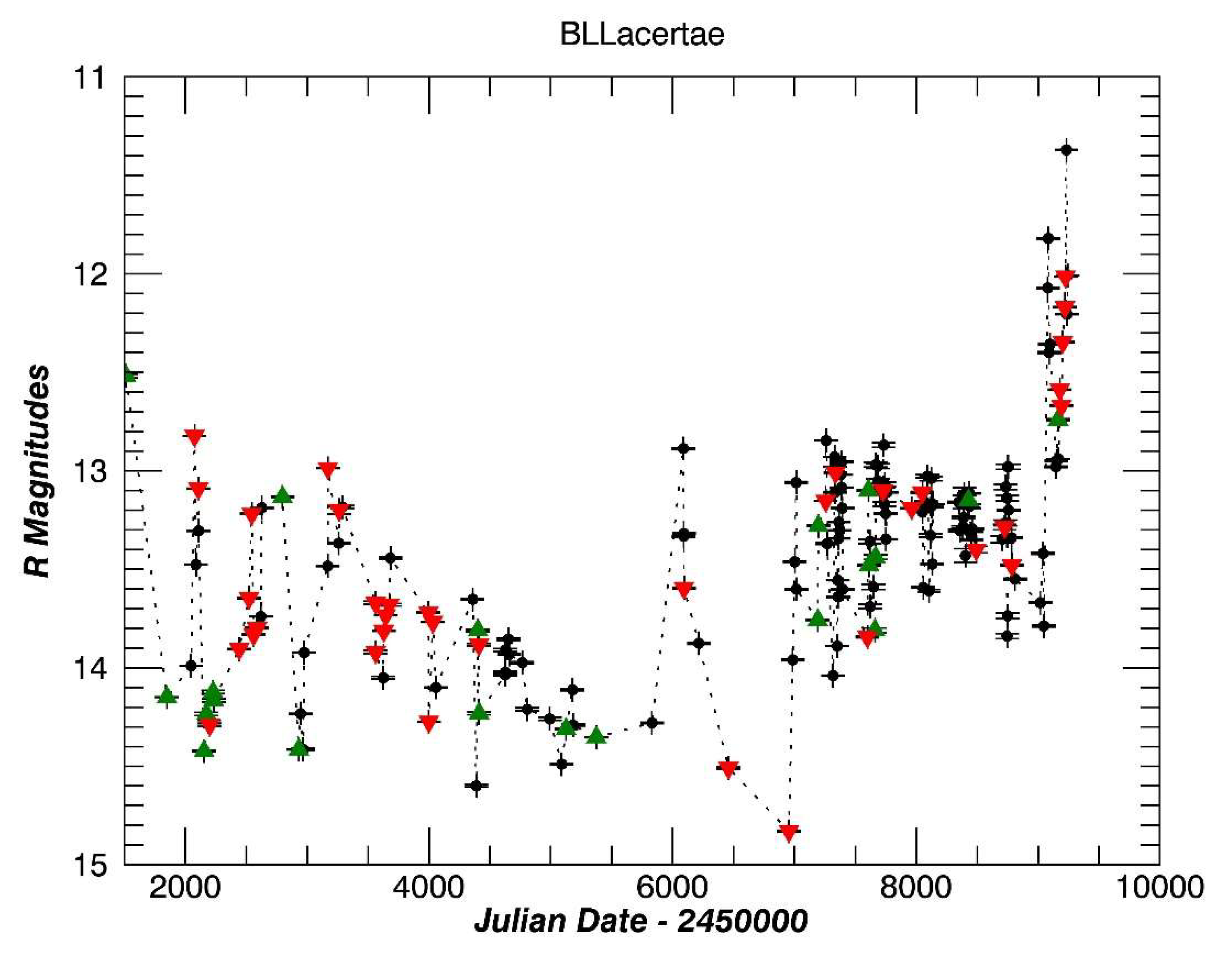
3.14. BL Lac
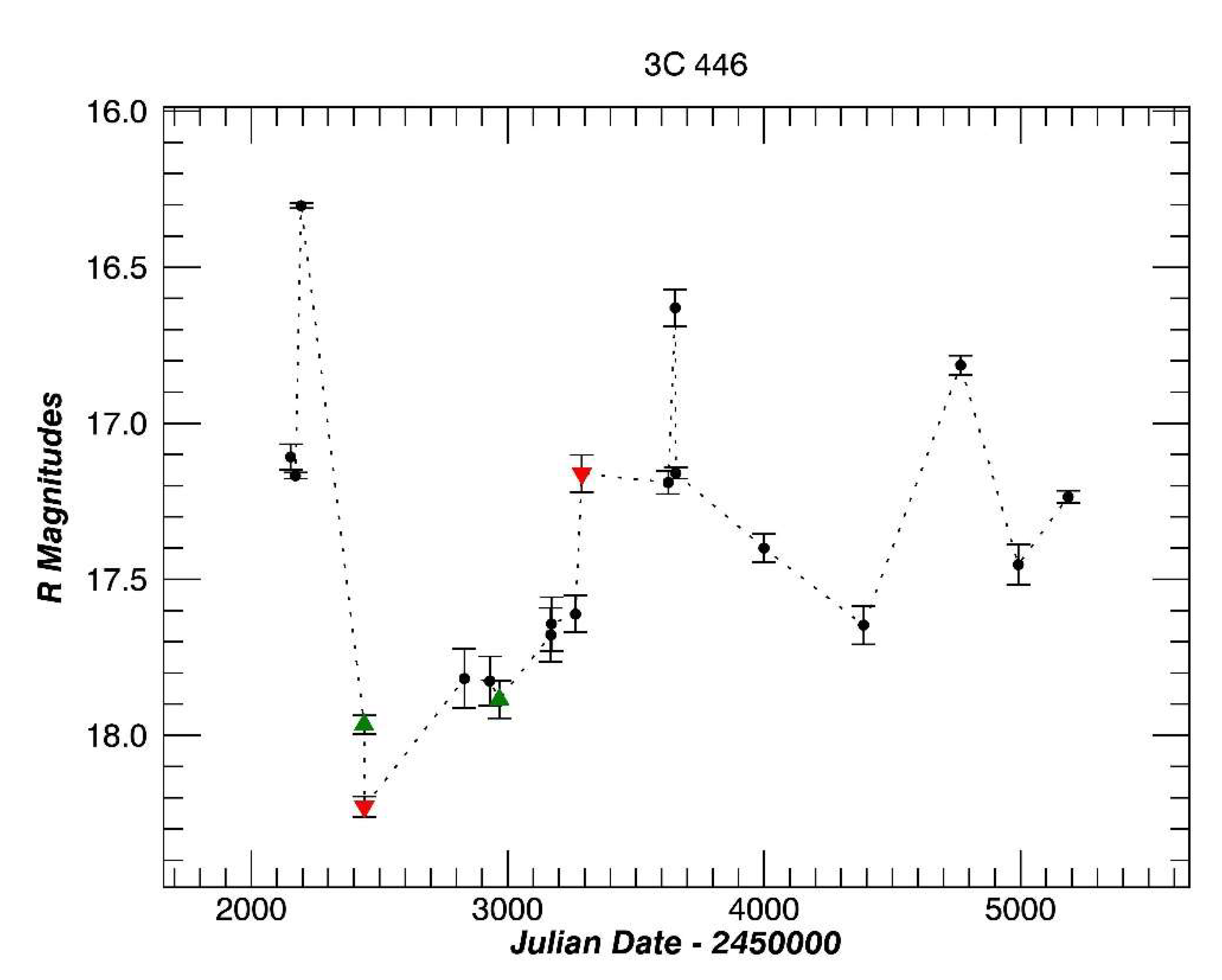
3.15. 3C446
4. Observational Results
4.1. Correlation with Flux Level
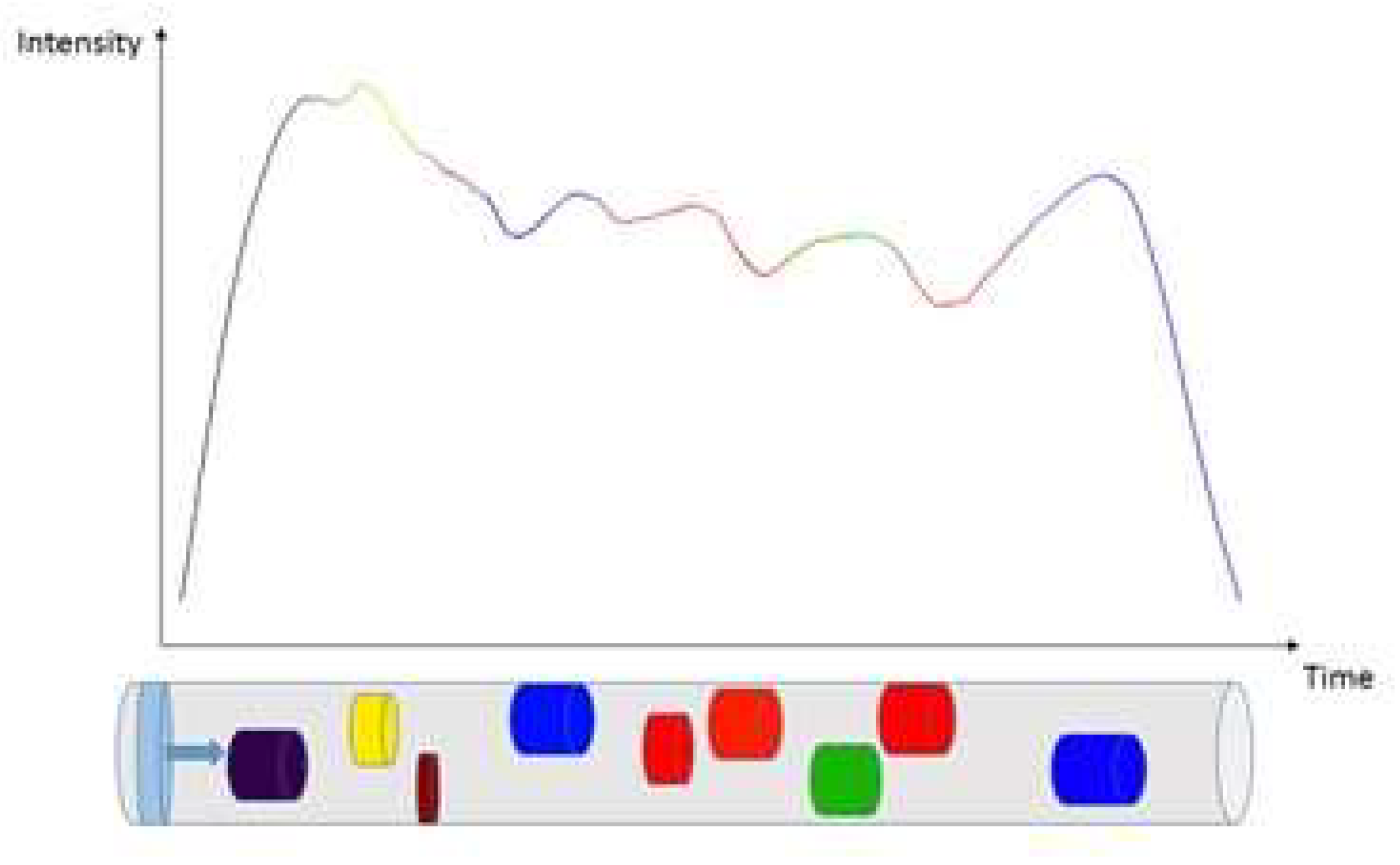
4.2. Theory of Shock Waves Encountering Turbulent Cells
- The occurrence of micro-variations showed no correlation with flux levels;
- Micro-variability is intermittent in each source;
- No consistent underlying periods were found in the micro-variations from one light curve to the next for any object;
5. Theoretical Model
5.1. Theory of Shock Waves Encountering Turbulent Cells
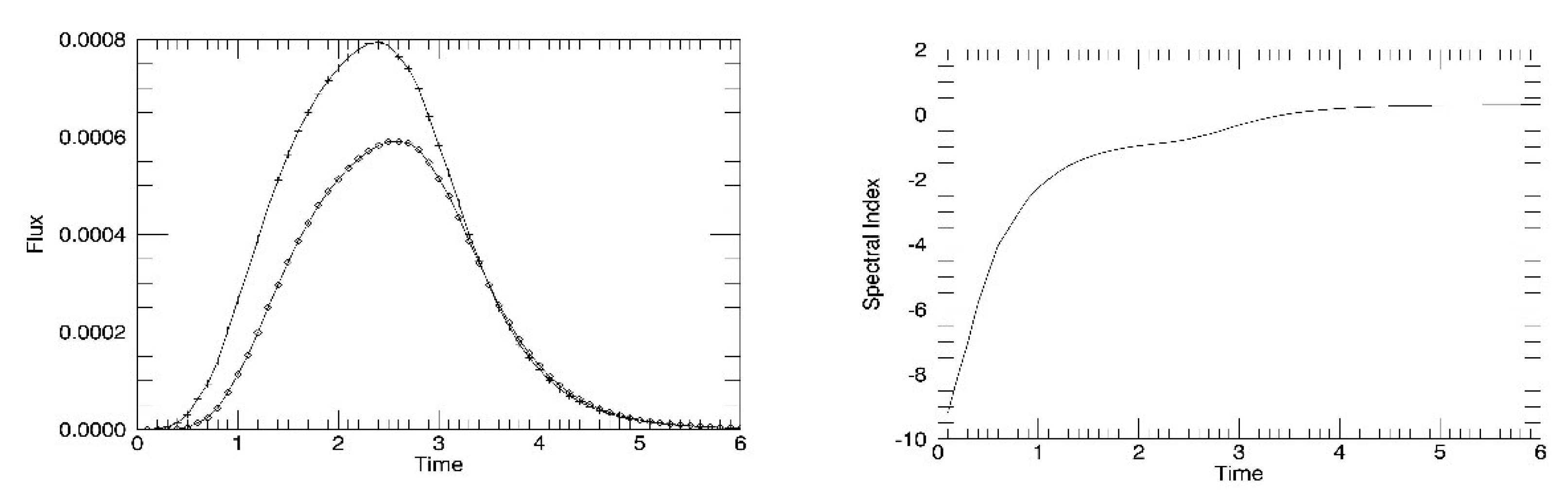
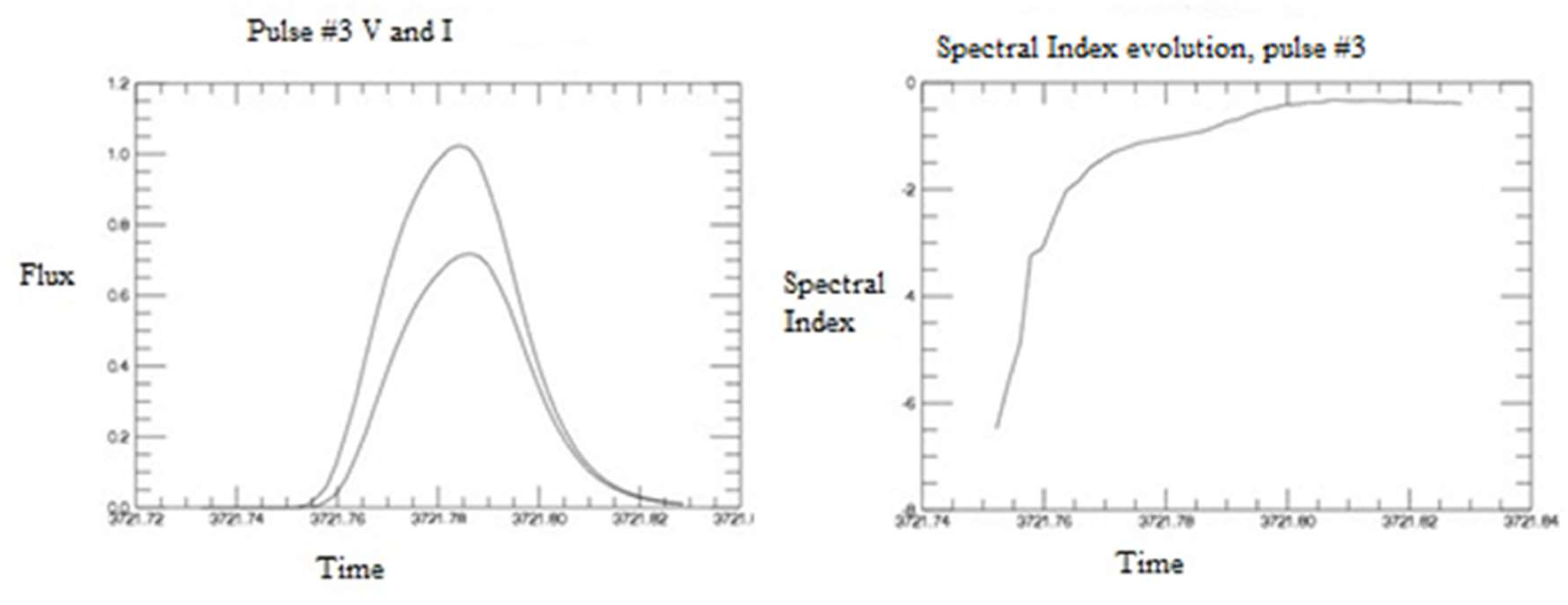
5.2. Fitting Pulse Profiles
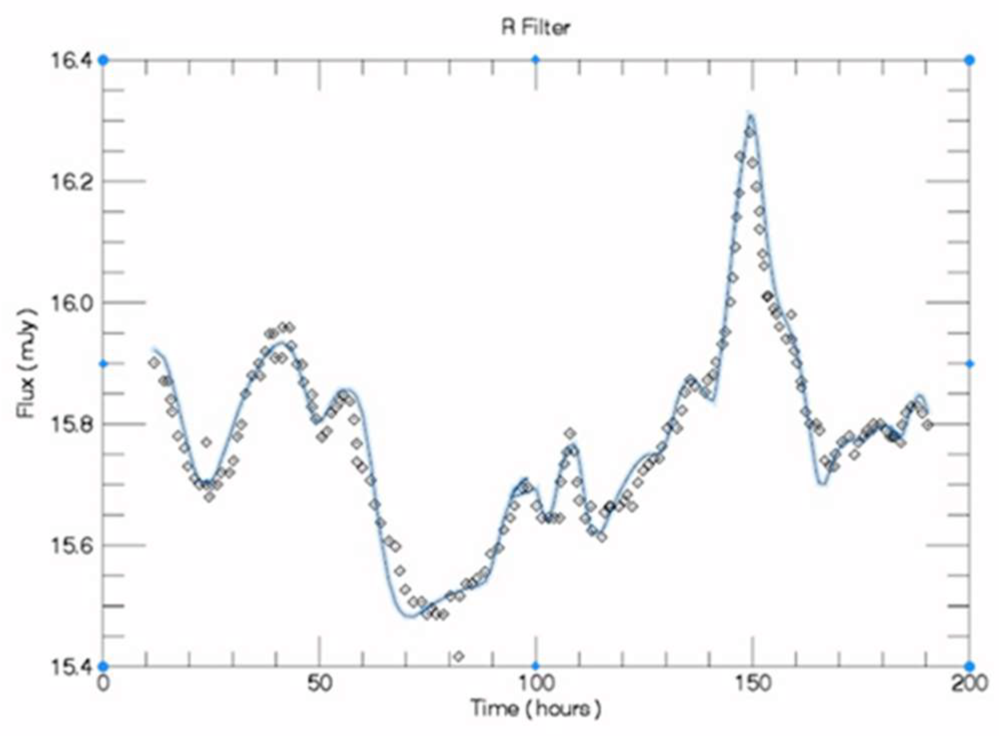
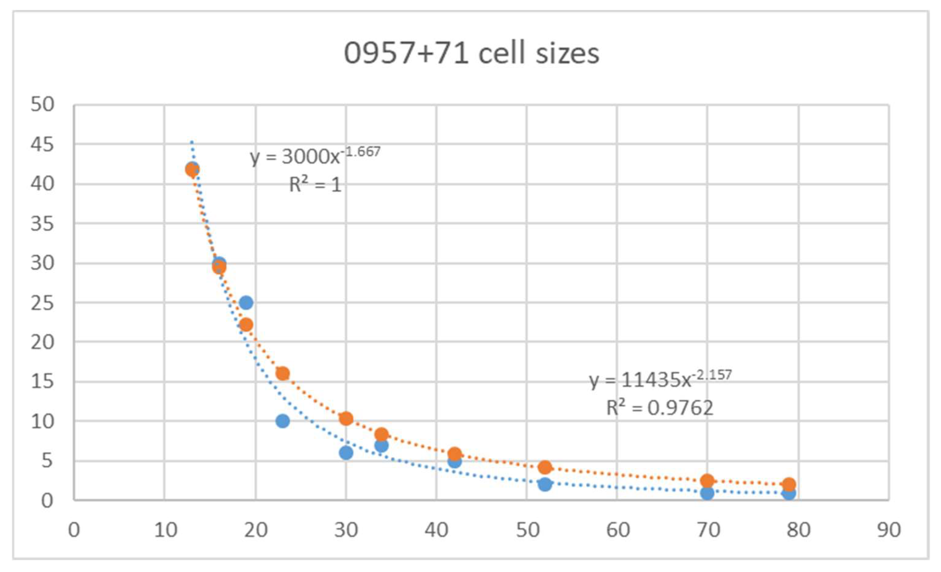
5.3. Testing the Model
5.4. Polarization Predictions and Test
6. Conclusions
Author Contributions
Funding
Institutional Review Board Statement
Informed Consent Statement
Data Availability Statement
Acknowledgments
Conflicts of Interest
Appendix A


References
- Webb, J.R.; Smith, A.G.; Leacock, R.J.; Fitzgibbons, G.L.; Gombola, P.P.; Shepard, D.W. Optical observations of 22 violently variable extragalactic sources-1968-1986. Astron. J. 1988, 95, 374. [Google Scholar] [CrossRef]
- Pollock, J.T.; Webb, J.; Azarnia, G. Simultaneous Microvariability Observations of 0716+ 71. Astron. J. 2007, 133, 487. [Google Scholar] [CrossRef]
- Qian, B.; Tao, J.; Fan, J. Optical Monitoring of S5 0716+ 714 from 1994 to 2000. Astrophys. J. 2002, 123, 678–689. [Google Scholar] [CrossRef]
- Howard, E.S.; Webb, J.R.; Pollock, J.T.; Branly, R.M.; Stencel, R.E. Microvariability and long-term variability of four blazars. Astron. J. 2004, 127, 17. [Google Scholar] [CrossRef]
- Montagni, F.; Maselli, A.; Massaro, E.; Nesci, R.; Sclavi, S.; Maesano, M. The intra-night optical variability of the bright BL Lacertae object S5 0716+ 714. Astron. Astrophys 2006, 451, 435. [Google Scholar] [CrossRef]
- Webb, J.R. Micro-variability of Blazars: Correlations and Duty Cycles. BAAS 2007, 210, 0202W. [Google Scholar]
- Webb, J.R. Multi-Frequency Blazar Micro-Variability as a Tool to Investigate Relativistic Jets. Galaxies 2016, 4, 15. [Google Scholar] [CrossRef]
- Wilkat, V.; Webb, J.R.; Clements, S.; Pollock, J.T. Time Series Analysis of Microvariability in Blazars. BAAS 2002, 34, 1179. [Google Scholar]
- Humrickhouse, C.; Webb, J. Wavelet Analysis of Microvariability in Blazars 0716+ 714, ON231 and BL Lac. JSARA 2008, 2, 23H. [Google Scholar]
- Jones, T.W. Polarization as a probe of magnetic field and plasma properties of compact radio sources-Simulation of relativistic jets. Astrophys. J. 1988, 332, 678. [Google Scholar] [CrossRef]
- Marscher, A.P. Turbulent, extreme multi-zone model for simulating flux and polarization variability in blazars. Astrophys. J. 2014, 780, 87. [Google Scholar] [CrossRef]
- Zrake, J.; MacFadyen, A.I. Numerical simulations of driven relativistic magnetohydrodynamic turbulence. Astrophys. J. 2011, 744, 32. [Google Scholar] [CrossRef]
- She, Z.; Leveque, E. Universal scaling laws in fully developed turbulence. Phys. Rev. Lett. 1994, 72, 336. [Google Scholar] [CrossRef]
- Marscher, A.P.; Jorstad, S.G. Frequency and Time Dependence of Linear Polarization in Turbulent Jets of Blazars. Galaxies 2021, 9, 27. [Google Scholar] [CrossRef]
- Bhatta, G.; Webb, J.R.; Hollingsworth, H.; Dhalla, S.; Khanuja, A.; Bachev, R.; Blinov, D.A.; Böttcher, M.; Bravo Calle, O.J.A.; Calcidese, P.; et al. The 72-h WEBT microvariability observation of blazar S5 0716 + 714 in 2009. Astron. Astrophys 2013, 558, A92. [Google Scholar] [CrossRef]
- Keel, W.; Oswalt, T.; Mack, P.; Henson, G.; Hilwig, T.; Bacheldor, D.; Berrrington, R.; DePree, C.; Hartmann, D.; Leake, M.; et al. Corrigendum: The Remote Observatories of the Southeastern Association for Research in Astronomy (SARA). PSAO 2021, 133, 1024. [Google Scholar] [CrossRef]
- Webb, J.R.; Barnello, T.; Robson, I.; Hartman, R.C. PKS 1156+ 295. IAU Circ. 1995, 6168, 1. [Google Scholar]
- Webb, J.R.; Freedman, I.; Howard, E.; Belfort, M.; Rave, H.; Krick, J.; Rumstay, K.; Nicol, S.; Oswalt, T.D. Broadband optical observations of BL lacertae during the 1997 outburst. Astron. J. 1998, 115, 2244. [Google Scholar]
- Finding Charts for AGN. Available online: https://www.lsw.uni-heidelberg.de/projects/extragalactic/charts/ (accessed on 10 February 2021).
- Böttcher, M.; Basu, S.; Joshi, M.; Villata, M.; Arai, A.; Aryan, N.; Asfandiyarov, I.M.; Bach, U.; Bachev, R.; Berduygin, A.; et al. The WEBT Campaign on the Blazar 3C 279 in 2006. Astrophys. J. 2007, 670, 968B. [Google Scholar]
- Bhatta, G.; Goyal, A.; Ostrowski, M.; Stawarz, Ł.; Akitaya, H.; Arkharov, A.A.; Bachev, R.; Benítez, E.; Borman, G.A.; Carosati, D.; et al. Discovery of a Highly Polarized Optical Microflare in Blazar S5 0716+714 during the 2014 WEBT Campaign. Astrophys. J. 2015, 809, L27. [Google Scholar] [CrossRef]
- Howell, S.; Mitchell, K.; Warnock, A. Statistical error analysis in CCD time-resolved photometry with applications to variable stars and quasars. Astron. J. 1988, 95, 147–256. [Google Scholar] [CrossRef]
- Tuorla Monitoring Program. 10 September. Available online: http://www.astro.bas.bg/~bachevr/blazar/tuorla.html (accessed on 10 September 2021).
- Webb, J.R.; Simth, A.G. The 1987 outburst of the BL Lacertid AO 0235+ 164. Astron. Astrophys. 1989, 220, 65. [Google Scholar]
- Raiteri, C.M.; Villata, M.; Ibrahimov, M.A.; Larionov, V.M.; Kadler, M.; Aller, M.F.; Kovalev, Y.Y.; Lanteri, L.; Nilsson, K.; Papadakis, I.E.; et al. The WEBT campaign to observe AO 0235+ 16 in the 2003–2004 observing season-Results from radio-to-optical monitoring and XMM-Newton observations. Astron. Astrophys. 2005, 438, 39–53. [Google Scholar] [CrossRef]
- Webb, J.R.; Howard, E.; Benitez, E.; Bslonek, T.; McGrath, E.; Shrader, C.; Robson, I.; Jenkins, P. The 1997 outburst of AO 0235+ 164: Evidence for a microlensing event? Astron. J. 2000, 120, 41. [Google Scholar] [CrossRef]
- Raiteri, C.M.; Villata, M.; Kadler, M.; Ibrahimov, M.A.; Kurtanidze, O.M.; Larionov, V.M.; Tornikoski, M.; Boltwood, P.; Lee, C.-U.; Aller, M.F.; et al. Multifrequency variability of the blazar AO 0235+ 164-The WEBT campaign in 2004–2005 and long-term SED analysis. Astron. Astrophys. 2006, 459, 731–743. [Google Scholar] [CrossRef]
- Ghosh, K.; Chulhee, K.; Ramsey, B.D.; Soundaperumal, S. Optical Microvariability of Blazars. JKAS...34....9GJ. 2001, 34, 9. [Google Scholar]
- Dai, B.Z.; Xie, G.Z.; Li, K.H.; Zhou, S.B.; Liu, W.W.; Jiang, Z.J. Rapid optical variability of gamma-ray-loud blazars. Astron. J. 2001, 122, 2901. [Google Scholar] [CrossRef]
- Xie, G.Z.; Li, K.H.; Bai, J.M.; Dai, B.Z.; Liu, W.W.; Zhang, X.; Xing, S.Y. Search for short variability timescale of the GEV gamma-ray-loud blazars. Astrophys. J. 2001, 548, 200. [Google Scholar] [CrossRef]
- Sagar, R.; Gopal-Krishna, M.V.; Pandey, A.; Bhatt, B.; Wagner, S. Multi-colour optical monitoring of the intra-day variable blazar S5 0716+ 71. Astron. Astrophys. Suppl. Ser. 1999, 134, 453–461. [Google Scholar] [CrossRef]
- Villata, M.; Mattox, J.R.; Massaro, E.; Nesci, R.; Catalano, S.; Frasca, A.; Raiteri, C.M.; Sobrito, G.; Tosti, G.; Nucciarelli, G.; et al. The 0716+ 714 WEBT campaign of February 1999. Astron. Astrophys. 2000, 363, 108–116. [Google Scholar]
- Nesci, R.; Massaro, E.; Rossi, C.; Sclavi, S.; Maesana, M.; Montagni, F. The long-term optical variability of the BL Lacertae object S5 0716+ 714: Evidence for a precessing jet. Astron. J. 2005, 130, 1466. [Google Scholar] [CrossRef]
- Villata, M.; Raiteri, C.M.; Larionov, V.M.; Kurtanidze, O.M.; Nilsson, K.; Aller, M.F.; Tornikoski, M.; Volvach, A.; Aller, H.D.; Arkharov, A.A.; et al. Multifrequency monitoring of the blazar 0716+ 714 during the GASP-WEBT-AGILE campaign of 2007. Astron. Astrophys. 2008, 481, L79–L82. [Google Scholar] [CrossRef]
- Carini, M.; Walters, R.; Hopper, L. Multicolor Optical Microvariability in S5 0716+ 714. Astron. J. 2011, 141, 49. [Google Scholar] [CrossRef]
- Bhatta, G.; Ostrwoski, M.; Stawarz, L.; Zola, S.; Jableka, D.; Bachev, R.; Benitez, E.; Dhalla, S.M.; Cason, A.; Carosati, D.; et al. 5-day photo-polarimetric WEBT Campaign on Blazar S5 0716+714—A Study of Microvariabiltiy in Blazar. AAS 2015, 665A, 7H. [Google Scholar]
- Bregman, J.; Glassgold, A.E.; Huggins, P.J.; Aller, H.D.; Aller, M.F.; Hodge, P.E.; Rieke, G.H.; Lebofsky, M.J.; Pollock, J.T.; Pica, A.J.; et al. Multifrequency observations of the BL Lacertae object 0735+ 178. Astrophys. J. 1984, 276, 454–465. [Google Scholar] [CrossRef]
- Sandrinelli, A.; Covino, S.; Treves, A. Long and short term variability of seven blazars in six near-infrared/optical bands. Astron. Astrophys. 2014, 562, A79. [Google Scholar] [CrossRef]
- Hartmann, R.C.; Webb, J.R.; Marscher, A.P.; Travis, J.P.; Dermer, C.D.; Aller, H.D.; Aller, M.F.; Balonek, T.J.; Bennett, K.; Bloom, S.D.; et al. Simultaneous Multiwavelength Spectrum and Variability of 3C 279 from 10 9 to 10 24 Hz. Astrophys. J. 1996, 461, 698. [Google Scholar] [CrossRef]
- Pollock, J.T. Short Time-Scale Pulsations in ON 231. BAAS 1999, 31, 1396. [Google Scholar]
- Sandage, A. Intensity Variations of Quasi-Stellar Sources in Optical Wavelengths. Astrophys. J. 1966, 144, 1234S. [Google Scholar] [CrossRef]
- Rateri, C.M.; Villata, M.; Larionov, V.M.; Pursimo, T.; Ibrahimov, M.A.; Nilsson, K.; Aller, M.F.; Kurtanidze, O.M.; Foschini, L.; Ohlert, J. WEBT and XMM-Newton observations of 3C 454.3 during the post-outburst phase-Detection of the little and big blue bumps. Astron. Astrophys. 2007, 473, 819. [Google Scholar] [CrossRef][Green Version]
- MacPherson, E.; Hasan, I.; Urry, M.; Buxton, M.; Bailyn, C.; Coppi, P.; Isler, J. Record O/IR Brightness of 3C 454.3. The Astronomer’s Telegram 2014, 6266, 1. [Google Scholar]
- Wu, J.; Peng, B.; Zhou, X.; Ma, J.; Jiang, Z.; Chen, J. Optical monitoring of BL Lacertae object S5 0716+ 714 with high temporal resolution. Astron. J. 2005, 129, 1818. [Google Scholar] [CrossRef]
- Fan, J.H.; Xie, G.Z.; Pecontal, E.; Pecontal, A.; Copin, Y. Historic light curve and long-term optical variation of BL Lacertae 2200+ 420. Astrophys. J. 1998, 507, 173–178. [Google Scholar] [CrossRef]
- Romero, G.E.; Cellone, S.A.; Combi, J.A. Optical microvariability of southern AGNs. Astron. Astrophys. Suppl. Ser. 1999, 135, 477. [Google Scholar] [CrossRef]
- Clements, S.D.; Carini, M.T. Multiband microvariability observations of BL lacertae during the outburst of 1997. Astron. J. 2001, 121, 90. [Google Scholar] [CrossRef]
- Lehto, H.A. Model for 1/F-TYPE Variability in Active Galactic Nuclei. In Proceedings of the 23rd ESLAB Symposium on Two Topics in X-Ray Astronomy, Bologna, Italy, 13–20 September 1989; Volume 2, p. 499. [Google Scholar]
- Kirk, J.; Reiger, F.M.; Mastichiadis, A. Particle acceleration and synchrotron emission in blazar jets. Astron. Astrophys. 1998, 333, 452. [Google Scholar]
- Ball, L.T.; Kirk, J.G. Diffusive acceleration of electrons in SN 1987A. Astrophys. J. 1992, 396, L39. [Google Scholar] [CrossRef]
- Zrake, J. Inverse cascade of nonhelical magnetic turbulence in a relativistic fluid. Astrophys. Lett. 2014, 794, L26. [Google Scholar] [CrossRef]
- Dhalla, S. Analysis of Kepler Active Galactic Nuclei Using A Revised Kirk, Rieger, Mastichiadis (1998) Model. Master’s Thesis, Florida International University, Miami, FL, USA. Available online: https://digitalcommons.fiu.edu/etd/1521/ (accessed on 10 January 2021).
- Rafle, H.; Webb, J.R.; Bhatta, G. Determining cell sizes in the Turbulent Jet of Blazar S5 0716+ 714. AAS 2013, 221, 33133924R. [Google Scholar]
- Xu, J.; Hu, S.; Jiang, Y.; Webb, J.R.; Bhatta, G.; Chen, X.; Alexeeva, S.; Li, Y. Statistical Analysis of Microvariability Properties of the Blazar S5 0716+ 714. Astrophys. J. 2019, 884, 92x. [Google Scholar] [CrossRef]
- Zrake, J. Private communication, 2018.
- Bhatta, G.; Webb, J.R. Microvariability in BL Lacertae:“Zooming” into the Innermost Blazar Regions. Galaxies 2018, 6, 2. [Google Scholar] [CrossRef]
- Meng, N.; Zhang, X.; Wu, J.; Ma, J.; Zhou, X. Multi-color Optical Monitoring of 10 Blazars from 2005 to 2011. Astrophys. Suppl. Ser. 2018, 237, 30M. [Google Scholar] [CrossRef]
- Weaver, Z.R.; Williamson, K.E.; Jorstad, S.G.; Marscher, A.P.; Larionov, V.M.; Raiteri, C.M.; Villata, M.; Acosta-Pulido, J.A.; Bachev, R.; Baida, G.V.; et al. Multiwavelength Variability of BL Lacertae Measured with High Time Resolution. Astophys. J. 2020, 900, 137. [Google Scholar] [CrossRef]
- Dhalla, S.; Webb, J.; Bhatta, G.; Lawrence, D. Analysis of Kepler Lightcurves Using Turbulent Jet Model. AAS Meeting 2014, 223, 250. [Google Scholar]
- Webb, J.R.; Eikenberry, S.; Dallier, Y.; Meng, N.; Laurence, D. Coordinated Micro-Variability CIRCE Polarimetry and SARA JKT Multi-Frequency Photometry Observations of the Blazar S5 0716+71. Galaxies 2017, 5, 77. [Google Scholar] [CrossRef]
- Sasada, M.; Uemura, M.; Arai, A.; Fukazawa, Y.; Kawabata, K.; Ohsugi, T.; Yamashita, T.; Isogai, M.; Sato, S.; Kino, M. Detection of Polarimetric Variations Associated with the Shortest Time-Scale Variability in S5 0716+ 714. PASJ 2008, 60, L37–L41. [Google Scholar] [CrossRef]
- Raiteri, C.M.; Villata, M. Polarimetric Properties of Blazars Caught by the WEBT. Galaxies 2021, 9, 42. [Google Scholar] [CrossRef]
- Raiteri, C.M.; Villata, M.; Larionov, V.M.; Jorstad, S.G.; Marscher, A.P.; Weaver, Z.R.; Acosta-Pulido, J.A.; Agudo, I.; Andreeva, T.; Arkharov, A.; et al. The complex variability of blazars: Time-scales and periodicity analysis in S4 0954+ 65. Mon. Notices Royal Astron. Soc. 2021, 504, 5629. [Google Scholar] [CrossRef]


| Object | Type | Redshift | Nights Observed | Micro Runs | Correlation Coefficient |
|---|---|---|---|---|---|
| AO 0235+164 | BL Lac | 0.940 | 88 | 15 | −0.48 (0.059) |
| PKS 0420-01 | OVV Quasar | 0.916 | 36 | 10 | −0.49 (0.321) |
| S5 0716+71 | BL Lac | 0.300 | 252 | 87 | −0.26 (0.016) |
| 0735+17 | BL Lac | 0.424 | 21 | 2 | --- |
| 0736+017 | OVV | 0.189 | 7 | 3 | --- |
| OJ 287 | BL Lac | 0.306 | 66 | 22 | +0.02 (0.926) |
| PKS 1156+295 | OVV | 0.725 | 57 | 10 | −0.4 (0.246) |
| 3C 273 | QSO | 0.158 | 14 | 4 | --- |
| 3C 279 | OVV | 0.536 | 63 | 19 | −0.48 (0.039) |
| 1510-01 | OVV | 0.360 | 18 | 3 | --- |
| 3C345 | OVV | 0.593 | 56 | 11 | +0.09 (0.785) |
| ON 231 | BL Lac | 0.102 | 13 | 6 | −0.2 (0.709) |
| 3C 454.3 | OVV | 0.859 | 10 | 6 | +0.56 (0.245) |
| BL Lac | BL Lac | 0.068 | 195 | 53 | +0.04 (0.773) |
| 3C 446 | OVV | 1.404 | 31 | 2 | --- |
| Object | With Linear | DC (ROM) | DC | Without Linear | DC (Rom) | DC |
|---|---|---|---|---|---|---|
| AO 0235+164 | 9 Yes, 6 No | 55.23 | 35.57 | 4 Yes, 11 No | 47.14 | 22.42 |
| PKS 0420-01 | 2 Yes,4 No | 32.22 | 35.14 | 1 Yes, 5 No | 20.46 | 12.83 |
| S5 0716+71 | 54 Yes, 33 No | 44.89 | 77.40 | 29 Yes, 58 No | 17.32 | 51.81 |
| 0735+17 | 0 Yes, 2 No | 0.00 | 0.00 | 0 Yes, 2 No | 00.00 | 00.00 |
| 0736_017 | 3Yes, 0 No | 100.00 | 100.00 | 1 Yes, 2 No | 22.82 | 45.15 |
| OJ 287 | 14 Yes, 7 No | 48.79 | 79.00 | 3 Yes, 18 No | 7.65 | 19.81 |
| PKS 1156+295 | 5 Yes, 4 No | 58.66 | 60.12 | 5 Yes 5 No | 47.46 | 52.12 |
| 3C273 | 1 Yes, 3 No | 28.39 | 14.53 | 0 Yes, 4 No | 0.0 | 0.0 |
| 3C 279 | 8 Yes, 11 No | 39.18 | 36.81 | 7 Yes, 12 No | 34.56 | 33.50 |
| 1510-01 | 0 Yes, 3 No | 0.0 | 0.0 | 0 Yes, 3 No | 0.0 | 0.0 |
| 3C 345 | 5 Yes, 6 No | 44.85 | 49.48 | 2 Yes, 9 No | 25.42 | 14.84 |
| ON 231 | 3 Yes, 3 No | 24.61 | 58.28 | 1 Yes, 5 No | 8.25 | 17.43 |
| 3C454.3 | 4 Yes, 2 No | 67.74 | 69.06 | 3 Yes, 3 No | 44.02 | 58.82 |
| BL Lac | 20 Yes, 11 No | 56.67 | 72.59 | 13 Yes, 18 No | 39.61 | 54.73 |
| 3C 446 | 0 Yes, 2 No | 0.0 | 0.0 | 0 Yes, 2 No | 0.0 | 0.0 |
| Object | Observation | # Of Cells | Average Cell Size (AU) | Minimum Cell Size (AU) | Maximum Cell Size (AU) | Reference |
|---|---|---|---|---|---|---|
| 0716+71 | WEBT | 35 | 36.5 | 6.5 | 164 | [15] |
| Zw 229-15 | Kepler 6 and 7 | 80 | 37.34 | 10 | 120 | [52] |
| KA 1925+50 | Kepler 6 and 7 | 107 | 35 | 10 | 100 | [52] |
| KA 1858+48 | Kepler 6 | 46 | 37 | 10 | 130 | [52] |
| KA 1904+37 | Kepler cadences 6 and 7 | 25 | 37 | 20 | 130 | [52] |
| 0716_71 | 37 individual micro-variability observations | 231 pulses | 12.8 | 4.9 | 79.1 | [53] |
| 0716+71 | Over 8 years of micro-variability light curves | 20 | 5 | 55 | [54] |
Publisher’s Note: MDPI stays neutral with regard to jurisdictional claims in published maps and institutional affiliations. |
© 2021 by the authors. Licensee MDPI, Basel, Switzerland. This article is an open access article distributed under the terms and conditions of the Creative Commons Attribution (CC BY) license (https://creativecommons.org/licenses/by/4.0/).
Share and Cite
Webb, J.R.; Arroyave, V.; Laurence, D.; Revesz, S.; Bhatta, G.; Hollingsworth, H.; Dhalla, S.; Howard, E.; Cioffi, M. The Nature of Micro-Variability in Blazars. Galaxies 2021, 9, 114. https://doi.org/10.3390/galaxies9040114
Webb JR, Arroyave V, Laurence D, Revesz S, Bhatta G, Hollingsworth H, Dhalla S, Howard E, Cioffi M. The Nature of Micro-Variability in Blazars. Galaxies. 2021; 9(4):114. https://doi.org/10.3390/galaxies9040114
Chicago/Turabian StyleWebb, James R., Viviana Arroyave, Douglas Laurence, Stephen Revesz, Gopal Bhatta, Hal Hollingsworth, Sarah Dhalla, Emily Howard, and Michael Cioffi. 2021. "The Nature of Micro-Variability in Blazars" Galaxies 9, no. 4: 114. https://doi.org/10.3390/galaxies9040114
APA StyleWebb, J. R., Arroyave, V., Laurence, D., Revesz, S., Bhatta, G., Hollingsworth, H., Dhalla, S., Howard, E., & Cioffi, M. (2021). The Nature of Micro-Variability in Blazars. Galaxies, 9(4), 114. https://doi.org/10.3390/galaxies9040114