Determining Evolution of Cosmological Constant, Gravitational Constant and Speed of Light Using Nonadiabatic Cosmological Model and LLR Findings

Abstract

We have shown that the Hubble constant $H_0$ embodies the information about the evolutionary nature of the cosmological constant $\Lambda$, gravitational constant $G$, and the speed of light $c$. We have derived expressions for the time evolution of $G/c^2 \left(\equiv K\right)$ and dark energy density ${\epsilon }_{\Lambda }$ related to $\Lambda$ by explicitly incorporating the nonadiabatic nature of the universe in the Friedmann equation. We have found $\left(dK/dt\right)/K = 1.8H_0$ and, for redshift $z$,${\epsilon }_{\Lambda ,z}/{\epsilon }_{\Lambda ,0} = {\left[0.4+0.6{\left(1+z\right)}^{-1.5}\right]}^2$. Since the two expressions are related, we believe that the time variation of $K$ (and therefore that of $G$ and $c$) is manifested as dark energy in cosmological models. When we include the null finding of the lunar laser ranging (LLR) for $\left(dG/dt\right)/G$ and relax the constraint that $c$ is constant in LLR measurements, we get $\left(dG/dt\right)/G = 5.4H_0$ and $\left(dc/dt\right)/c = 1.8H_0$. Further, when we adapt the standard $\Lambda$CDM model for the $z$ dependency of ${\epsilon }_{\Lambda }$ rather than it being a constant, we obtain surprisingly good results fitting the SNe Ia redshift $z$ vs distance modulus $\mu$ data. An even more significant finding is that the new $\Lambda$CDM model, when parameterized with low redshift data set ($z < 0.5$), yields a significantly better fit to the data sets at high redshifts ($z > 0.5$) than the standard ΛCDM model. Thus, the new model may be considered robust and reliable enough for predicting distances of radiation emitting extragalactic redshift sources for which luminosity distance measurement may be difficult, unreliable, or no longer possible.

1. Introduction

The standard ΛCDM model has been seen as the most successful model for explaining cosmology, including the extragalactic redshift, cosmic microwave background, nucleosynthesis in the early universe, inflation in the very early universe, structure formation, and the rotational velocity of galaxies, etc. Any new model that deals with only one or a few of these cosmological issues cannot be taken seriously. Therefore, most cosmologists tend to explain observed phenomena using the standard model.

Nevertheless, dark energy and dark matter in ΛCDM models remain controversial and unobservable in spite of major efforts spanning many decades. The most recent finding of the Cosine-100 Collaboration [1] effectively negates the earlier positive reports on dark matter by DAMA experiments [2]. The question then naturally arises: are the dark energy and dark matter real or manifestations of some phenomena of nature that we are trying to capture in the standard model? The most controversial has been the cosmological constant $\mathrm{\Lambda }$ that was introduced unhappily by Einstein in his field equations to prevent the universe from collapsing under its own gravity. Since the corresponding density parameter ${\mathsf{\Omega }}_{\mathrm{\Lambda },0}$ also determines the matter density parameter ${\mathsf{\Omega }}_{m,0}$ through the constraint ${\mathsf{\Omega }}_{\mathrm{\Lambda },0} +$ ${\mathsf{\Omega }}_{m,0}=1$ at the current epoch assuming a flat universe, any theory that can provide a viable alternative to the cosmological constant may simultaneously dispense with the dark energy and dark matter.

The most current alternative has been suggested by Farnes [3] using the concept of continuously created negative masses to replace $\mathrm{\Lambda }$. According to Farnes, the new approach makes several testable predictions and has the potential to be consistent with observational evidence from distant supernovae, the cosmic microwave background, and galaxy clusters.

Dynamical constant theories can be traced back to Weyl [4] and Eddington [5], while Dirac [6] may be considered the true proponent of the idea through his large number hypothesis. Dirac’s concept of varying gravitation constant $G$ through $\dot{G}/G$ was quantitatively developed by Brans and Dicke [7]. The varying speed of light (VSL) theory was considered by none other than Einstein himself [8], the proponent of the constant speed of light $c$, as well as by Dicke [9], Petit [10], and Moffat [11] among others. Salzano and Dabrowski [12] have provided references to several other VSL theories in their paper on the statistical hierarchy of various cosmological models dependent on the VSL concept. There are debates about variable $G$ and $c$ on the ground that only variability of dimensionless constants is worth considering [13,14], such as the fine structure constant $\alpha$.

The subject of the variation of physical constants is marred with semantics and controversy. The debate continues on what exactly is varying and how is it being measured? There are ongoing arguments in favour of, and against the dimensionful and dimensionless constants (e.g., Uzan [15,16], Duff [17], Chiba [18]). Our approach therefore has been to work with the dimensionless quantities as much as possible, but to not shy away from easily comprehensible dimensionful constants when necessary, while making sure that such consideration does not affect the findings presented in the paper. The physical constants considered in this work are primarily the speed of light $c$ and the Newton’s gravitational constant $G$. There is abundant literature discussing the variation of these physical constants, or lack thereof, and others, and there are excellent reviews on the subject [15,16,17,18,19,20].

It should be emphasized that the constancy of the dimensionless fine structure constant $\alpha$ does not mean the constancy of the dimensionful constants it embodies, i.e., the speed of light c, the Planck constant $\hslash$, the electronic charge e and the permittivity of space $ϵ$—it only means that these dimensionful constants vary in such a way that their variations exactly cancel each other [21].

In this paper we consider the variability of the constant $G/c^2 \left(\equiv K\right)$ and dark energy density ${\epsilon }_{\Lambda }$ related to the cosmological constant $\Lambda$. We show that the dimensionless constant $\dot{K}/\left(K{H}_0\right)= 1.8$ where $H_0$ is the Hubble constant, and ${\epsilon }_{\Lambda ,z}/{\epsilon }_{\Lambda ,0} = {\left[\frac{2}{5}+\frac{3}{5}{\left(1+z\right)}^{-\frac{3}{2}}\right]}^2$ for redshift $z$ where ${\epsilon }_{\Lambda }$ is the energy density corresponding to $\mathrm{\Lambda }$ and subscript $z$ and $0$ have their usual meaning. This has been done by explicitly including the nonadiabatic nature of the universe in the Friedmann equation through the evolution of energy density [22] rather than by modifying the equation of state parameter $w$ to be dependent on the scale factor $a$ as is done in the Chevallier-Polarski-Linder model [23,24].

We briefly review the nonadiabatic approach in Section 2 and then derive the expression for the two dimensionless constants as well as for the distance modulus as a function of redshift for the modified $\mathrm{\Lambda }$CDM model. In Section 3 we explore the predictive capability of the new model in comparison with the standard $\mathrm{\Lambda }$CDM model and another model using the Pan-STARRS Pantheon database for 1048 supernovae Ia [25]. The results are discussed in Section 4 and the conclusions presented in Section 5.

2. Theory

2.1. Nonadiabatic Phenomenology

We will start by briefly reviewing the nonadiabatic formulation [22]. The first law of thermodynamics may be written as:

$$dQ=dE+dW,$$

(1)

where $dQ$ is the thermal energy transfer into the system, $dE$ is the change in the internal energy of the system, and $dW=PdV$ is the work done on the system having pressure $P$ to increase its volume by $dV$. In cosmology, $dQ$ is normally assumed as zero to preserve the classical homogeneity of the universe. If we abandon this assumption and assume $\frac{dQ}{dt}=-\beta E$, Equation (1) may be written as

$$-\beta E=\frac{dE}{dt}+\frac{PdV}{dt}.$$

(2)

By defining volume $V\left(t\right)=\frac{4\pi }{3}{r}_s^{3}a{\left(t\right)}^3$ for an expanding sphere of commoving radius $r_S$ and scale factor $a\left(t\right),$and energy $E\left(t\right)=\epsilon \left(t\right)V\left(t\right)$ where $\epsilon$ is the energy density, we may write the new fluid equation for the expanding universe as,

$$\dot{\epsilon }+\frac{3\dot{a}}{a}\left(\epsilon +P\right)+\beta \epsilon =0.$$

(3)

Introducing the equation of state relation $P=w\epsilon$, and rearranging Equation (3), we get:

$$\frac{d\epsilon }{\epsilon }+3\left(1+w\right)\frac{da}{a}+\beta dt=0.$$

(4)

If $w$ is taken as constant in the equation of state, we can integrate Equation (4) and get:

$$\ln \left(\epsilon \right)+3\left(1+w\right)\ln \left(a\right)+\beta t+C=0,$$

(5)

with $C$ as the integration constant. Since $t=t_0$ corresponds to the scale factor $a=1$ and $\epsilon ={\epsilon }_0$, we get $C=-\ln \left({\epsilon }_0\right)-\beta t_0$. Equation (5) may now be written as

$$\epsilon \left(a\right)={\epsilon }_0{a}^{-3\left(1+w\right)}{e}^{\beta \left(t_0-t\right)}.$$

(6)

The factor $e^{\beta \left(t_0-t\right)}$ on the right-hand side of this expression is due to the relaxation of the adiabatic constraint on the universe, and in that sense may be considered as an alternative to the cosmological constant $\mathrm{\Lambda }$. As we will see later, this factor can also be associated with the equation of state parameter $w$, which instead of being constant, becomes evolutionary [23,24].

Since we are taking care of the non-adiabatic component through the factor $e^{\beta \left(t_0-t\right)}$ rather than through $\mathrm{\Lambda }$, we may write the Friedmann equation in a flat universe as:

$${\left(\frac{\dot{a}}{a}\right)}^2=\left(\frac{8\pi G\epsilon }{3c^2}\right),$$

(7)

where $G$ is the gravitational constant. Substituting $\epsilon$ from Equation (6), we get:

$${\dot{a}}^2=\left(\frac{8\pi G{\epsilon }_0}{3c^2}\right)a^{-\left(1+3w\right)}{e}^{\beta \left(t_0-t\right)}.$$

(8)

This can be solved for a, and since $a\left(t_{\mathrm{o}}\right)\equiv a_{\mathrm{o}}=1$, we may write [22]

$$a=a/a_0={\left(\frac{1-e^{-\frac{\beta t}{2}}}{1-e^{-\frac{\beta t_0}{2}}}\right)}^{\frac{2}{3+3w}},$$

(9)

$$H\left(t\right)\equiv \frac{\dot{a}}{a}=\left(\frac{\beta }{3+3w}\right){\left(e^{\frac{\beta t}{2}}-1\right)}^{-1},$$

(10)

$$\ddot{a}/a=\left(\frac{\beta }{3+3w}\right)[H\left(t\right){\left(e^{\frac{\beta t}{2}}-1\right)}^{-1}-{\left(e^{\frac{\beta t}{2}}-1\right)}^{-2}{e}^{\frac{\beta t}{2}}\left(\frac{\beta }{2}\right)],\mathrm{and}$$

(11)

$$q\equiv -\left(\frac{\ddot{a}a}{{\dot{a}}^2}\right)=-1+\left(\frac{3\left(1+w\right)}{2}\right)e^{\frac{\beta t}{2}}.$$

(12)

Here $H\left(t\right)$ is the Hubble parameter and $q$ is the deceleration parameter. At $t=t_0$ these parameters are $H_0$ and $q_0$, the Hubble constant and the deceleration constant, respectively. Since we know $w=0$ for matter and $w=1/3$ for radiation, knowing $q_0$ and $H_0$ will yield the nonadiabatic constant $\beta$. Alternatively, if we know $\beta$, we know $q_0$.

2.2. Cosmological Models

In the standard $\mathrm{\Lambda }$CDM model, $q_0$ is determined from $N$ different density components of the universe [26]:

$$q_0=\frac{1}{2}{{\displaystyle \sum }}_{i=1}^N{\mathsf{\Omega }}_{i,0}\left(1+3w_i\right).$$

(13)

Here ${\mathsf{\Omega }}_{i,0}$ is the energy density of the $i^{th}$ component relative to the critical density ${\epsilon }_{c,0}$ of the universe defined as:

$${\epsilon }_{c,0}=\frac{3c^2{H}_0^2}{8\pi G}.$$

(14)

This means in order to know $q_0$, one has to know the density of all the components in the universe.

The deceleration parameter $q_0$ can be determined in a model independent way using modern cosmography developed by Orlando Luongo and his associates in several papers [27,28,29,30]. These papers also point out the degeneracy of $q_0$ with other parameters, making it difficult to ascribe a single value to any of the parameters. More recently, they convincingly demonstrated that the problem can be greatly reduced by employing Chebyshev polynomials in order to parameterize cosmic distances [31] instead of Taylor series or Padé approximation they had used earlier [29,32].

The deceleration parameter $q_0$ can be analytically determined on the premise that expansion of the universe and the tired light phenomena are jointly responsible for the observed redshift at least in the limit of very low redshift. One could see it as if the tired light effect is superimposed on the Einstein de Sitter universe instead of the cosmological constant in this limit. By equating the expressions for the proper distance of the source for the two, one gets $q_0=-0.4$ [33]. This value is within the limits of $q_0$ determined by cosmography [27,28,29,30,31,32]. Whether or not this approach of analytically determining $q_0$ is acceptable will be established by goodness of the model fit to SNe Ia data. The same is true also for our assumption $\frac{dQ}{dt}=-\beta E$. Moreover, the tired light energy loss is basically a non-adiabatic process and thus could be considered included in our nonadiabatic formulation.

Now that $q_0=-0.4$, Equation (12) yields $e^{\frac{\beta t_0}{2}}=0.4$ or $\beta =-1.833/t_0$ when the equation of state parameter $w$ is set to $0$ (for matter only universe). Substituting these values in Equation (10) at $t=t_0$ we get $\beta =-1.8H_0$ and the age of the universe $t_0=1.02H_0^{-1}$. The only constant that needs to be determined from observational data is the Hubble constant $H_0.$ It can be shown [22] (Equation (37)) that the distance modulus $\mu$ for redshift $z$ under this approach may be written as,

$$\mu =5\log [\frac{R_0}{0.6}\left(1+z\right){{\displaystyle \int }}_0^{z}du{\left(1+\left(\frac{2}{3}\right){\left(1+u\right)}^{\frac{3}{2}}\right)}^{-1}]+25.$$

(15)

Here $R_0\equiv c/H_0$ is the Hubble distance. We may call it the nonadiabatic Einstein de Sitter model, or EdeS-NA for short, to identify it from other models.

An alternative way to look at the nonadiabatic density Equation (6) is that it is a composite of the density of several components of the universe, and that $e^{\beta \left(t_0-t\right)}$ is associated with the $\mathrm{\Lambda }$ term only, i.e., $\beta \ne 0$ only for $\mathrm{\Lambda }$ component. Then Equation (6) for matter, radiation, and Λ components, respectively is as follows:

$${\epsilon }_m\left(a\right)={\epsilon }_{m,0}{a}^{-3},{\epsilon }_r\left(a\right)={\epsilon }_{r,0}{a}^{-4},{\epsilon }_{\mathrm{\Lambda }}\left(a\right)={\epsilon }_{\mathrm{\Lambda },0}{e}^{\beta \left(t_0-t\right)}.$$

The total energy density may now be written as:

$$\epsilon \left(a\right)={\epsilon }_m\left(a\right)+{\epsilon }_r\left(a\right)+{\epsilon }_{\mathrm{\Lambda }}\left(a\right)={\epsilon }_{m,0}{a}^{-3}+{\epsilon }_{r,0}{a}^{-4}+{\epsilon }_{\mathrm{\Lambda },0}{e}^{\beta \left(t_0-t\right)}.$$

Further, since the radiation component is negligible at the current epoch, the above equation reduces to:

$$\epsilon \left(a\right)={\epsilon }_m\left(a\right)+{\epsilon }_{\mathrm{\Lambda }}\left(a\right)={\epsilon }_{m,0}{a}^{-3}+{\epsilon }_{\mathrm{\Lambda },0}{e}^{\beta \left(t_0-t\right)}$$

(16)

This would mean that in the standard expression for the $\mathrm{\Lambda }$CDM model containing matter and cosmological constant only [22]:

$$\mu =5\log [R_0\left(1+z\right){{\displaystyle \int }}_0^{z}du/\sqrt{{\mathsf{\Omega }}_{m,0}{\left(1+u\right)}^3+1-{\mathsf{\Omega }}_{m,0}}]+25,$$

(17)

where ${\mathsf{\Omega }}_{m,0}\equiv {\epsilon }_{m,0}/{\epsilon }_{c,0}$, ${\mathsf{\Omega }}_{\mathrm{\Lambda },0}\equiv {\epsilon }_{\mathrm{\Lambda },0}/{\epsilon }_{c,0}$ and ${\mathsf{\Omega }}_{m,0}+{\mathsf{\Omega }}_{\mathrm{\Lambda },0}=1$, we may replace ${\epsilon }_{\mathrm{\Lambda },0}$ with ${\epsilon }_{\mathrm{\Lambda },t}\equiv {\epsilon }_{\mathrm{\Lambda },0}{e}^{\beta \left(t_0-t\right)}$, i.e., $1-{\mathsf{\Omega }}_{m,0}$ with $\left(1-{\mathsf{\Omega }}_{m,0}\right)e^{\beta \left(t_0-t\right)}$. Assuming that $e^{\beta \left(t_0-t\right)}$ functionality is the same for all components, we may take $e^{\frac{\beta t_0}{2}}=0.4$, and since $1+z=1/a$, we can easily derive using Equation (9):

$$e^{\beta \left(t_0-t\right)}={\left(\frac{2}{5}+\frac{3}{5}{\left(1+z\right)}^{-\frac{3}{2}}\right)}^2,$$

and therefore:

$${\mathsf{\Omega }}_{\mathrm{\Lambda },z}={\mathsf{\Omega }}_{\mathrm{\Lambda },0}{\left(\frac{2}{5}+\frac{3}{5}{\left(1+z\right)}^{-\frac{3}{2}}\right)}^2.$$

(18)

Equation (17) now becomes:

$$\mu =5\log [R_0\left(1+z\right){{\displaystyle \int }}_0^{z}du/\sqrt{{\mathsf{\Omega }}_{m,0}{\left(1+u\right)}^3+\left(1-{\mathsf{\Omega }}_{m,0}\right){\left(\frac{2}{5}+\frac{3}{5}{\left(1+u\right)}^{-\frac{3}{2}}\right)}^2}]+25.$$

(19)

This is the equation for the new $\mathrm{\Lambda }$CDM model which we have labeled N-$\mathrm{\Lambda }$CDM in this work. The standard model corresponding to Equation (17) is labeled S-$\mathrm{\Lambda }$CDM.

2.3. Evolutionary Equation of State

Another way to examine Equation (6), i.e., $\epsilon \left(a\right)={\epsilon }_0{a}^{-3\left(1+w\right)}{e}^{\beta \left(t_0-t\right)}$, is that the factor $e^{\beta \left(t_0-t\right)}$ makes $w$, the constant equation of state parameter, dependent on redshift $z$, i.e., evolutionary $w_z$. For matter only universe we may write:

$$\epsilon \left(a\right)={\epsilon }_0{a}^{-3}{e}^{\beta \left(t_0-t\right)}\equiv {\epsilon }_0{a}^{-3\left(1+w_{m,z}\right)}.$$

(20)

Entering the same expression for $e^{\beta \left(t_0-t\right)}$ in terms of $z$ as used in Equation (18), this becomes:

$${\left(\frac{2}{5}+\frac{3}{5}{\left(1+z\right)}^{-\frac{3}{2}}\right)}^2=a^{-3w_{m,z}},\mathrm{or}$$

(21)

$$2\ln \left(\frac{2}{5}+\frac{3}{5}{\left(1+z\right)}^{-\frac{3}{2}}\right)=3w_{m,z}\ln \left(1+z\right),\mathrm{or}$$

(22)

$$w_{m,z}=\frac{2}{3}\ln \left(\frac{2}{5}+\frac{3}{5}{\left(1+z\right)}^{-\frac{3}{2}}\right)/\ln \left(1+z\right).$$

(23)

Some numbers we get from Equation (23) are: $\left(z, w_{m,z}\right)=$(0, −0.6; 1, −0.47206; 10, −0.24355; 100, −0.13215; 1000, −0.08841; 10,000, −0.06632).

If we performed the same exercise for the ${\epsilon }_{\mathrm{\Lambda },0}{e}^{\beta \left(t_0-t\right)}$ term in Equation (16), and label the equation of state parameter as $w_{\mathrm{\Lambda },z}$, we get:

$$w_{\mathrm{\Lambda },z}=-1+\frac{2}{3}\ln \left(\frac{2}{5}+\frac{3}{5}{\left(1+z\right)}^{-\frac{3}{2}}\right)/\ln \left(1+z\right)=-1+w_{m,z}.$$

(24)

In this case we get $w_{\mathrm{\Lambda },0}=-1.6$ at $z=0$ and $w_{\mathrm{\Lambda },0}=-1$ at $z=\infty$. This means that the equation of state parameter was identical for the two models at the beginning of the universe but has evolved to a higher negative value for the new $\mathrm{\Lambda }$CDM model while remaining constant at $-1$ for the standard $\mathrm{\Lambda }$CDM model This may be compared with Linder’s [24] $w\left(a\right)=w_0+w_{a}z/\left(1+z\right)$ where $w_0$ and $w_a$ are constants, and Farnes’ [3] $w=-1+\gamma \left(1-\Gamma /3H\right)$where $\gamma$ is a constant and $\Gamma \left(t\right)$ is the rate of change of the particle number in a physical volume $V$ containing $N$ particles. The evolutionary equation of state parameter is analytical in Equations (23) and (24), whereas Lindel’s and Farnes’ need to be determined by fitting the data, and thus would have a high degree of degeneracy with other model parameters.

What is the physics behind the varying equation of state parameter and what makes $w_{\mathrm{\Lambda },0}=-1.6$ at $z=0$ and $w_{\mathrm{\Lambda },0}=-1$ at $z=\infty$? Our approach here may at best be thought of as phenomenological in that it conjectures an association of the non-adiabatic parameter $\beta$ to $w$ in the current subsection and to $G/c^2$ in the next subsection. It may even be seen as the effect of modification of the standard continuity equation $\dot{\epsilon }+\frac{3\dot{a}}{a}\left(\epsilon +P\right)=0$ with the addition of the term $\beta \epsilon$ in Equation (3). Capozziello et al. [28] have succinctly explained the physics that could cause variation of the constants, such as through the coupling of $G$ with some scalar field, and have established a way of determining the same from observational data using model independent cosmography. It should be mentioned that the analytical determination of deceleration parameter $q_0=-0.4$ in the last subsection is based on constant equation of state parameters $w_i$ in Equation (13); we have not used varying $w_i$ in fitting the SNe Ia data.

2.4. Evolutionary Gravitational Constant and Speed of Light

If we associate $e^{\beta \left(t_0-t\right)}$ factor in Equation (8) with $\frac{G}{c^2}\left(\equiv K\right)$ and write it as:

$$\frac{G}{c^2}=\frac{G_0}{c_0^2}{e}^{\beta \left(t_0-t\right)} ,\mathrm{or}K=K_0{e}^{\beta \left(t_0-t\right)},\mathrm{then}\dot{\frac{K}{K}}=-\beta .$$

(25)

And, since $\beta =-1.8H_0$, we get a dimensionless quantity $\frac{\dot{K}}{K{H}_0}=1.8$. We may also write explicitly:

$$\frac{\dot{G}}{G}-\frac{2\dot{c}}{c}=1.8H_0.$$

(26)

Accordingly, it is the combination of the gravitational constant and the speed of light that may be evolving rather than one or the other. Taking $H_0=70$ km s⁻¹ Mpc⁻¹ (2.14 × 10⁻¹⁸ s⁻¹) we get $\frac{\dot{K}}{K}=3.85 \times$10⁻¹⁸ s⁻¹ $=1.21$ × 10⁻¹⁰ per year. If so, they could be manifested in the cosmological observations as the nonadiabaticity of the universe.

The findings from the lunar laser ranging (LLR) data analysis provides the limits on the variation of $\dot{G}/G$ that are currently considered to be about three orders of magnitude lower than that expressed by Equation (26) [34]. However, the LLR data analysis is based on the assumption that the speed of light is constant and non-evolutionary. If this constraint is dropped then the finding would be very different.

As is well known [35], a time variation of $G$ will show up as an anomalous evolution of the orbital period $P$ of astronomical bodies expressed by Kepler’s 3rd law:

$$P^2=\frac{4{\pi }^2{r}^3}{GM},$$

(27)

where $r$ is semi-major axis of the orbit, and $M$ is the mass of the bodies involved in the orbital motion considered. If we take time derivative of Equation (27), divide by $P^2$ and rearrange, we get:

$$\frac{\dot{G}}{G}=\frac{3\dot{r}}{r}-\frac{2\dot{P}}{P}-\frac{\dot{M}}{M}$$

(28)

If we write $r=ct$ then $\frac{\dot{r}}{r}=\frac{1}{t}+\frac{\dot{c}}{c}$. We may therefore rewrite Equation (28) as:

$$\frac{\dot{G}}{G}-\frac{3\dot{c}}{c}=\frac{3}{t}-\frac{2\dot{P}}{P}-\frac{\dot{M}}{M}.$$

(29)

Since LLR measures the time of flight of the laser photons, it is the right hand side of Equation (29) that is determined from LLR data analysis to be $7.1\pm 7.6$ × ${10}^{-14}$ [34] and not the right hand side of Equation (28). Then, taking the right hand side of Equation (29) as 0 in comparison with the right hand side of Equation (26), one can solve the two equation and get $\frac{\dot{G}}{G}=5.4H_0$ and $\frac{\dot{c}}{c}=1.8H_0$. If we do not substitute $\beta =-1.8H_0$ above then we may write $\frac{\dot{G}}{G}=-3\beta$ and $\frac{\dot{c}}{c}=-\beta$. However, it is important to note that the above findings make sense only when G and c are both considered to vary rather than only G.

It should be emphasized that there could be additional contributors to the nonadiabatic factor $e^{\beta \left(t_0-t\right)}$ in Equation (8), such as the density evolution. Such contributors will affect the values of $\dot{G}/G$ and $\dot{c}/c$ determined above. However, the ratio of the two will not be affected and will remain equal to 3. In addition, by substituting $\beta =-\dot{K}/K$ the continuity equation (Equation (3)) assumes the form

$$\dot{\epsilon }+\frac{3\dot{a}}{a}\epsilon \left(1+w\right)-\frac{\dot{K}}{K}\epsilon =0.$$

And since $K\equiv \frac{G}{c^2}$, the above equation becomes

$$\dot{\epsilon }+\frac{3\dot{a}}{a}\epsilon \left(1+w\right)-\left(\frac{\dot{G}}{G}-\frac{2\dot{c}}{c}\right)\epsilon =0.$$

As expected, under this approach, the standard continuity equation is modified to include the variation of $G$ and $c$.

3. Results

The data used in this work is the so-called Pantheon sample of 1048 supernovae 1a developed by Scolnic and his associates [25] in the rage of $0.01<z<2.3$. To test the predictive capability of each model, we divided the data in six subsets: (a) $z<0.5$; (b) $z<1.0$; (c) $z<1.5$; (d) $z>0.5$; and (e) $z>1.0;$ and (f) $z>1.5.$ Each of the three models—the standard $\mathrm{\Lambda }$CDM model (S-$\mathrm{\Lambda }$CDM), Equation (17); the nonadiabatic $\mathrm{\Lambda }$CDM model (N-$\mathrm{\Lambda }$CDM), Equation (19); and the nonadiabatic Einstein de Sitter model (EdeS-NA), Equation (15)—were then parameterized with subsets (a), (b) and (c). The parameterized models were then fitted to the data in the subsets that contained data with z values higher than in the parameterized subset. For example, if the models were parameterized with data subset (a) $z<0.5$, then the models were fitted with the data subsets (d) $z>0.5,$(e)$z>1.0$and (f)$z>1.5$.

The Matlab curve fitting tool was used to fit the data by minimizing ${\chi }^2$ and the latter was used for determining the corresponding ${\chi }^2$ probability $P$ [36]. Here ${\chi }^2$ is the weighted summed square of residual of $\mu$:

$${\chi }^2={{\displaystyle \sum }}_{i=1}^N{w}_i{\left[\mu \left(z_i;R_0, p_1, p_2\dots \right)-{\mu }_{obs,i}\right]}^2,$$

(30)

where $N$ is the number of data points, $w_i$ is the weight of the $i$th data point ${\mu }_{obs,i}$ determined from the measurement error ${\sigma }_{{\mu }_{Obs,i}}$ in the observed distance modulus ${\mu }_{obs,i}$ using the relation $w_i=1/{\sigma }_{{\mu }_{Obs,i}}^2$, and $\mu \left(z_i;R_0, p_1, p_2\dots \right)$ is the model calculated distance modulus dependent on parameters $R_0$ and all other model dependent parameter $p_1, p_2,$ etc. As an example, for the $\mathrm{\Lambda }$CDM models considered here $p_1\equiv {\mathsf{\Omega }}_{m,0}$ and there is no other unknown parameter.

We then quantify the goodness-of-fit of a model by calculating the ${\chi }^2$ probability for a model whose ${\chi }^2$ has been determined by fitting the observed data with known measurement error as above. This probability P for a ${\chi }^2$ distribution with n degrees of freedom (DOF), the latter being the number of data points less the number of fitted parameters, is given by:

$$P({\chi }^2,n)=\left(\frac{1}{\mathsf{\Gamma }\left(\frac{n}{2}\right)}\right){{\displaystyle \int }}_{\frac{{\chi }^2}{2}}^{\infty }{e}^{-u}{u}^{\frac{n}{2}-1}du ,$$

(31)

where $\mathsf{\Gamma }$ is the well know gamma function that is generalization of the factorial function to complex and non-integer numbers. Lower the value of ${\chi }^2$ better is the fit, but the real test of the goodness-of-fit is the ${\chi }^2$probability $P$; higher the value of $P$ for a model, better is the model’s fit to the data. We used an online calculator to determine $P$ from the input of ${\chi }^2$ and DOF [37].

It should be mentioned that following Vishwakarma and Narlikar [38] we have preferred to use Pearson’s ${\chi }^2$ weighted least square fit approach of data analysis through the ${\chi }^2$ probability comparison of various models rather than the Bayesian approach.

Our primary findings are presented in Table 1. The unit of the Hubble distance $R_0$ is Mpc and of the Hubble constant $H_0$ is km s⁻¹ Mpc⁻¹. The table is divided in three categories vertically and four categories horizontally. Vertical division is based on the parameterizing data subset indicated in the second row and discussed above. The parameters determined for each model are in the first horizontal category. The remaining horizontal categories show the goodness-of-fit parameters for higher redshift subsets than used for parameterizing the models. Thus, this table shows the relative predictive capability of the three models. The blank space in the table corresponds to the data subsets that are included in the parameterizing data subset. Model cells with the highest probability in each category are shown in bold and highlighted. However, some numbers are too close to determine clearly a better model.

Table 1. Parameterizing and prediction table for 3 models. This table shows how well a model is able to fit the data that is not used to determine the model parameters. The unit of R₀ is Mpc and of H₀ is km s⁻¹ Mpc⁻¹. P% is the χ² probability in percent that is used to assess the best model for each category; higher the χ² probability $P$ better is the model fit to the data. R² is the square of the correlation between the response values and the predicted response values. RMSE is the root mean square error. Highest P% value in each category is shown in bold and the cell highlighted.

Action/Item	S-ΛCDM	N-ΛCDM	EdeS-NA	S-ΛCDM	N-ΛCDM	EdeS-NA	S-ΛCDM	N-ΛCDM	EdeS-NA
Parameterized	Model dataset z < 0.5; 832 points			Model dataset z < 1.0; 1025 points			Model dataset z < 1.5; 1042 points
R0	4259 ± 34	4228 ± 35	4327 ± 18	4269 ± 27	4207 ± 29	4333 ± 16	4271 ± 26	4205 ± 28	4333 ± 16
Ωm,0	0.2601 ± 0.0457	0.4345 ± .035	1 (Fixed)	0.2793 ± 0.0261	0.4069 ± 0.0219	1 (Fixed)	0.2818 ± 0.0249	0.4042 ± 0.0210	1 (Fixed)
H0	70.39 ± 0.56	70.90 ± 0.58	69.29 ± 0.29	70.23 ± 0.44	71.26 ± 0.49	69.19 ± 0.25	70.19 ± 0.42	71.30 ± 0.47	69.19 ± 0.25
χ2	863.5	861.9	881.2	1018	1022	1038	1033	1036	1052
DOF	830		831	1023		1024	1040		1041
P%	20.39	21.49	11.05	53.82	50.29	37.34	55.53	52.91	39.95
R2	0.9961	0.9961	0.9961	0.9969	0.9969	0.9969	0.9970	0.9970	0.9969
RMSE	1.020	1.019	1.030	0.9977	0.9993	1.007	0.9965	0.9982	1.005
Model Fit	Dataset z > 0.5; 216 points			Dataset z > 0.5; 216 points			Dataset z > 0.5; 216 points
χ2	176.9	185.7	175.1	NOT APPLICABLE SINCE THIS DATASET INCLUDES THE DATASET USED TO PARAMETERIZE THE MODEL			NOT APPLICABLE SINCE THIS DATASET INCLUDES THE DATASET USED TO PARAMETERIZE THE MODEL
DOF	216
P%	97.59	93.31	98.10
R2	0.9605	0.9585	0.9609
RMSE	0.905	0.9271	0.9003
Model Fit	Dataset z > 1.0; 23 points						Dataset z > 1.0; 23 points
χ2	19.54	18.81	17.83	17.59	16.55	17.95	NOT APPLICABLE SINCE THIS DATASET INCLUDES THE DATASET USED TO PARAMETERIZE THE MODEL
DOF	23
P%	66.94	71.21	76.66	77.93	83.07	76.01
R2	0.8741	0.8788	0.8851	0.8867	0.8934	0.8844
RMSE	0.9216	0.9044	0.8805	0.8746	0.8483	0.8834
Model Fit	Dataset z > 1.5; 6 points
χ2	4.090	2.066	3.569	3.167	1.745	3.649	3.076	1.731	3.649
DOF	6
P%	66.44	91.35	73.49	78.76	94.15	72.40	79.92	94.27	72.40
R2	0.5993	0.7975	0.6504	0.6897	0.8291	0.6424	0.6986	0.8304	0.6424
RMSE	0.8256	0.5869	0.7712	0.7265	0.5392	0.7799	0.716	0.5371	0.7799

In order to assess clearly the goodness-of-fit in each category and make them comparable between categories, we decided to use the normalization method introduced in a recent paper [36]. The method is as follows:

(a)

Assume that the error bars represented by the variance $\sigma$ are incorrect in the same proportion for all data points in a dataset, and thus the error in estimating ${\chi }^2$ using Equation (30) is affected in the same proportion for all models.

(b)

Assume further that the standard $\mathrm{\Lambda }$CDM model gives $P=50\%$, and calculate the corresponding ${\chi }^2$ for the degree of freedom for the dataset being analysed.

(c)

Compare the above ${\chi }^2$value with that actually determined. Find the ratio $F$ of the two values and use it as a multiplier to normalize values of ${\chi }^2$ of all the models for the dataset in the category.

(d)

Use the normalized values of ${\chi }^2$ to determine the ${\chi }^2$probability $P$ for each model. Consider models giving higher $P$ value than 50% better than the $\mathrm{\Lambda }$CDM model for the data set used, and vice versa.

Table 2 presents the summary of the goodness-of-fit parameters corresponding to Table 1 with normalized ${\chi }^2$ such that the ${\chi }^2$ probability for the $\mathrm{\Lambda }$CDM model in each category is 50%. The highest P% value in each category is shown in bold and the cell highlighted for ease of discussion.

Table 2. Summary of the goodness-of-fit parameters corresponding to Table 1 with normalized ${\chi }^2$. This table is based on the normalized ${\chi }^2$ such that the ${\chi }^2$ probability $P$ for the S-$\mathrm{\Lambda }$CDM model in each category is 50%. Highest P% value in each category is shown in bold and the cell highlighted. The last but one row shows the average P% in each column whereas the last row shows the average predictive P% in each column.

Action/Item	S-ΛCDM	N-ΛCDM	EdeS-NA	S-ΛCDM	N-ΛCDM	EdeS-NA	S-ΛCDM	N-ΛCDM	EdeS-NA
Parameterized	Model dataset z < 0.5; 832 points			Model dataset z < 1.0; 1025 points			Model dataset z < 1.5; 1042 points
Normalized χ2	829.3	827.8	846.3	1018	1022	1038	1033	1036	1052
DOF	830		831	1023		1024	1040		1041
Normalized P%	50.00	51.50	34.85	50.00	46.77	34.08	50.00	47.66	35.00
Model Fit	Dataset z > 0.5; 216 points			Dataset z > 0.5; 216 points			Dataset z > 0.5; 216 points
Normalized χ2	215.3	226	213.1	NOT APPLICABLE SINCE THIS DATASET INCLUDES THE DATASET USED TO PARAMETERIZE THE MODEL			NOT APPLICABLE SINCE THIS DATASET INCLUDES THE DATASET USED TO PARAMETERIZE THE MODEL
DOF	216
Normalized P%	50.00	30.64	54.30
Model Fit	Dataset z > 1.0; 23 points						Dataset z > 1.0; 23 points
Normalized χ2	22.34	21.50	20.38	22.34	21.02	22.79	NOT APPLICABLE SINCE THIS DATASET INCLUDES THE DATASET USED TO PARAMETERIZE THE MODEL
DOF	23
Normalized P%	50.00	55.05	61.88	50.00	57.98	47.30
Model Fit	Dataset z > 1.5; 6 points
Normalized χ2	5.348	2.702	4.667	5.348	2.947	6.162	5.348	3.019	6.344
DOF	6
Normalized P%	50.00	84.52	58.71	50.00	81.54	40.52	50.00	80.64	38.57
Average P%	50.00	55.43	52.44	50.00	62.10	40.63	50.00	64.15	36.79
Av. Pred. P%	50.00	56.74	58.30	50.00	69.76	43.91	50.00	80.64	38.57

The results are graphically depicted in Figure 1, Figure 2 and Figure 3 for easy visualization. Figure 1 corresponds to the data fit prediction based on model parameterization using data for $z<0.5$ and Figure 2 and Figure 3 corresponds to the prediction based on model parameterization using data for $z<1$ and data $z<1.5$, respectively.

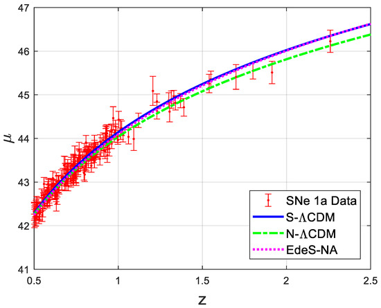
Figure 1. Data fit for $0.5<z<2.5$ based on models parameterized using $z<0.5$ data.

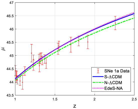
Figure 2. Data fit for $1.0<z<2.5$ based on models parameterized using $z<1.0$ data.

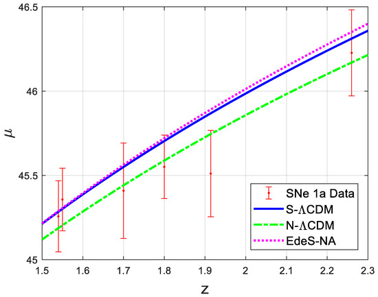
Figure 3. Data fit for $1.5<z<2.5$ based on models parameterized using $z<1.5$ data.

We present in Figure 4 the evolution of the density parameter ${\mathsf{\Omega }}_{\mathrm{\Lambda },z}$ corresponding the cosmological constant against the redshift $z$ evaluated using Equation (18). It increases from $0.16{\mathsf{\Omega }}_{\mathrm{\Lambda },0}$ at $z=\infty$ to ${\mathsf{\Omega }}_{\mathrm{\Lambda },0}=1$ at $z=0$. The figure shows the evolution over $0\le z\le 2.5$. In Figure 5 is shown the evolution of the equation of state parameter $w_{\mathrm{\Lambda },z}$ against $z$ using Equation (24) over the limited range of $0\le z\le 20$.

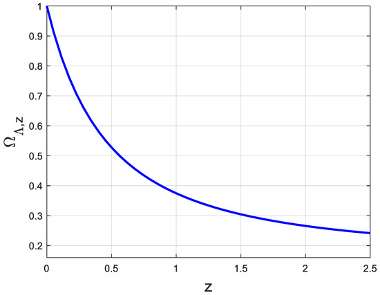
Figure 4. Density parameter ${\mathsf{\Omega }}_{\mathrm{\Lambda },z}$ vs. the redshift $z$.

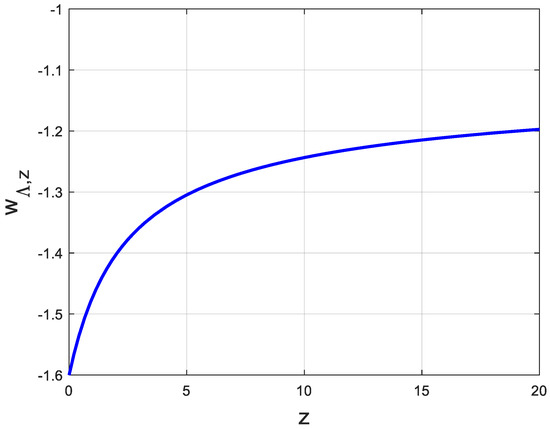
Figure 5. Equation of state parameter $w_{\mathrm{\Lambda },z}$ vs. redshift $z$.

4. Discussion

Referring to Table 2, let us first consider the columns corresponding to the dataset $z<0.5$. A marginally better parameterization for this data subset is achieved by N-$\mathrm{\Lambda }$CDM model as compared to the S-$\mathrm{\Lambda }$CDM model whereas EdeS-NA is significantly worse than the other two. However, the predictive data fit for the EdeS-NA model is significantly better than the other two models for data subsets $z>0.5$ and $z>1.0$, and significantly better than the S-$\mathrm{\Lambda }$CDM for the data subset $z>1.5$. In terms of the average probability, including the parameterization category, N-$\mathrm{\Lambda }$CDM model shines, whereas for the average of the predictive capability EdeS-NA model is marginally better than the N-$\mathrm{\Lambda }$CDM model and significantly better than the S-$\mathrm{\Lambda }$CDM model.

If we look at the next three columns in Table 2, corresponding to the model parameterization using the dataset $z<1.0$, our findings are as follows. The S-$\mathrm{\Lambda }$CDM model beats the other two in parameterization game, but predictive capability of the N-$\mathrm{\Lambda }$CDM model is unsurpassed by a good margin over the other two all through, including the average P% and the average predictive P%. The N-$\mathrm{\Lambda }$CDM performs even better when the model parameterization is done using dataset $z<1.5$ that is shown in the last three columns of Table 2.

The above is not surprising since N-$\mathrm{\Lambda }$CDM has $z$ dependent dark energy density. However, unlike the Chevallier-Polarski-Linder model, this redshift dependence does not require any additional fitting parameters; it is totally analytical and depends only on the assumption that the thermodynamic energy loss or gain of any volume of the universe is proportional to the energy in that volume.

Considering the fact that EdeS-NA model has no adjustable parameter other than the Hubble constant, the predictive fits offered by this model are surprising better than the S-$\mathrm{\Lambda }$CDM model when the models are parameterized with the most limited dataset.

Let us now focus on the trend in the model parameterizing categories in Table 1, i.e., the first row of categories. We notice that as we go from lower to higher $z$ datasets, the $R_0$ and ${\mathsf{\Omega }}_{m,0}$ values are increasing for the S-$\mathrm{\Lambda }$CDM model while these values are decreasing for N-$\mathrm{\Lambda }$CDM model. For EdeS-NA model $R_0$ is increasing too, but very little. Thus, the predictive P% has changed only very slightly for the Edes-NA model while the same has changed quite significantly for the other two models.

One could therefore infer that the N-$\mathrm{\Lambda }$CDM model is superior to the S-$\mathrm{\Lambda }$CDM in all respects studied in here. Even though EdeS-NA model is not the best for parameterizing the data, its predictive capabilities cannot be ignored, especially when models have only relatively low redshift data for parameterizing the models. Considering that EdeS-NA model is a single parameter model, whereas the other two models are two parameter models, Occam’s razor criterion would give EdeS-NA a very high rating. The application of these models to other cosmological phenomena without any bias would then determine critically the better model.

Having established from the analysis of the SNe Ia data that the superiority of N-$\mathrm{\Lambda }$CDM, and viability of EdeS-NA model, against the S-$\mathrm{\Lambda }$CDM model, we can have confidence in other finding of the model as well:

(a)

The nonadiabaticity of the universe when considered as dark energy density has redshift dependence proportional to ${\left(\frac{2}{5}+\frac{3}{5}{\left(1+z\right)}^{-\frac{3}{2}}\right)}^2$, Equation (18).

(b)

Similarly, the equation state parameter for matter can be considered to evolve as $\frac{2}{3}\ln \left(\frac{2}{5}+\frac{3}{5}{\left(1+z\right)}^{-\frac{3}{2}}\right)/\ln \left(1+z\right)$ Equation (23). Alternatively, the equation of state parameter for dark energy may be taken to be $w_{\mathrm{\Lambda },z}=-1+\frac{2}{3}\ln \left(\frac{2}{5}+\frac{3}{5}{\left(1+z\right)}^{-\frac{3}{2}}\right)/\ln \left(1+z\right)$, Equation (24).

(c)

All or a portion of the nonadiabadicity of the universe may be due to the variation of the gravitational constant $G$ and the speed of light $c$ through the relation $\frac{\dot{G}}{G}-\frac{2\dot{c}}{c}=1.8H_0=-\beta$, Equation (26). This, when combined with the LLR data analysis Equation (29), yields $\frac{\dot{G}}{G}=5.4H_0=-3\beta$ and $\frac{\dot{c}}{c}=1.8H_0=-\beta$ when we assume all the nonadiabadicity is vested in $\frac{\dot{G}}{G}$ and $\frac{\dot{c}}{c}$.

If we focus on the last finding (c), the challenge is to develop a method to measure the time dependence of $G$ and/or $c$ without assuming either of them to be constant. LLR method measures the round trip travel times of short laser pulses between observatories on the Earth and retroreflectors on the Moon. So, the distance measurement depends on the constancy of the speed of light. However, since $G$ and $c$ both enter the Friedmann equation, we cannot treat one to be dynamic without giving the same status to the other. We should therefore use their time dependent forms $G=G_0{e}^{3\beta \left(t_0-t\right)}$ and $c=c_0{e}^{\beta \left(t_0-t\right)}$ when time dependency of $G$ and $c$ could impact the measurements outcome. The value of the nonadiabaticity parameter $\beta$ may be taken as $-1.8H_0$ until a better value is determined.

The concern about the use of a dimensionful constant in this paper may be dispelled by knowing that one could arrange to rewrite, for example $\frac{\dot{c}}{c}=1.8H_0$, $\frac{\dot{G}}{G}=5.4H_0$, $c=c_0{e}^{\beta \left(t_0-t\right)}$ and $G=G_0{e}^{3\beta \left(t_0-t\right)}$, in their dimensionless forms as $\frac{\dot{c}}{c{H}_0}=1.8$, $\frac{\dot{G}}{G{H}_0}=5.4$, $c/c_0=e^{\beta \left(t_0-t\right)}$ and $G/G_0=e^{3\beta \left(t_0-t\right)}$, respectively. But this does not alter the findings presented in here. Thus, one could show the variability of the constants expressed in terms of their present value denoted by adding subscript 0 to it.

5. Conclusions

The nonadiabatic foundation of the universe, that takes into account in its thermodynamics the loss or gain of the energy of the universe in any volume to be proportional to the energy in the volume, has been shown to be the basis of a new $\mathrm{\Lambda }$CDM cosmological model that not only fits the best SNe Ia data well, but has the predictive capability that is superior to the standard $\mathrm{\Lambda }$CDM model. The new nonadiabatic foundation also provides parameter free analytical expressions for the redshift (i.e., time) dependence of dark energy and equation state parameters, and the possible time evolution of the gravitational constant and the speed of light.

References

- COSINE-100 Collaboration. An experiment to search for dark-matter interactions using sodium iodide detectors. Nature 2018, 564, 83–86. [Google Scholar] [CrossRef] [PubMed]
- Bernabei, R.; Belli, P.; Bussolotti, A.; Cappella, F.; Caracciolo, V.; Cerulli, R.; Dai, C.J.; d’Angelo, A.; Di Marco, A.; He, H.L.; et al. First model independent results from DAMA/LIBRA-phase2. arXiv 2018, arXiv:1805.10486. Available online: https://arxiv.org/abs/1805.10486 (accessed on 25 June 2019).
- Farnes, J.S. A unifying theory of dark energy and dark matter: Negative masses and matter creation within a modified ΛCDM framework. Astron. Astrophys. 2018, 620, A92. [Google Scholar] [CrossRef]
- Weyl, H. Eine neue Erweiterung der Relativistätstheorie. Annalen der Physik 1919, 59, 129. [Google Scholar]
- Eddington, A.S. New Pathways in Science; Cambridge University Press: Cambridge, UK, 1934. [Google Scholar]
- Dirac, P.A.M. The cosmological constants. Nature 1937, 139, 323. [Google Scholar] [CrossRef]
- Brans, C.; Dicke, R.H. Mach’s principle and a relativistic theory of gravitation. Phys. Rev. 1961, 124, 925–935. [Google Scholar] [CrossRef]
- Einstein, A. Über das Relativitätsprinzip und die aus demselben gezogenen Folgerungen. Jahrbuch fur Radioaktivitat und Elektronik 1907, 4, 411–462. [Google Scholar]
- Dicke, R.H. Gravitation without a principle of equivalence. Rev. Mod. Phys. 1957, 29, 363. [Google Scholar] [CrossRef]
- Petit, J.P. An interpretation of cosmological model with variable light velocity. Mod. Phys. Lett. 1988, A3, 1527–1532. [Google Scholar] [CrossRef]
- Moffat, J.W. Superluminary universe: A possible solution to the initial value problem in cosmology. Int. J. Mod. Phys. 1993, D2, 351. [Google Scholar] [CrossRef]
- Salzano, V.; Dabrowski, M.P. Statistical hierarchy of varying speed of light theories. Astrophys. J. 2017, 851, 97. [Google Scholar] [CrossRef]
- Duff, M. Comment on time-variation of fundamental constants. arXiv 2016, arXiv:Hep-th/0208093 v4. Available online: https://arxiv.org/abs/hep-th/0208093 (accessed on 25 June 2019).
- Ellis, G.F.R.; Uzan, J.P. ‘c’ is the speed of light, isn’t it? Am. J. Phys. 2005, 73, 240–253. [Google Scholar] [CrossRef]
- Uzan, J.-P. The fundamental constants and their variation: Observational status and theoretical motivation. Rev. Mod. Phys. 2003, 75, 403. [Google Scholar] [CrossRef]
- Uzan, J.P. Varying constants, gravitation and cosmology. Living Rev. Relativ. 2011, 14, 2. [Google Scholar] [CrossRef] [PubMed]
- Duff, M.J. How fundamental are fundamental constants? arXiv 2014, arXiv:1412.2040. Available online: https://arxiv.org/abs/1412.2040 (accessed on 25 June 2019).
- Chiba, T. Constancy of the constants of nature: Updates. Prog. Phys. 2011, 126, 993–1019. [Google Scholar] [CrossRef]
- Martins, C.J.A.P. The status of varying constants: A review of physics, searches and implications. Rep. Prog. Phys. 2017, 80, 126902. [Google Scholar] [CrossRef] [PubMed]
- Magueijo, J. New varying speed of light theories. Rep. Prog. Phys. 2003, 66, 2025. [Google Scholar] [CrossRef]
- Gupta, R.P. Varying physical constants, astrometric anomalies, redshift and Hubble units. Galaxies 2019, 7, 55. [Google Scholar] [CrossRef]
- Gupta, R.P. SNe Ia redshift in a nonadiabatic universe. Universe 2018, 4, 104. [Google Scholar] [CrossRef]
- Chevallier, M.; Polarski, D. Accelerating universe with scaling dark matter. Int. J. Mod. Phys. 2001, D10, 213–223. [Google Scholar] [CrossRef]
- Linder, E.V. Exploring the expansion history of the universe. Phys. Rev. Lett. 2003, 90, 091301. [Google Scholar] [CrossRef] [PubMed]
- Scolnic, D.M.; Jones, D.O.; Rest, A.; Pan, Y.C.; Chornock, R.; Foley, R.J.; Huber, M.E.; Kessler, R.; Narayan, G.; Riess, A.G.; et al. The complete light curve sample of spectroscopically confirmed SNe Ia from Pan-STARRS1 and cosmological constraints from the combined pantheon samzple. Astrophys. J. 2018, 859, 101, data file taken from: Catalogs of Cosmologically Useful Type Ia Supernovae from Pan-STARRS (“PS1COSMO”). Available online: https://archive.stsci.edu/hlsps/ps1cosmo/scolnic/hlsp_ps1cosmo_panstarrs_gpc1_all_model_v1_lcparam-full.txt (accessed on 11 December 2018).
- Ryden, B. Introduction to Cosmology; Cambridge University Press: Cambridge, UK, 2017. [Google Scholar]
- Aviles, A.; Gruber, C.; Luongo, O.; Quevedo, H. Cosmography and constraints of the equation of state of the universe in various parametrization. Phys. Rev. D 2012, 86, 123516. [Google Scholar] [CrossRef]
- Capozziello, S.; De Laurentis, M.; Luongo, O.; Ruggeri, A.C. Cosmographic constraints and cosmic fluids. Galaxies 2013, 1, 216–260. [Google Scholar] [CrossRef]
- Gruber, C.; Luongo, D. Cosmographic analysis of the equation of state of the universe through Padé approximations. Phys. Rev. D 2014, 89, 103506. [Google Scholar] [CrossRef]
- Dunsby, P.K.S.; Luongo, O. On the theory and application of modern cosmography. Int. J. Geom. Meth. Mod. Phys. 2016, 13, 1630002. [Google Scholar] [CrossRef]
- Capoziello, S.; D’Agostino, R.; Luongo, O. Cosmographic Analysis with Chebyshev polynomials. Mon. Not. Roy. Astron. Soc. 2018, 476, 3924–3938. [Google Scholar] [CrossRef]
- Aviles, A.; Bravetti, A.; Capozziello, S.; Luongo, O. Precision cosmology with Padé rational approximations: Theoretical predictions versus observational limits. Phys. Rev. D 2014, 90, 043531. [Google Scholar] [CrossRef]
- Gupta, R.P. Static and dynamic components of the redshift. Int. J. Astron. Astrophys. 2018, 8, 219–229. [Google Scholar] [CrossRef]
- Hofmann, F.; Müller, J. Relativistic tests with lunar laser ranging. Class. Quant. Grav. 2018, 35, 035015. [Google Scholar] [CrossRef]
- Merkowitz, S.M. Test of gravity using lunar laser ranging. Living. Rev. Rel. 2010, 13, 7. [Google Scholar] [CrossRef]
- Gupta, R.P. Weighing Cosmological Models with SNe Ia and Gamma Ray Burst Redshift Data. Universe 2019, 5, 102. [Google Scholar] [CrossRef]
- Walker, J. Chi-Square Calculator. 2019. Available online: https://www.fourmilab.ch/rpkp/experiments/analysis/chiCalc.html (accessed on 25 June 2019).
- Vishwakarma, R.G.; Narlikar, J.V. Is it no longer necessary to test cosmologies with type 1a supernovae? Universe 2018, 4, 73. [Google Scholar] [CrossRef]
© 2019 by the author. Licensee MDPI, Basel, Switzerland. This article is an open access article distributed under the terms and conditions of the Creative Commons Attribution (CC BY) license (http://creativecommons.org/licenses/by/4.0/).