Fractional Variability—A Tool to Study Blazar Variability

Abstract

Active Galactic Nuclei emit radiation over the whole electromagnetic spectrum up to TeV energies. Blazars are one subtype with their jets pointing towards the observer. One of their typical features is extreme variability on timescales, from minutes to years. The fractional variability is an often used parameter for investigating the degree of variability of a light curve. Different detection methods and sensitivities of the instruments result in differently binned data and light curves with gaps. As they can influence the physics interpretation of the broadband variability, the effects of these differences on the fractional variability need to be studied. In this paper, we study the systematic effects of completeness in time coverage and the sampling rate. Using public data from instruments monitoring blazars in various energy ranges, we study the variability of the bright TeV blazars Mrk 421 and Mrk 501 over the electromagnetic spectrum, taking into account the systematic effects, and compare our findings with previous results. Especially in the TeV range, the fractional variability is higher than in previous studies, which can be explained by the much longer (seven years compared to few weeks) and more complete data sample.

1. Blazar Variability

Blazars are a subclass of active galactic nuclei (AGN), which are radio-loud and have one of the relativistic jets pointing in a small angle to the line of sight of the observers. A typical feature of blazars is a variable flux showing changes on time ranges from minutes to years. One prominent source for variability over the complete electromagnetic spectrum is the blazar Mrk 421. This source was first observed in the year 1992 at TeV energies and was the first extragalactic source detected in this energy range [1]. It is one of the most observed TeV sources in the sky. Another frequently observed source in the TeV energy range is Mrk 501. This source is known as a highly variable source since its discovery in very high energy gamma rays in the year 1996 [2].

The spectral energy distributions (SEDs) of the blazars Mrk 421 and Mrk 501 are shown in Figure 1. The SEDs have the typical two-bump structure, with synchrotron radiation of the relativistic electrons in the jet responsible for the low energy bump. The underlying processes of the high energetic bump are different and still highly debated. There are several models for the gamma-ray emission at high energies. The different emission models can be tested by using contemporaneous multi-wavelength data. The correlation between the different energies and the duration of flares are two important parameters for this.

In this context, we want to study the degree of variability in the different energy bands. Of course, the degree of variability depends also on the exact position of the two peaks in the SED, and a peak shift can influence the result.

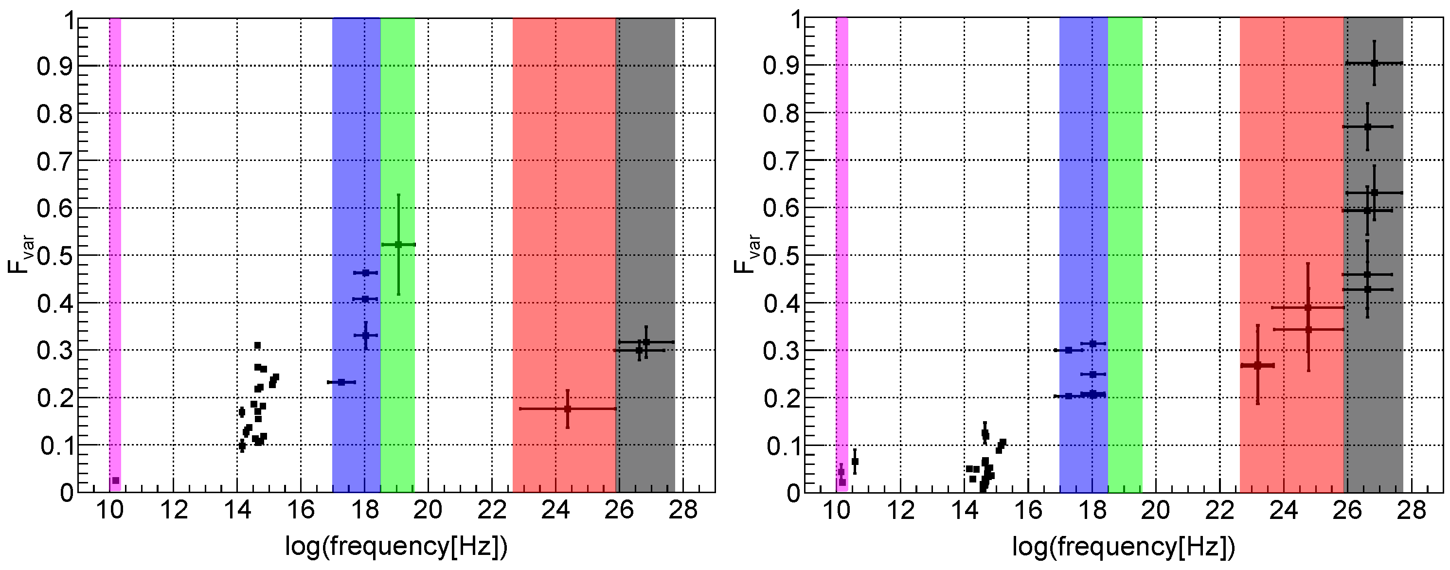
2. Fractional Variability

To quantify the intensity of the variability in a given sample of N data points $x_i$ the variance $S^2$$={(N-1)}^{-1}{\sum }_{i=1}^N{(\langle x\rangle -x_i)}^2$ can be used. In the case of blazar light curves, this sample is the light curve, which includes measurement uncertainties ${\sigma }_{err,i}$. To take these uncertainties into account, the fractional variability is often the parameter of choice. It combines the variance of the data points and includes the additional variance that arises from the measuring of these uncertainties. This so-called fractional excess variance or normalized excess variance is given in [5] as

$$\begin{array}{c}\hfill {\sigma }_{\mathrm{NXS}}^2=\frac{S^2-\langle {\sigma }_{err}^2\rangle }{{\langle x\rangle }^2},\end{array}$$

(1)

where $\langle {\sigma }_{err}^2\rangle$ is the mean square error defined as

$$\begin{array}{c}\hfill \langle {\sigma }_{err}^2\rangle =\frac{1}{N}\sum _{i=1}^N{\sigma }_{err,i}^2.\end{array}$$

(2)

The square root of the fractional excess variance ${\sigma }_{\mathrm{NXS}}^2$ is the so-called fractional variability

$$\begin{array}{c}\hfill F_{\mathrm{var}}=\sqrt{\frac{S^2-\langle {\sigma }_{err}^2\rangle }{{\langle x\rangle }^2}}.\end{array}$$

(3)

This parameter contains exactly the same information as the normalized excess variance. The uncertainty of $F_{\mathrm{var}}$ according to [6] is given by

$$\begin{array}{c}\hfill \Delta F_{\mathrm{var}}=\sqrt{F_{\mathrm{var}}^2+err\left({\sigma }_{\mathrm{NXS}}^2\right)}-F_{\mathrm{var}}\end{array}$$

(4)

with the uncertainty of the normalized excess variance (taken from [7])

$$\begin{array}{c}\hfill err\left({\sigma }_{\mathrm{NXS}}^2\right)=\sqrt{\left(\sqrt{\frac{2}{N}}\frac{\langle {\sigma }_{err}^2\rangle }{{\langle x\rangle }^2}\right)+{\left(\sqrt{\frac{\langle {\sigma }_{err}^2\rangle }{N}}\frac{2F_{\mathrm{var}}}{\langle x\rangle }\right)}^2}.\end{array}$$

(5)

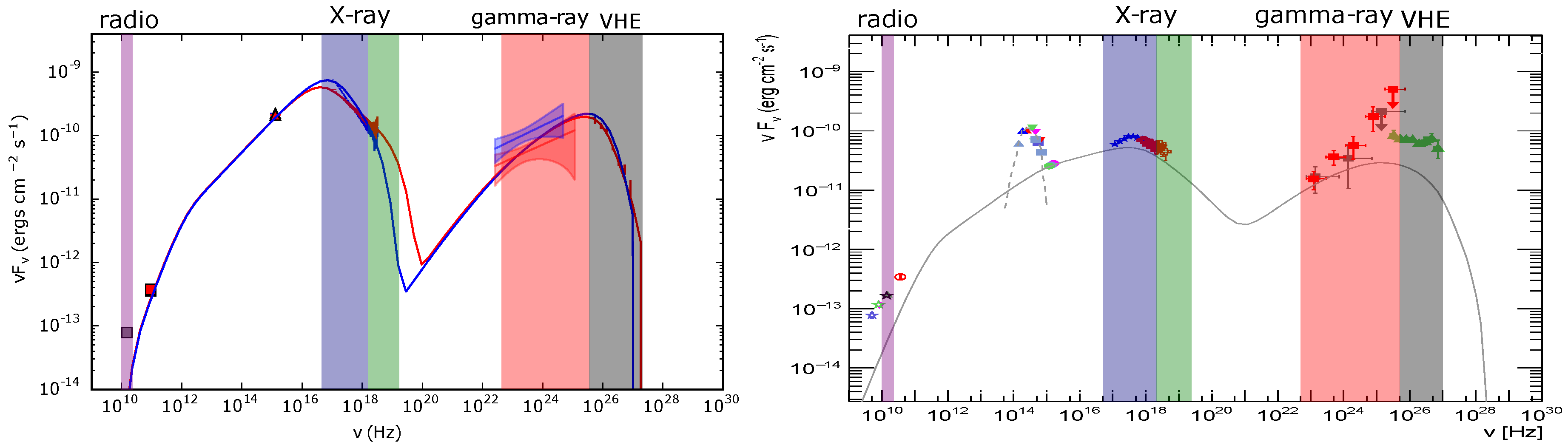
3. Multi-Wavelength View of the Fractional Variability

To quantity the variability of a source, in many studies $F_{\mathrm{var}}$ is given. The blazars Mrk 421 and Mrk 501 have often been observed in multi-wavelength campaigns [8]. Some former variability studies of Mrk 421 can be found in [3,9,10,11,12,13]. Examples for Mrk 501 studies are [4,14,15,16,17]. The studies cover a time range beginning with data from March 2001 for Mrk 421 and with May 2005 for Mrk 501. In the early years, there are bigger gaps in the light curves than the current ones, and also the energy ranges covered by the observations were smaller. Since 2009, systematic MWL campaigns have been organized containing data from radio to TeV energies [8]. A limitation of these studies is that the data samples are often short or the gaps in the data sample are large. Only the all-sky monitoring instruments can provide continuous data.

To compare $F_{\mathrm{var}}$ of different wavelength, it is crucial to use data of the same time window and with a time binning of at least the expected and studied time range for the variabilities. Limited by the data samples of nonmonitoring instruments, MWL studies of the fractional variability so far take into account limited data samples of the duration of single days (e.g., [3]) to 2.3 years ([11]). Figure 2 shows a comparison of $F_{\mathrm{var}}$ vs. frequency for Mrk 421 and Mrk 501. The major difference is that for Mrk 421, the maximum of the variability is in the X-ray regime, while for Mrk 501 the maximum is at VHE energies. This difference is often seen, and it is indicating that this is a hint of different particle population, environment, and/or processes in the jets [10]. However, there are also studies measuring the maximum $F_{\mathrm{var}}$ at VHE ([3,11]). The shape of the $F_{\mathrm{var}}$ vs. energy plot of Mrk 421 is an increase up to X-rays, than a drop down and an increase again up to VHE. This structure looks like a double hump, which was not seen for Mrk 501 in the past, because there one can see a steady increase of the variability. In [17], they report a double peak shape also for Mrk 501, so it looks like the structure of the $F_{\mathrm{var}}$ vs. energy plot is not a characteristic of a source. Based on the results so far, the shape of the plot seems to be changing with time. Since there is no uniform shape of the $F_{\mathrm{var}}$ vs. energy plot, a systematic study is necessary to figure out what causes the differences.

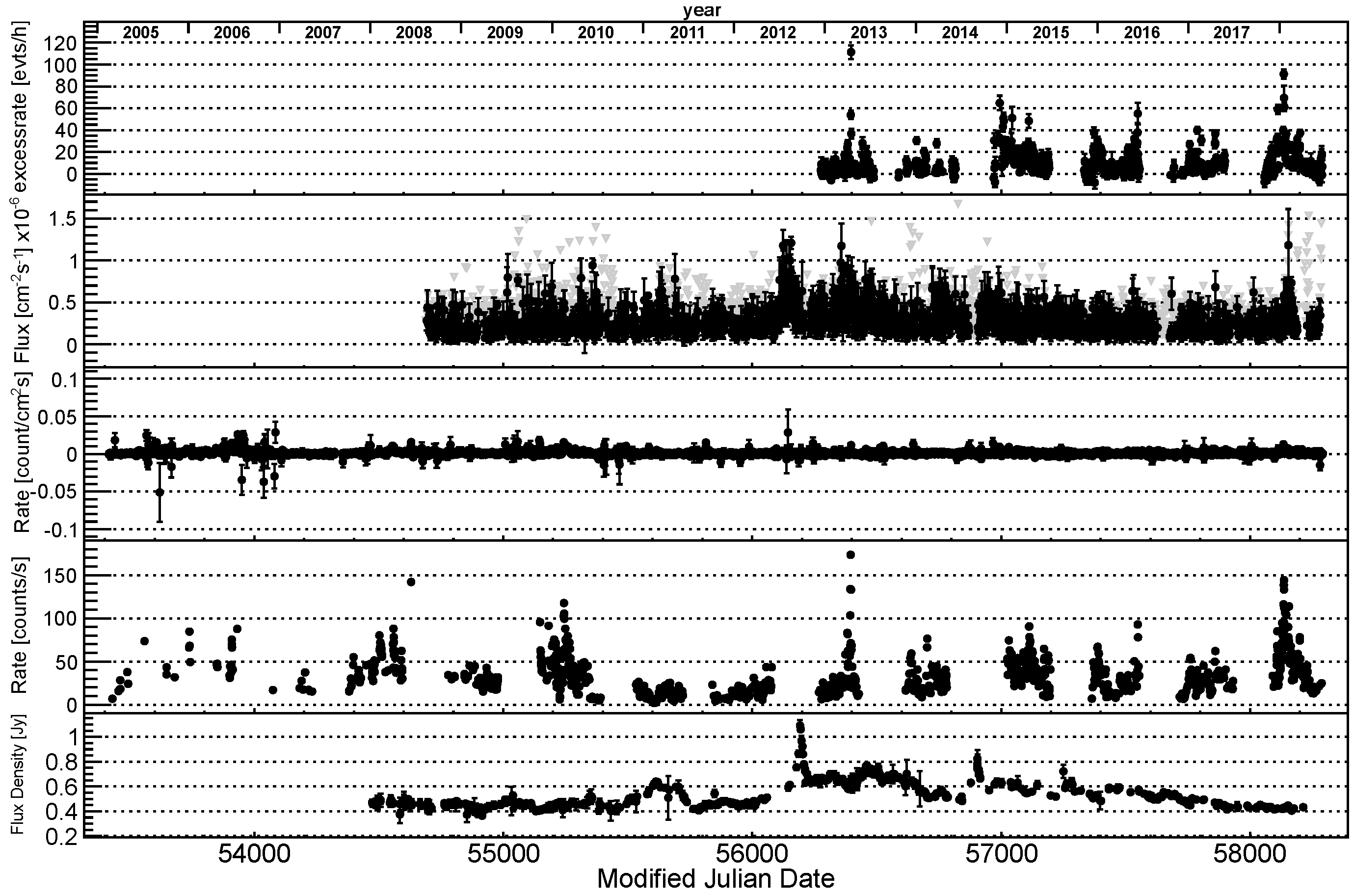
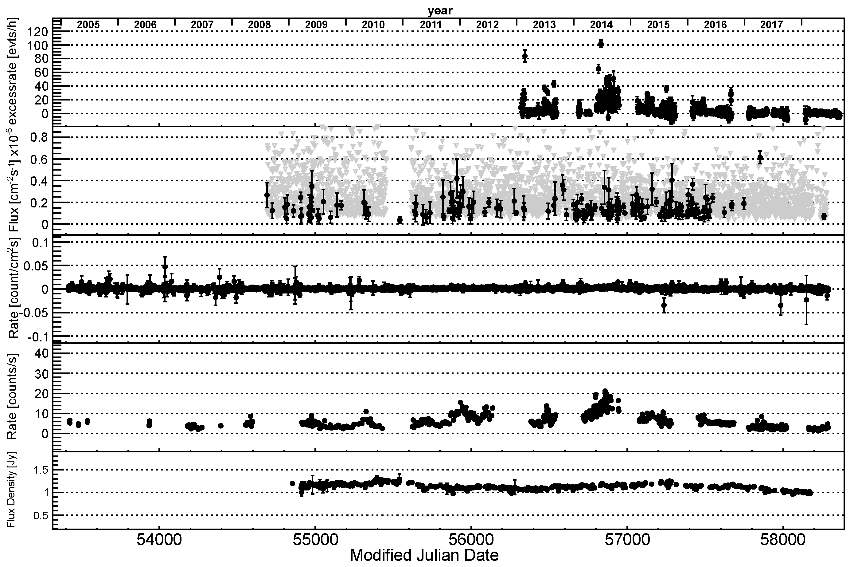
4. Data Sample

To characterize the variability of a source, an unbiased data sample is necessary to catch all variations in the activity of a source, not only in high flux states, but also in low flux states. Therefore, monitoring programs in all spectral bands are crucial. To compare the variability of a source over the different energy ranges, simultaneous data are needed. For our samples we used radio, X-ray, and gamma-ray data. The energy ranges are marked in the SEDs of Figure 1. It is also planned to include optical data in a future study.

Radio data are from the Owens Valley Radio Observatory (OVRO). It is a 40 m telescope that observes at 15 GHz. It is used for a monitoring program following the blazars observed with Fermi. This results in about two observations per week and source [18]. These public data1 are available labeled as daily binning, but for comparison with the other instruments and measurements it should be mentioned that the observations are short (order of seconds to minutes) and not in a daily cadence.

X-ray observations have been carried out with the Swift satellite since 2004. Public data are available from the following instruments on board of the Swift satellite: The X-Ray Telescope (XRT) with an energy range of 0.2 keV up to 10 keV and the Burst Alert Telescope (BAT) with an energy range of 15 keV up to 150 keV. BAT light curves are available in daily binning and orbit wise binning2 [19]. BAT provides a very complete data sample, because with a field of view of 1.4 steradians, it monitors the whole sky orbitwise. The coverage of a typical sky point is about 4 h per day. The XRT count rate curves are available in daily binning3 [20], but have gaps, because the instrument does pointed observations, and therefore not every days data from each source are available.

We use gamma-ray data from the Fermi Gamma-ray Space Telescope. The Large Area Telescope (LAT) of the satellite is scanning the whole sky, and therefore it is a perfect instrument for systematic long-term studies [21]. Public light curves are available in weekly and daily binning4${}^{,}$5. On some days, the flux state of the source only allows to calculate an upper limit. These upper limits are not taken into account for the fractional variability calculations. Fermi LAT covers an energy range of 100 MeV up to 300 GeV. The coverage of a sky point is about 30 min every second orbit. The orbital period is about 96 min. This results in 2 h coverage per day.

The First G-APD Cherenkov Telescope (FACT) provides data in the very high energy (VHE) range. FACT monitors the brightest TeV sources in the sky. Being a ground based instrument, the sources are not visible 24 h per day, causing gaps in the light curves. As the observations are limited to night time, seasonal gaps are introduced to the light curves. Additional gaps are caused by bad weather and other environmental influences. Public data are available in daily binning and in 20 min binning6 [22].

The multi-wavelength light curve of Mrk 421 from the instruments used is shown in Figure 3 and for Mrk 501 in Figure 4. The used data are binned daily, and the maximum available time range is shown.

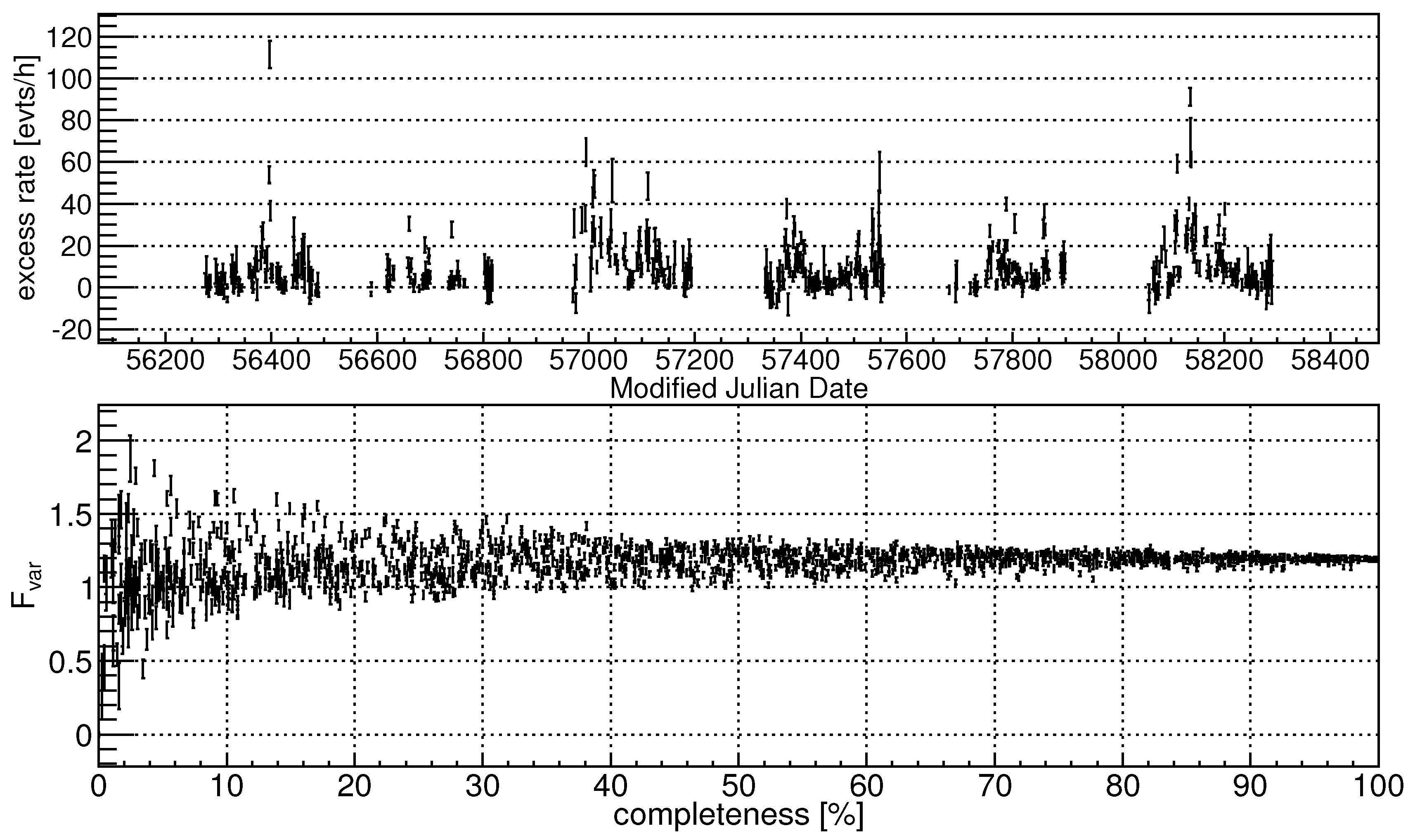
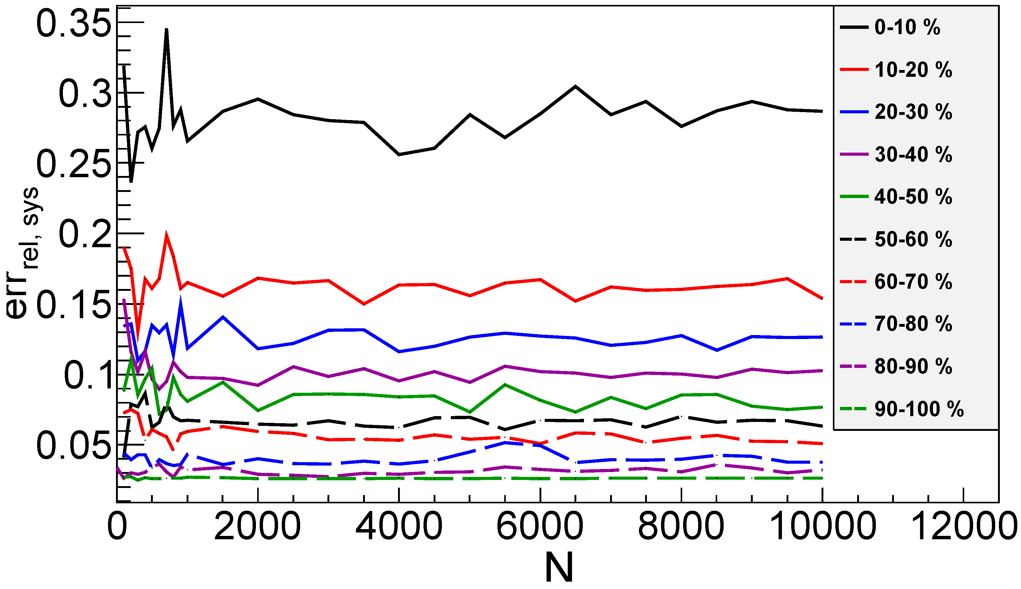
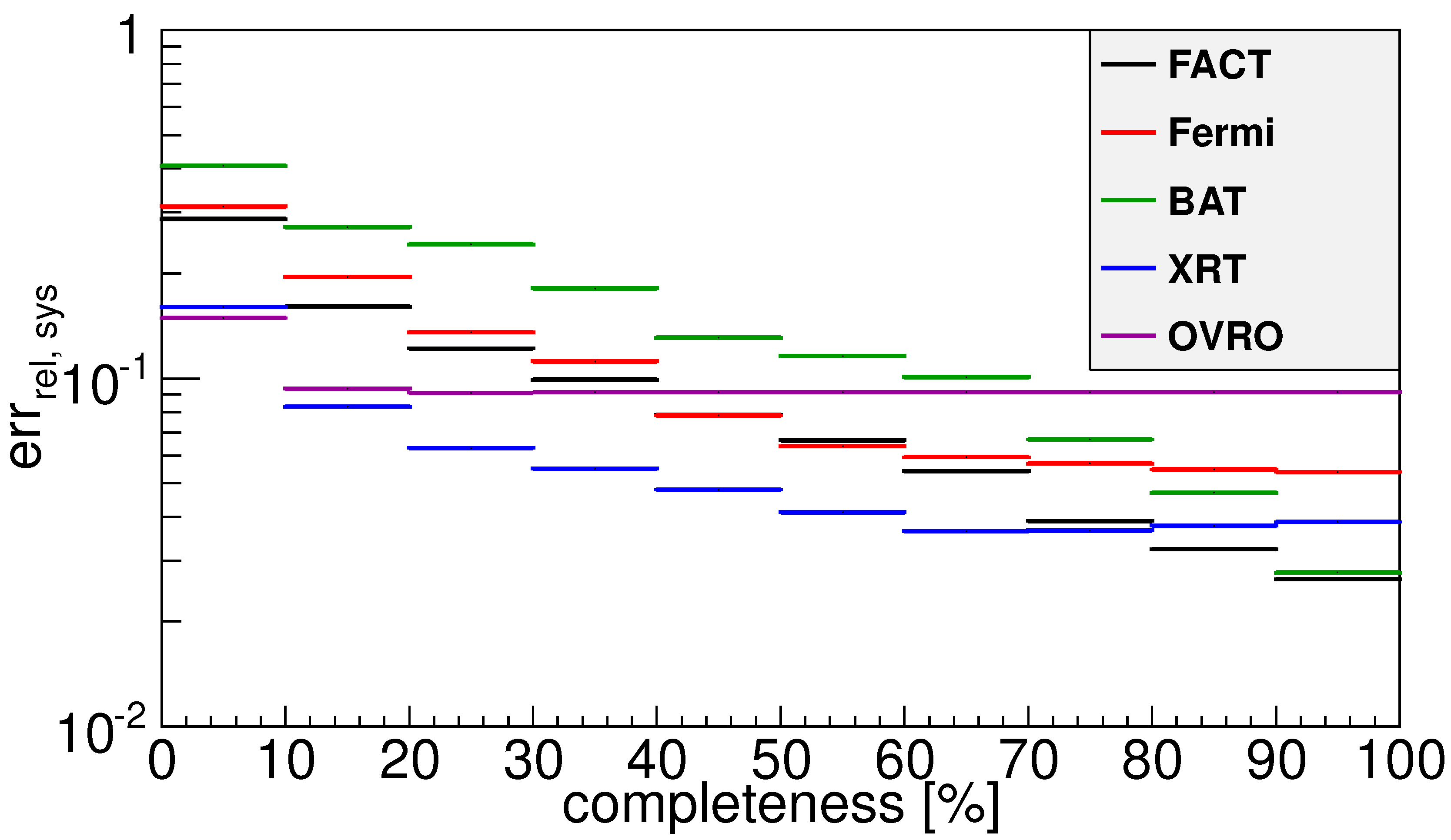
5. Systematic Study

The fractional variability itself does not use any timing information of the light curve, because of this, it is necessary to be very careful in choosing the data sample and interpreting the result. The studied time scale of the variability is limited by the time binning and cadence of the data sample. Another important point is that gaps in the sample have an impact on the outcome of a variability study, and for comparing data from different instruments only simultaneous data can be easily interpreted. As fast variability on time scales from minutes to hours has been seen in blazars [23,24], this means that nonsimultaneous data could result in light curves lacking flaring activities in one band and therefore different results in Fvar, which would naturally have a larger impact in smaller data samples.

It is important to understand how the fractional variability changes with the characteristics of the data sample, and which uncertainties can be expected, if a data sample is incomplete.

5.1. Completeness of Data Sample

Depending on the observing strategies and the observing methods, completely continuous monitoring is very challenging, and most data samples show gaps on different time scales. Also the sampling rate and time, based on the expected variability time scale can be a reason for a low cadence, and therefore gaps in a light curve. For example, typical variations in the radio band have a time scale of at least a few days. Therefore OVRO observe this blazars every few days for about a minute. The question is how the outcome of a variability calculation changes when using an incomplete data sample. Effects on the fractional variability are studied here with the multi-wavelength data sample of Mrk 421.

For the first part of the study, we define the existing data sample as 100% completeness. To simulate an incomplete data sample, we randomly remove data points. As an example, the FACT data are shown in Figure 5. The upper panel shows the complete light curve. From this, between 0% and 100% of the data points are removed, and the fractional variability is calculated, resulting in one point in the lower panel of Figure 5. This procedure is repeated N times, resulting in the distribution in the lower panel of Figure 5. As expected, the spread of the fractional variability increases with the fraction of removed data.

To evaluate how large N has to be, i.e., how often the procedure needs to be repeated, we study the relative uncertainty versus N. For this, we calculate the 16% and 84% quantile for each 10% bin in Figure 5 and plot the relative value with respect to N (see Figure 6). For small N, the 16% and 84% quantiles fluctuate as expected; but for large N (N > 6000), the relative uncertainty converges. For the further steps in the study, we use the relative uncertainty calculated with N = 10,000.

This procedure is repeated for every data sample of the different instruments in order to calculate the systematic uncertainty introduced by an incomplete multi-wavelength data sample. The result is shown in Figure 7. Like expected, there is a systematic error when using an incomplete data sample. This error decreases with the completeness of the data sample.

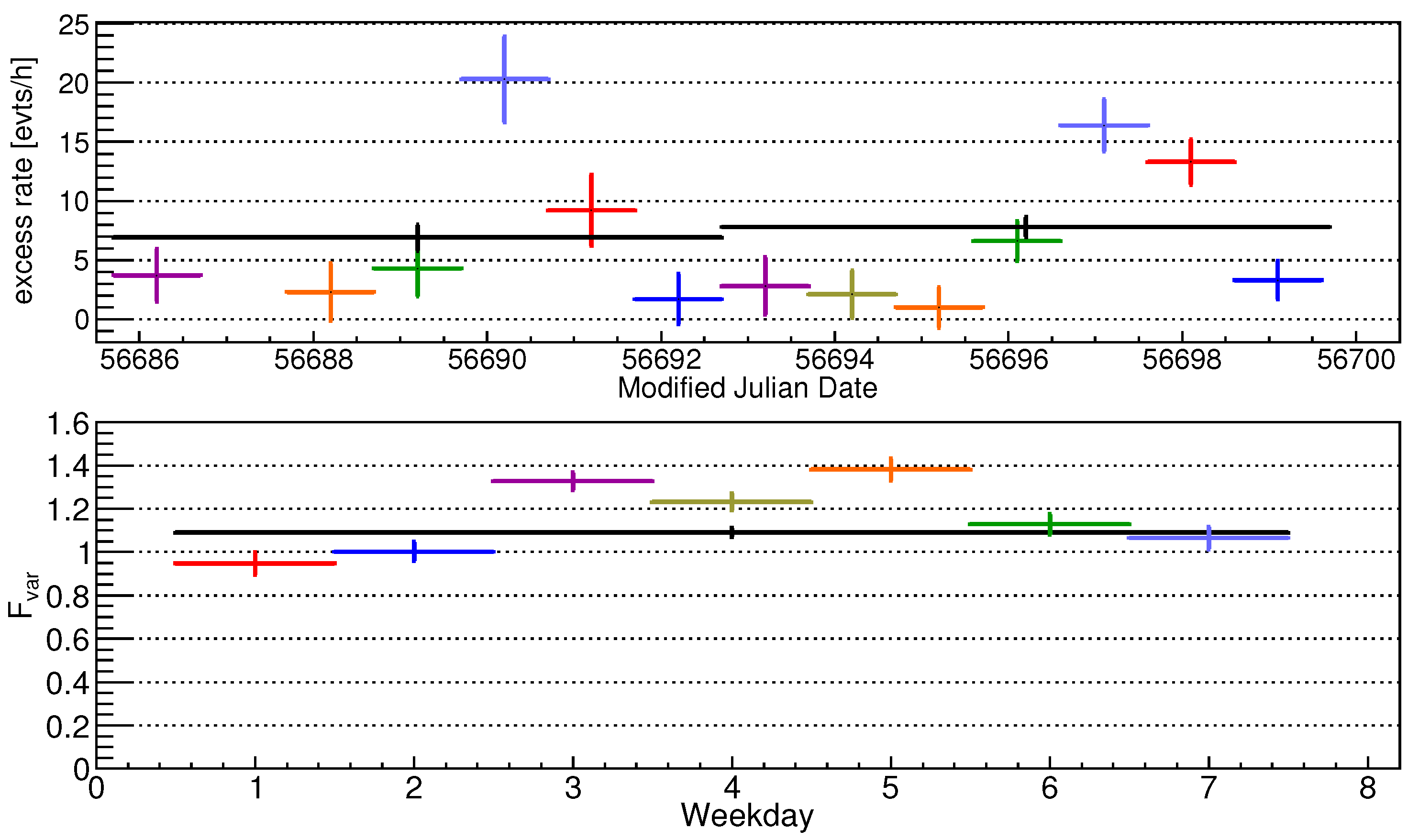
5.2. Gaps vs. Averaging

While some data samples have gaps on longer time scales, e.g., limited sampling in case of XRT, others have gaps on short time scales, e.g., the effect of orbits in Fermi. To account for the limited detector sensitivity, data have to be grouped in larger bins and an average flux is calculated. To assess the effect of such different strategies (short very sensitive observations vs. almost continuous low-sensitivity monitoring), we compare the fractional of weekly binning with week–day binning. For the latter, we calculate the fractional variability using daily binning, but only the data points of one day of the week, e.g., Friday. This study is done with data of Mrk 421 for both FACT and Fermi LAT. The results are shown in Figure 8 and Figure 9.

The upper plot of Figure 8 shows a zoom on the FACT light curve of two weeks. The different colors indicate the individual weekdays and the black points show the weekly binned excess rate. The lower plot compares the fractional variability of each weekday with the weekly fractional variability. One can see that the value of the fractional variability would vary by 27%, if only one observation per week was available. Still, the values of the individual days scatter around the weekly value.

For the Fermi LAT data, the result is different than for the FACT data, because the Fermi LAT daily light curve of Mrk 421 contains a lot of upper limits, which are not taken into account for the calculation of the fractional variability. For the weekly binning, the data of every day are used for one week bin and not ignored like in the case of a upper limit. The fractional variability of one weekday is smaller than when using the weekly bins. An upper limit is always associated with a flux that is lower than the sensitivity of the instrument. Therefore, the lowest fluxes of the source are missing in such a data sample and the full flux range of the source is not entering the variability study.

5.3. Further Effects

There are some more characteristics of a data sample that can have a systematic effect on the outcome of the calculation of the fractional variability. The influences of the duration of the data points and the cadence of data taking are planned to be investigated in future.

6. Results

The multi-wavelength data of Mrk 421 and Mrk 501 (Figure 3 and Figure 4) are daily binned, but with a variety of gaps making the data sample incomplete. A variability study has a systematic uncertainty caused by this incompleteness.

6.1. Mrk 421

In Figure 10 (upper plot), the complete time range of FACT data (December 2012–June 2018), is used for a multi-wavelength comparison of the fractional variability of Mrk 421. This is the first time a 6 year long MWL-data sample is used to calculate $F_{\mathrm{var}}$. The black error bars are the standard errors (Equation (4)) and the gray boxes are the systematic uncertainties due to the incomplete data sample. The completeness of the data sets are 34% (FACT), 53% (Fermi), 97% (BAT), 28% (XRT), and 16% (OVRO). For the satellites, the coverage in the orbits is not taken into account in this calculation, as the studied time scale here is days, not minutes to hours. One can see that the systematic uncertainty can be much larger than the standard error and needs to be taken into account. For example, due to the seasonal gaps of FACT observations, when the source is not visible during night time there is a significant lack of information, which causes this uncertainty. In addition, the larger degree of variability introduces larger systematic uncertainties as it is defined as a relative value here.

The study of only one observing season is shown in Figure 10 (lower plot). In 2013, the fractional variability is significantly higher than in the 6-year period. This might be caused by the huge flare on 14 April 2013 and the associated activity. The completeness of the seasonal data sets are 55% (FACT), 68% (Fermi), 98% (BAT), 36% (XRT), and 60% (OVRO).

One can see in both plots the double hump structure that the historical results have shown. A major difference between the historical studies and this one is the value of the fractional variability. The value is larger for this long time period compared to the studies in the past (e.g., [10]). In the historical study shown in Figure 2, $F_{\mathrm{var}}$ is around 0.03 for radio, between 0.2 and 0.6 for X-ray, around 0.15 for gamma-ray, and around 0.3 for VHE gamma-ray data. The calculated fractional variabilities for the complete time range and the 2013 season can be found in

Table 1. Results of the variability study of Mrk 421 (see Figure 10) for the FACT time range, and the 2013 observing season of FACT and Mrk 501 (see Figure 11) for the FACT time range.

Mrk421	${\mathit{F}}_{\mathit{var},\mathit{FACT}}$	${\mathit{F}}_{\mathit{var},\mathit{Fermi}}$	${\mathit{F}}_{\mathit{var},\mathit{BAT}}$	${\mathit{F}}_{\mathit{var},\mathit{XRT}}$	${\mathit{F}}_{\mathit{var},\mathit{OVRO}}$
complete time range	$1.19\pm 0.13$	$0.289\pm 0.031$	$0.939\pm 0.068$	$0.647\pm 0.041$	$0.155\pm 0.017$
2013 observing season	$1.84\pm 0.17$	$0.256\pm 0.043$	$1.25\pm 0.14$	$0.955\pm 0.053$	$0.0630\pm 0.0087$
Mrk501	${\mathit{F}}_{\mathit{var},\mathit{FACT}}$	${\mathit{F}}_{\mathit{var},\mathit{Fermi}}$	${\mathit{F}}_{\mathit{var},\mathit{BAT}}$	${\mathit{F}}_{\mathit{var},\mathit{XRT}}$	${\mathit{F}}_{\mathit{var},\mathit{OVRO}}$
complete time range	$1.70\pm 0.16$	$0.36\pm 0.14$	$0.279\pm 0.076$	$0.610\pm 0.040$	$0.0466\pm 0.0057$

. This confirms that the variability of a blazar is not described comprehensively with a short-term multi-wavelength study, and long term monitoring is needed.

6.2. Mrk 501

The $F_{\mathrm{var}}$ vs. energy plot of Mrk 501 for the FACT time range (January 2013–June 2018) is shown in Figure 11. Also, the systematic errors caused by gaps in the light curve are drawn as gray boxes. The completeness of the data sets for the FACT time range are 40% (FACT), 7% (Fermi), 97% (BAT), 21% (XRT), and 11% (OVRO). The calculated fractional variabilities of Mrk 501 can be found in Table 1. Here, one can also see a double hump structure, but the first maximum of the peak is at a lower energy. For Mrk 421, the maximum of the low energy peak is in the BAT energy range (15 keV to 150 keV) or above, while for Mrk 501 the peak is in the XRT range (0.2 keV to 10 keV) and the fractional variability drops for the BAT data. Some historical variability studies claimed this structure as a difference between Mrk 421 and Mrk 501. Also for Mrk 501, the fractional variability is higher at the low energy peak and in the VHE regime than in previous studies (e.g., [4]). In the shown historical study (blue points), $F_{\mathrm{var}}$ ranges from 0.2 to 0.4 for the X-ray data and from 0.4 to 0.9 for VHE data; while for the complete data sample the values range from 0.2 to 0.6 in the X-ray data and reaches 1.7 in the VHE data.

From this comparison, it seems that the shape of the $F_{\mathrm{var}}$ vs. energy curve is dependent on the chosen time range of the study. Now, it is important to understand how the shape of this curve correlates with time changing properties of a source, for example the flux state of the source.

7. Summary and Discussion

To compare the variability of a source for different energy ranges or different time ranges, the fractional variability is a useful tool. In the past, it has been used for many MWL studies. However, in most studies systematic effects are not taken into account. The detection methods are changing along the electromagnetic spectrum. Also, the observing strategy depends on the instrument. This leads to data samples with major differences. The characteristics of the data samples can influence the result of a variability study, so a systematic study of these effects is needed. We used daily-binned long-term data samples from different instruments, from radio up to TeV energies. Due to weather, technical problems, or observing strategy, the light curves contain gaps. To take the completeness of the data sample into account, a systematic error was introduced and its dependence on the completeness of the sample studied. While for OVRO the systematic error increases only for very small completeness, for the other instruments the systematic error increases with reduced completeness. The systematic error is then included in the MWL study of the fractional variability. Although adding some uncertainty to the measurements, the systematic errors are not so large that they influence the conclusions on the general trends.

In addition to the systematic error, the influence of the exposure in combination with the cadence was studied. Some instruments have a cadence of one day with low sensitivity, others a weekly cadence with high sensitivity. Depending on the variability time scale of the source, this might give different results. Using FACT and Fermi data, we see that the result depends on the sensitivity of the instrument.

Applying the systematic errors, a variability study of long-term data of Mrk 421 and Mrk 501 was conducted. This study shows that the absolute values of the fractional variability are dependent on the chosen time range of the study. Using seven years of data compared to only few weeks in the historical studies, we find significantly higher values for $F_{\mathrm{var}}$. For Mrk 421, we find a value of $1.19\pm 0.01$ (statistical error) and $\pm 0.12$ (systematic error); and for Mrk 501 a value of $1.70\pm 0.02$ (statistical error) and $\pm 0.14$ (systematic error) for the VHE data. In case a period of high variability is included, also for a smaller sample, high values for $F_{\mathrm{var}}$ can be found. For example, Mrk 421 shows a value for $F_{\mathrm{var}}$ of $1.84\pm 0.05$ (statistical error) $\pm 0.12$ (systematic error) in the observing season of 2013 for the FACT data.

In literature, often a different behavior of Mrk 421 and Mrk 501 is claimed, mentioning a two-bump structure for Mrk 421 and a steady increase for Mrk 501. Our study cannot confirm this difference between the two brightest TeV blazars. It seems that the shape of the $F_{\mathrm{var}}$ vs. Energy plot is time dependent. This could be a hint of different flux states and of changes in the emitting processes in the jets. Variability studies are therefore very important and helpful in understanding the processes occurring in jets.

References

- Punch, M.; Akerlof, C.W.; Cawley, M.F.; Chantell, M.; Fegan, D.J.; Fennell, S.; Gaidos, J.A.; Hagan, J.; Hillas, A.M.; Jiang, Y.; et al. Detection of TeV photons from the active galaxy Markarian 421. Nature 1992, 358, 477–478. [Google Scholar] [CrossRef]
- Quinn, J.; Akerlof, C.W.; Biller, S.; Buckley, J.; Carter-Lewis, D.A.; Cawley, M.F.; Catanese, M.; Connaughton, V.; Fegan, D.J.; Finley, J.P.; et al. Detection of Gamma Rays with E > 300 GeV from Markarian 501. Astrophys. J. Lett. 1996, 456, L83. [Google Scholar] [CrossRef]
- Abeysekara, A.U.; Archambault, S.; Archer, A.; Benbow, W.; Bird, R.; Buchovecky, M.; Buckley, J.H.; Bugaev, V.; Cardenzana, J.V.; Cerruti, M.; et al. A search for spectral hysteresis and energy-dependent time lags from X-ray and TeV gamma-ray observations of Mrk 421. Astrophys. J. 2017, 834, 2. [Google Scholar] [CrossRef]
- Ahnen, M.L.; Ansoldi, S.; Antonelli, L.A.; Antoranz, P.; Babic, A.; Banerjee, B.; Bangale, P.; Barres de Almeida, U.; Barrio, J.A.; Becerra González, J.; et al. Multiband variability studies and novel broadband SED modeling of Mrk 501 in 2009. Astron. Astrophys. 2017, 603, A31. [Google Scholar] [CrossRef]
- Edelson, R.; Turner, T.J.; Pounds, K.; Vaughan, S.; Markowitz, A.; Marshall, H.; Dobbie, P.; Warwick, R. X-ray spectral variability and rapid variability of the soft X-ray spectrumseyfert 1 galaxies arakelian 564 and ton s180. Astrophys. J. 2002, 568, 610–626. [Google Scholar] [CrossRef]
- Poutanen, J.; Zdziarski, A.A.; Ibragimovet, A. Superorbital variability of X-ray and radio emission of Cyg X-1—II. Dependence of the orbital modulation and spectral hardness on the superorbital phase. Mon. Not. Roy. Astron. Soc. 2008, 389, 1427–1438. [Google Scholar] [CrossRef]
- Vaughan, S.; Edelson, R.; Warwick, R.S.; Uttley, P. On characterizing the variability properties of X-ray light curves from active galaxies. Mon. Not. Roy. Astron. Soc. 2003, 345, 1271–1284. [Google Scholar] [CrossRef]
- Paneque, D.; Baloković, M.; Becerra, P.; Doert, M.; Hughes, G.; Shukla, A.; Tavecchio, F.; Tramacere, A.; Wendel, C.; Noda, K.; et al. Unravelling the complex behaviour of our closest very-high-energy gamma-ray blazars, Mrk421 and Mrk501. in preparation.
- Baloković, M.; Paneque, D.; Madejski, G.; Furniss, A.; Chiang, J.; Ajello, M.; Alexander, D.M.; Barret, D.; Blandford, R.D.; Boggs, S.E.; et al. Multiwavelength Study of Quiescent States of Mrk 421 with Unprecedented Hard X-ray Coverage Provided by NuSTAR in 2013. Astrophys. J. 2016, 819, 156. [Google Scholar] [CrossRef]
- Aleksić, J.; Ansoldi, S.; Antonelli, L.A.; Antoranz, P.; Babic, A.; Bangale, P.; Barres de Almeida, U.; Barrio, J.A.; Becerra González, J.; Bednarek, W.; et al. The 2009 multiwavelength campaign on Mrk 421: Variability and correlation studies. Astron. Astrophys. 2015, 576, A126. [Google Scholar] [CrossRef]
- Ahnen, M.L.; Ansoldi, S.; Antonelli, L.A.; Antoranz, P.; Babic, A.; Banerjee, B.; Bangale, P.; Barres de Almeida, U.; Barrio, J.A.; Becerra González, J.; et al. Long-term multi-wavelength variability and correlation study of Markarian 421 from 2007 to 2009. Astron. Astrophys. 2016, 593, A91. [Google Scholar] [CrossRef]
- Aleksić, J.; Ansoldi, S.; Antonelli, L.A.; Antoranz, P.; Babic, A.; Bangale, P.; Barres de Almeida, U.; Barrio, J.A.; Becerra González, J.; Bednarek, W.; et al. Unprecedented study of the broadband emission of Mrk 421 during flaring activity in March 2010. Astron. Astrophys. 2015, 578, A22. [Google Scholar] [CrossRef]
- Giebels, B.; Dubus, G.; Khélifi, B. Unveiling the X-ray/TeV engine in Mkn 421. Astron. Astrophys. 2007, 462, 29–41. [Google Scholar] [CrossRef]
- Albert, J.; Aliu, E.; Anderhub, H.; Antoranz, P.; Armada, A.; Baixeras, C.; Barrio, J.A.; Bartko, H.; Bastieri, D.; Becker, J.K.; et al. Variable very high energy gamma-ray emission from Markarian 501. Astrophys. J. 2007, 669, 862–883. [Google Scholar] [CrossRef]
- Abdo, A.A.; Ackermann, M.; Ajello, M.; Allafort, A.; Baldini, L.; Ballet, J.; Barbiellini, G.; Baring, M.G.; Bastieri, D.; Bechtol, K.; et al. Insights into the High-Energy Gamma-Ray Emission of Markarian 501 from Extensive Multifrequency Observations in the Fermi Era. Astrophys. J. 2011, 727, 129. [Google Scholar] [CrossRef]
- Aleksić, J.; Ansoldi, S.; Antonelli, L.A.; Antoranz, P.; Babic, A.; Bangale, P.; Barres de Almeida, U.; Barrio, J.A.; Becerra González, J.; Bednarek, W.; et al. Multiwavelength observations of Mrk 501 in 2008. Astron. Astrophys. 2015, 573, A50. [Google Scholar] [CrossRef]
- Furniss, A.; Noda, K.; Boggs, S.; Chiang, J.; Christensen, F.; Craig, W.; Giommi, P.; Hailey, C.; Harisson, F.; Madejski, G.; et al. First NuSTAR Observations of Mrk 501 within a Radio to TeV Multi-Instrument Campaign. Astrophys. J. 2015, 812, 65. [Google Scholar] [CrossRef]
- Richards, J.L.; Max-Moerbeck, W.; Pavlidou, V.; King, O.G.; Pearson, T.J.; Readhead, A.C.S.; Reeves, R.; Shepherd, M.C.; Stevenson, M.A.; Weintraub, L.C.; et al. Blazars in the fermi era: The ovro 40 m telescope monitoring program. Astrophys. J. Suppl. Ser. 2011, 194, 29. [Google Scholar] [CrossRef]
- Krimm, H.A.; Holland, S.T.; Corbet, R.H.D.; Pearlman, A.B.; Romano, P.; Kennea, J.A.; Bloom, J.S.; Barthelmy, S.D.; Baumgartner, W.H.; Cummings, J.R.; et al. The swift/bat hard x-ray transient monitor. Astrophys. J. Suppl. Ser. 2013, 209, 14. [Google Scholar] [CrossRef]
- Stroh, M.C.; Falcone, A.D. Swift X-ray Telescope Monitoring of Fermi-LAT Gamma Ray Sources of Interest. Astrophys. J. Suppl. 2013, 207, 28. [Google Scholar] [CrossRef]
- Thompson, D.J. Fermi: Monitoring the Gamma-Ray Universe. Galaxies 2018, 6, 117. [Google Scholar] [CrossRef]
- Anderhub, H.; Backes, M.; Biland, A.; Boccone, V.; Braun, I.; Bretz, T.; Buß, J.; Cadoux, F.; Commichau, V.; Djambazov, L.; et al. Design and operation of FACT-The first G-APD Cherenkov telescope. J. Instrum. 2013, 8, P06008. [Google Scholar] [CrossRef]
- Shukla, A.; Mannheim, K.; Patel, S.R.; Roy, J.; Chitnis, V.R.; Dorner, D.; Rao, A.R.; Anupama, G.C.; Wendel, C. Short-timescale gamma-Ray Variability in CTA 102. Astrophys. J. Lett. 2018, 854, L26. [Google Scholar] [CrossRef]
- Aleksić, J.; Ansoldi, S.; Antonelli, L.A.; Antoranz, P.; Babic, A.; Bangale, P.; Barrio, J.A.; González, J.B.; Bednarek, W.; Bernardini, E.; et al. Black hole lightning due to particle acceleration at subhorizon scales. Science 2014, 346, 1080. [Google Scholar] [CrossRef] [PubMed]