Abstract
Blazars are known to show variability on time scales from minutes to years covering a wide range of flux states. Studying the flux distribution of a source allows for various insights. The shape of the flux distribution can provide information on the nature of the underlying variability processes. The level of a possible quiescent state can be derived from the main part of the distribution that can be described by a Gaussian distribution. Dividing the flux states into quiescent and active, the duty cycle of a source can be calculated. Finally, this allows alerting the multi-wavelength and multi-messenger community in case a source is in an active state. To get consistent and conclusive results from flux distributions, unbiased long-term observations are crucial. Only like this is a complete picture of the variability and flux states, e.g., an all-time quiescent state, possible. In seven years of monitoring of bright TeV blazars, the first G-APD Cherenkov telescope (FACT) has collected a total of more than 11,700 hours of physics data with 1500 hours to 3000 hours per source for Mrk 421, Mrk 501, 1ES 1959+650, and 1ES 2344+51.
Keywords:
active galactic nuclei; blazars; monitoring; TeV energies; FACT; flux states; flux distributions; duty cycle 1. Introduction
Active galactic nuclei (AGNs) are extremely variable objects that emit radiation over the whole electromagnetic spectrum. To characterize the variability and understand the underlying physics processes, long-term monitoring is crucial. The following sections give an introduction to AGN and TeV monitoring and put it in context with multi-wavelength and multi-messenger studies.
1.1. Blazars
In the gamma-ray regime, the extragalactic sky is dominated by AGNs. Harbouring a super-massive black hole in the centre surrounded by an accretion disk, particles are ejected in so-called jets. Depending on the viewing angle, AGNs show different observational characteristics.
When viewed along the jet axis, an AGN is called a blazar. In this case, the emission is dominated by the jet, and emission or absorption lines in the optical spectrum are very weak or not detected at all.
The spectral energy distribution (SED) of AGNs is dominated by two peaks, where for blazars, the low energy peak is in the optical to X-ray regime and the high energy peak in the gamma-ray regime.
While the low energy peak is explained with synchrotron emission, the origin of the high energy emission is still under debate. A variety of models are in the market (see a detailed review in [1]) and predict different multi-wavelength (MWL) characteristics. One basic distinction between models is whether they take into account only leptonic processes or also hadronic ones. While the in case of simple leptonic models, a correlation between the low and high energy peak is expected (a detailed review can be found in [2]), hadronic models predict neutrino emission. Multi-zone models or more complex geometries result in more complex correlation patterns.
Therefore, MWL and multi-messenger (MM) coverage is crucial for the understanding of the emission mechanisms and emission region.
1.2. Multi-Wavelength Observations
AGNs are observed along the complete electromagnetic spectrum. While in radio and optical, a variety of instruments is available, the number of instruments in X-rays and gamma rays is very limited. The keV to GeV energy range is limited to space-based observations, while at very high energies (VHE, >100 GeV), indirect measurement from the ground is performed. Imaging air Cherenkov telescopes (IACTs) provide short, sensitive, pointed observations, while other instruments like, for example, high altitude water Cherenkov (HAWC) scan the whole sky with a larger field of view (FoV) but less sensitivity. This influences the time scales which can be probed in the different wavebands.
1.3. Multi-Messenger Context
While in the different ranges of the photon spectrum, individual sources are studied, neutrino astronomy only recently discovered the first astrophysical neutrinos [3]. However, it is not yet possible to identify sources of neutrino emission due to the small statistics. A multi-wavelength follow-up of the high-energy neutrino IceCube-170922A revealed a possible coincidence with the blazar TXS 0506+056 flaring in GeV gamma rays and X-rays [4]. This shows that for the identification of neutrino sources, the correlation with other messengers, especially photons is important [5].
The astrophysical multi-messenger observatory network (AMON) links a variety of instruments to a virtual multi-messenger observatory. One aspect are archival correlation studies, but the main focus is on realtime alerts. Therefore, AMON receives alerts from instruments, correlates the information in real time, and sends multi-messenger alerts in cases of spacial and temporal coincidence of two or more alerts from different messengers. For this purpose, member instruments in AMON are classified as “triggering” and “follow-up” instruments. Triggering instruments are typically monitoring instruments with a large FoV like, e.g., IceCube for neutrinos or Fermi and HAWC in the gamma-ray regime. Follow-up instruments are typically pointed instruments with a high sensitivity. More details on the AMON project can be found in [6].
Since 2016, alerts from individual instruments are passed through AMON. In the near future, combined alerts will be added. For those, the data from the individual instruments to be used in the real-time correlation analysis need to have a lower threshold. While usually only alerts on significant events are sent, the real-time correlation in AMON can profit from sub-threshold data.
1.4. FACT—Monitoring the TeV Sky
The First G-APD Cherenkov Telescope (FACT) [7] is monitoring a small sample of bright TeV blazars. Since October 2011, it has collected more than 11,700 h1 of physics data observing the brightest TeV sources in an unbiased way. Thanks to the usage of semi-conductor based photosensors [8], the gaps in the light curves are minimized, and the data taking efficiency is maximized. The light curve of the two brightest sources are shown in Figure 1. More details on FACT can be found in [9].
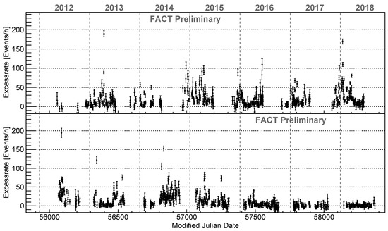
Figure 1.
Light curves of Mrk 421 (top) and Mrk 501 (bottom) measured by the first G-APD Cherenkov telescope (FACT). The vertical gray dashed lines indicate the start of a year.
In the context of AMON, FACT serves both as a triggering and follow-up instrument. In the past years, it already followed up five alerts delivered via AMON [10,11,12,13].
While those were alerts based on a stream by only one messenger (neutrinos measured by IceCube), future alerts will also include coincidences of two or more messengers, e.g., including alerts from FACT.
To allow for automatic alerts, FACT has an automatic quick-look analysis running onsite [14]. Thanks to a fast processing, alerts can be issued within 10–20 minutes after the data are stored to disk. For the alerts, two different streams have currently been set up, one based on 20-min binned light curves and one combining all data taken on one source in one night. For alerts to different telescopes, different algorithms and thresholds have been implemented to the automatic alert system. To determine the threshold for the alerts to AMON, one approach is to define the quiescent and active state of a source based on the flux distribution without applying an additional cut in significance of the data point.
2. Flux States
The probability density function (PDF) of the measured fluxes of a source, i.e., its flux distribution, is a powerful tool to characterize the emission of the source. In the following sections, an overview on existing studies based on the flux distribution of AGNs is given. Especially at VHE, only few results are available due to the relatively small number of sources and small data samples.
2.1. Shape of Flux Distribution
As described in [15], for additive processes, the fluxes are normally distributed, while multiplicative processes result in log-normal distributions. Like this, the shape of the flux distribution can give insights to the underlying processes. More details on this can be found in a separate article in this Special Issue [16], where previous studies are reviewed and a new study on the gamma-ray flux distributions of Mrk 501 is presented.
2.2. Steady State Emission
Many models assume that flares in AGN are individual events, e.g., caused by the injection of material which results in an enhanced flux. This implies also the existence of a steady state emission. For the flux distribution, this means that it consists of several components, one due to the steady-state emission and the rest due to activity of the source. Often, this steady-state emission is called the quiescent state of the source.
In [17], a normal distribution is assumed for the steady state emission and a log-normal distribution for the flares. Fitting the sum of these two functions to the data sample of a collection of public VHE data of Mrk 421, they calculate an upper limit for the quiescent state of 33% of the flux of the Crab Nebula at VHE.
Determining the steady state from the flux distribution, the sensitivity and systematics of the instrument also play a role and need to be considered.
2.3. Duty Cycle
Considering a steady state, the duty cycle of the source’s activity can be deduced. For this, the flux distribution is divided into a quiescent and active state, and the fraction of time a source spent in an active state is calculated.
In [18], the duty cycle for five blazars was calculated using RXTE/ASM data taken between 1996 and mid-2003. The highest duty cycle was found for Mrk 421 with about 22%. For 1ES 1959+650, a duty cycle of 17.5% was found, followed by H 1426+428 with about 16.5% and 1ES 2344+51.4 with about 16%. The lowest duty cycle was found for Mrk 501 with 14%. In [19], the duty cycle of 17 blazars was studied also in X-rays, finding duty cycles between 8% for 3C 279 and 27.3% for Mrk 421. This study also found that the blazars Mrk 501 and PKS 2155-304, which both have revealed very fast variability at VHE, have a relatively low duty cycle. This might, however, be biased by the data sample and the definition of the threshold (see below).
In [20], more than ten years of RXTE/ASM data were used to calculate the duty cycle of four blazars. They separated the flares from the characteristic flux level based on the distribution of flux states determined using maximum likelihood blocks. They did not use a specific shape to describe the flux distribution but used the peak of the distribution as a characteristic flux level. To determine the measurement uncertainty at low fluxes, flux distributions of faint sources were used. In this study, Mrk 421 was identified as the most active source with 40% of the time in an active state and 18% in a very high state, where they define the former as one sigma deviation from the characteristic flux and the latter three sigma. For Mrk 501, values of 26% and roughly 10% are found. 1ES 1959+650 flares less often, and 1ES 2155-304 is at the detection limit of RXTE/ASM, which makes conclusions difficult.
Based on a collection of existing VHE data of Mrk 421, the rate of high states was calculated depending on the flux level of the trigger threshold [21]. For a level of the flux of the Crab Nebula at TeV energies, a rate of flares of about 40% was obtained, decreasing to less than 10% for five times the flux of the Crab Nebula. However, this result is biased towards high fluxes due to the observing strategy (observations are typically triggered when the source is in a high state) and limited duty cycle of imaging air Cherenkov telescopes. Using water Cherenkov detectors, a more complete data sample can be collected. Based on Milagro data, the duty cycle was calculated depending on the baseline flux [22]. They found a result for Mrk 421 consistent with the X-ray result with a duty cycle of about 30% for a baseline flux of 33% of the flux of Crab Nebula. Comparing the results of the different studies, for the same source, different duty cycles are found. On the one hand, this can be due to different data samples; on the other hand, the result for the duty cycle depends on the definition of the threshold.
2.4. Definition of Threshold
To calculate the duty cycle, one needs to define a threshold for considering a state as active or high or to count a a flux state as a flare. For this, different approaches have been chosen in the various studies. In [18], the average flux has been used as a reference and everything that surpassed the average flux by 50% was considered as active. This description was also used in [19], requiring, in addition, a significance of at least three sigma for the deviation from the average flux. In [21], the high state rate, as they call it, was calculated in dependence of the threshold instead of choosing a specific threshold. The characteristic flux level from the distribution of flux states was determined in [20], and a spread of one sigma and three sigma was used as the threshold for the definition of the duty cycle. The same approach was used in [22], as it is independent of the average flux which might bias the result and makes it difficult to compare results from different sources and different energy bands.
2.5. Long-Term Monitoring
As the variability of AGN ranges from minutes to years, this also means that long-term observations are required to assess the steady state emission. For Mrk 421, a seasonal average flux ranging from 23% to 186% of the flux of the Crab Nebula at TeV energies was measured [23], illustrating nicely the long-term variations of the sources. Therefore, a long-term data sample is required to draw a complete picture.
Furthermore, it is crucial that the observations be unbiased with respect to the flux level.
At VHE, only a few instruments are available which have to deal with a variety of physics cases, limiting the time that can be spent on one source class and even more the time available for an individual object. To detect new sources, target-of-opportunity programs are used triggering VHE observations, e.g., from GeV or optical monitoring (e.g., [24,25]). While monitoring campaigns are carried out, for example, for the brightest blazars Mrk 421 and Mrk 501 with the large IACTs (see a detailed review in [26]), a lot of follow-up observations are still triggered in the case of flares. Due to this, the collected data samples are biased towards higher fluxes. In addition, monitoring of the large IACTs is limited to a short exposure, as discussed in [27]. To also characterize the low fluxes and steady state emission, unbiased long-term monitoring is needed.
The first monitoring at VHE was carried out by the Whipple 10-m telescope until 2009. From Mrk 421, 14 years of data were studied in [23].
Currently, there are two monitoring instruments at VHE. The first G-APD Cherenkov telescope (FACT) is using the imaging air Cherenkov technique to monitor a small sample of bright blazars. The high altitude water Cherenkov (HAWC) gamma-ray observatory observes 2/3 of the sky with the water Cherenkov technique. A detailed review of the monitoring at TeV energies is given in [9].
3. Data Sample from FACT Long-Term Monitoring
For the here presented study, data from the first G-APD Cherenkov telescope (FACT) were used considering the time range from October 2011 to September 2018. This makes a total of more than 11,700 h of physics data.
3.1. Sources
FACT is monitoring a small sample of blazars. In addition, the Crab Nebula is regularly observed for calibration purposes. The brightest blazars in the sample are Mrk 421, Mrk 501, 1ES 1959+650, and 1ES 2344+51.4. To study the flux uncertainties introduced by the measurement technique and the instrument, data of the Crab Nebula (steady source at TeV energies) and 1H 0323+342 (not detected at TeV energies) can be used.
The light curves of the brightest sources, Mrk 421 and Mrk 501, are shown in Figure 1 and the corresponding flux distributions in Figure 2.
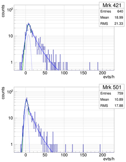
Figure 2.
Distributions of nightly fluxes of Mrk 421 (top) and Mrk 501 (bottom), as measured by FACT. In blue, the fit of the sum of a Gaussian and log-normal distribution is shown indicating in addition the two components as dashed blue lines. The fit of a Gaussian to the main part of the peak is shown in green. The crossing point of the two fits is marked with a circle.
3.2. Analysis and Data Selection
The data were analyzed as described in [28]. In addition, a data quality selection based on the cosmic-ray rate [29] was applied as described in [30]. This cut removed data suffering from bad weather or calima, resulting in data samples of 640 nights for Mrk 421 and 759 nights for Mrk 501 with more than 1700 h per source.
3.3. Determining the Steady State
Based on the flux distributions, the steady state of the sources is estimated. For this, the flux distributions are fitted with the sum of a Gaussian and a log-normal distribution (shown as blue solid line in Figure 2). To take into account the measurement uncertainty and the systematics of the instrument, the function is folded with a Gaussian distribution as the flux distributions of a steady source and a non-detected source follow a Gaussian distribution.
As the sources are not always detected within an individual night, the flux distributions extend to negative values (background fluctuations). Therefore, the value determined for steady state flux can be considered only as an upper limit.
3.4. Threshold for Flaring States
To determine the threshold which discriminates the steady state from active states, the fit of the sum of a Gaussian and log-normal distribution is compared to a fit of a Gaussian distribution to the main peak of the flux distribution (green solid line in Figure 2. The intersection of the two functions is defined as the trigger threshold (marked with a circle in Figure 2), as the function describing the full flux distributions starts at this point, deviating from the Gaussian describing the steady state.
4. Results
4.1. Mrk 421
Fitting the flux distribution of Mrk 421 from seven years of FACT monitoring, an upper limit for the steady state flux of 22% of the flux of the Crab Nebula at TeV energies was determined, which is lower than the upper limit from [17].
4.2. Mrk 501
Also for Mrk 501, an upper limit for the steady state flux was determined. Looking at the light curve in Figure 1, the flux shows the lowest level during the whole observation period in the years 2017 and 2018. Therefore, for the upper limit on the steady state flux, only the data of these two years are taken into account. Analyzing 538.7 h of data from 2017 and 2018 after data quality selection, a signal was only found with a significance of 4 sigma. Using the average flux of the two years, an upper limit on the steady state flux of 9% of the flux of the Crab Nebula at TeV energies was calculated. Calculating an upper limit on the average flux gives an upper limit of 15% of the Crab Nebula flux for the steady state. However, the flux distribution (see Figure 3) still shows some nights with a flux deviating from the main part of the flux distribution. Fitting the flux distribution with a Gaussian, an upper limit for the steady state flux of 2% of the flux of the Crab Nebula at TeV energies was determined.
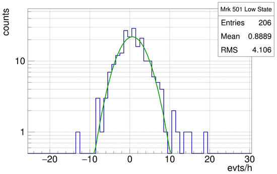
Figure 3.
Distribution of nightly fluxes of Mrk 501 in 2017 and 2018, as measured by FACT.
5. Multi-Messenger Context
For the correlation with other messengers, it is important to determine time ranges from the gamma-ray light curves during which neutrino emission might be expected.
5.1. Flux above Steady State
One approach is to determine the time ranges in which a source is in an active state, assuming that neutrinos are emitted whenever the source is active. As discussed earlier, there have been different approaches for the definition of an active state. Furthermore, the value of the threshold depends on a variety of influences as the sensitivity of the instrument and the completeness of the data sample. For example, a subset of a data sample measured during a longer-term high state would result in a too high threshold. The same happens if the data sample is biased towards higher fluxes due to target-of-opportunity observations of flares.
In the here presented study, the threshold to separate the active states from the steady state is determined by comparing a fit to the complete flux distribution (blue curve in Figure 2 with a fit to the steady state (green curve in Figure 2). The circle in the figure marks the point where the flux distribution starts deviating from a Gaussian distribution describing the steady state.
Using the flux distributions from seven years of monitoring, these points will be used as trigger thresholds for gamma-ray triggers to AMON. This type of triggers is being sent from FACT to AMON based on nightly and 20-min binning.
5.2. Trigger Threshold with Respect to Mean Flux
Assuming that not all activity in gamma rays causes neutrino emission, a different approach may be chosen. If only certain outbursts are associated to hadronic emission and therefore expect a correlation with neutrinos, gamma-ray triggers have to be defined differently.
Comparing the flux with mean flux of last x days (e.g., x = 30 or x = 365), short bright flares can be selected. This could be used as a separate trigger stream. Using the different streams for archival analysis and real-time triggers, the different physics cases can be tested.
6. Summary and Outlook
6.1. Steady State Flux
While for Mrk 421, a new upper limit for the steady state flux of 22% of the flux of the Crab Nebula at TeV energies has been determined, Mrk 501 was found in an extremely low state in 2017 and 2018. From this low state, an upper limit of 2% of the flux of the Crab Nebula at TeV energies was determined for the steady state flux.
Next, the study will be repeated using corrected excess rates in units of the Crab Nebula flux, improving the precision of the results. Further, for 1ES 1959+650 and 1ES 2344+51.4 flux, upper limits for the steady state emission will be determined.
6.2. Triggers to MWL and MM Instruments
To determine the threshold for a flaring state, the flux distributions are fitted with a sum of a Gaussian and a log-normal distribution. Comparing this to a Gaussian fit of the main part of the flux distribution, the point is determined from which the flux distribution starts deviating from a Gaussian distribution. This threshold will be used, for example, to send a gamma-ray trigger to the multi-messenger network AMON. Apart from this first alert stream which is currently being implemented, further alerts streams motivated by different physics cases are foreseen.
The study shows that unbiased long-term monitoring is crucial for the evaluation of flux distributions to determine characteristics as the source’s duty cycle.
Author Contributions
D.D. carried out the presented study and wrote the paper. All members of the FACT Collaboration contributed to building and/or maintaining the instrument and/or taking the data.
Funding
The important contributions from ETH Zurich grants ETH-10.08-2 and ETH-27.12-1 as well as the funding by the Swiss SNF and the German BMBF (Verbundforschung Astro- und Astroteilchenphysik) and HAP (Helmoltz Alliance for Astroparticle Physics) are gratefully acknowledged. Part of this work is supported by Deutsche Forschungsgemeinschaft (DFG) within the Collaborative Research Center SFB 876 “Providing Information by Resource-Constrained Analysis”, project C3.
Acknowledgments
We are thankful for the very valuable contributions from E. Lorenz, D. Renker and G. Viertel during the early phase of the project. We thank the Instituto de Astrofísica de Canarias for allowing us to operate the telescope at the Observatorio del Roque de los Muchachos in La Palma, the Max-Planck-Institut für Physik for providing us with the mount of the former HEGRA CT3 telescope, and the MAGIC collaboration for their support.
Conflicts of Interest
The authors declare no conflict of interest.
References
- Böttcher, M. Progress in Multi-wavelength and Multi-Messenger Observations of Blazars and Theoretical Challenges. Galaxies 2019, 7, 20. [Google Scholar] [CrossRef]
- Garcia-Gonzalez, J. X-ray/gamma-ray Correlation in Blazars. Galaxies 2019. submitted. [Google Scholar]
- IceCube Collaboration. Evidence for High-Energy Extraterrestrial Neutrinos at the IceCube Detector. Science 2013, 342, 1242856. [Google Scholar] [CrossRef] [PubMed]
- IceCube Collaboration; Aartsen, M.G.; Ackermann, M.; Adams, J.; Aguilar, J.A.; Ahlers, M.; Ahrens, M.; Al Samarai, I.; Altmann, D.; Andeen, K.; et al. Multimessenger observations of a flaring blazar coincident with high-energy neutrino IceCube-170922A. Science 2018, 361, eaat1378. [Google Scholar] [CrossRef]
- Kintscher, T.; Icecube Collaboration; Fact Collaboration; MAGIC Collaboration; Krings, K.; Dorner, D.; Bhattacharyya, W.; Takahashi, M. IceCube Search for Neutrinos from 1ES 1959+650: Completing the Picture. In Proceedings of the International Cosmic Ray Conference, Bexco, Busan, Korea, 10–20 July 2017; Volume 35, p. 969. [Google Scholar]
- Ayala Solares, H. AMON Multimessenger Alerts: Past and Future. Galaxies 2019, 7, 19. [Google Scholar] [CrossRef]
- Anderhub, H.; Backes, M.; Biland, A.; Boccone, V.; Braun, I.; Bretz, T.; Buß, J.; Cadoux, F.; Commichau, V.; Djambazov, L.; et al. Design and operation of FACT—The first G-APD Cherenkov telescope. J. Instrum. 2013, 8, P06008. [Google Scholar] [CrossRef]
- Biland, A.; Bretz, T.; Buß, J.; Commichau, V.; Djambazov, L.; Dorner, D.; Einecke, S.; Eisenacher, D.; Freiwald, J.; Grimm, O.; et al. Calibration and performance of the photon sensor response of FACT—The first G-APD Cherenkov telescope. J. Instrum. 2014, 9, P10012. [Google Scholar] [CrossRef]
- Dorner, D.; Gonzalez, M.; Bretz, T. Unbiased Long-Term Monitoring at TeV Energies. Galaxies 2019, 7, 51. [Google Scholar]
- Biland, A. FACT Follow-Up of IceCube20181023A. Available online: https://gcn.gsfc.nasa.gov/gcn3/23401.gcn3 (accessed on 9 May 2019).
- Biland, A. FACT Follow-Up of IceCube20171106; GRB Coordinates Network, Circular Service, No. 22120, #1 (2017). 2017; p. 22120. Available online: https://gcn.gsfc.nasa.gov/gcn3_archive.html (accessed on 9 May 2019).
- Biland, A. FACT Follow-Up of IceCube20160731; GRB Coordinates Network, Circular Service, No. 19752, #1 (2016). 2016; p. 19752. Available online: https://gcn.gsfc.nasa.gov/gcn3_archive.html (accessed on 9 May 2019).
- Biland, A.; Dorner, D. FACT Follow-Up of the IceCube Event 160427A; GRB Coordinates Network, Circular Service, No. 19427, #1 (2016). 2016; p. 19427. Available online: https://gcn.gsfc.nasa.gov/gcn3_archive.html (accessed on 9 May 2019).
- Dorner, D.; Biland, A.; Bretz, T.; Buss, J.; Einecke, S.; Eisenacher, D.; Hildebrand, D.; Knötig, M.L.; Krähenbühl, T.; Lustermann, W.; et al. FACT—Long-term Monitoring of Bright TeV-Blazars. arXiv 2013, arXiv:astro-ph.HE/1311.0478. [Google Scholar]
- Uttley, P.; McHardy, I.M.; Vaughan, S. Non-linear X-ray variability in X-ray binaries and active galaxies. Mon. Not. R. Astron. Soc. 2005, 359, 345–362. [Google Scholar] [CrossRef]
- Romoli, C.; Chakraborty, N.; Dorner, D.; Taylor, A.M.; Blank, M. Flux Distribution of Gamma-Ray Emission in Blazars: The Example of Mrk 501. Galaxies 2018, 6, 135. [Google Scholar] [CrossRef]
- Tluczykont, M.; Bernardini, E.; Satalecka, K.; Clavero, R.; Shayduk, M.; Kalekin, O. Long-term lightcurves from combined unified very high energy γ-ray data. Astron. Astrophys. 2010, 524, A48. [Google Scholar] [CrossRef]
- Krawczynski, H.; Hughes, S.B.; Horan, D.; Aharonian, F.; Aller, M.F.; Aller, H.; Boltwood, P.; Buckley, J.; Coppi, P.; Fossati, G.; et al. Multiwavelength Observations of Strong Flares from the TeV Blazar 1ES 1959+650. Astrophys. J. 2004, 601, 151–164. [Google Scholar] [CrossRef]
- Wagner, R.M. Synoptic studies of 17 blazars detected in very high-energy γ-rays. Mon. Not. R. Astron. Soc. 2008, 385, 119–135. [Google Scholar] [CrossRef]
- Resconi, E.; Franco, D.; Gross, A.; Costamante, L.; Flaccomio, E. The classification of flaring states of blazars. Astron. Astrophys. 2009, 502, 499–504. [Google Scholar] [CrossRef]
- Tluczykont, M.; Shayduk, M.; Kalekin, O.; Bernardini, E. Long-term gamma-ray lightcurves and high state probabilities of Active Galactic Nuclei. J. Phys. Conf. Ser. 2007, 60, 318–320. [Google Scholar] [CrossRef]
- Abdo, A.A.; Abeysekara, A.U.; Allen, B.T.; Aune, T.; Barber, A.S.; Berley, D.; Braun, J.; Chen, C.; Christopher, G.E.; Delay, R.S.; et al. The Study of TeV Variability and the Duty Cycle of Mrk 421 from 3 yr of Observations with the Milagro Observatory. Astrophys. J. 2014, 782, 110. [Google Scholar] [CrossRef]
- Acciari, V.A.; Arlen, T.; Aune, T.; Benbow, W.; Bird, R.; Bouvier, A.; Bradbury, S.M.; Buckley, J.H.; Bugaev, V.; de la Calle Perez, I.; et al. Observation of Markarian 421 in TeV gamma rays over a 14-year time span. Astropart. Phys. 2014, 54, 1–10. [Google Scholar] [CrossRef]
- Albert, J.; Aliu, E.; Anderhub, H.; Antoranz, P.; Armada, A.; Asensio, M.; Baixeras, C.; Barrio, J.A.; Bartko, H.; Bastieri, D.; et al. Discovery of Very High Energy γ-Rays from Markarian 180 Triggered by an Optical Outburst. Astrophys. J. Lett. 2006, 648, L105–L108. [Google Scholar] [CrossRef]
- Cerruti, M.; Lenain, J.P.; Prokoph, H.; H.E.S.S. Collaboration. H.E.S.S. discovery of very-high-energy emission from the blazar PKS 0736+017: On the location of the γ-ray emitting region in FSRQs. In Proceedings of the International Cosmic Ray Conference, Bexco, Busan, Korea, 10–20 July 2017; Volume 35, p. 627. [Google Scholar]
- Paneque, D. Unravelling the complex behaviour of our closest very-high-energy gamma-ray blazars, Mrk421 and Mrk501. Galaxies. 2019. Available online: https://indico.scc.kit.edu/event/390/contributions/4474/attachments/2282/3170/Paneque_MWMrks_Cochem_v2.pdf (accessed on 9 May 2019).
- Dorner, D.; Ahnen, M.L.; Balbo, M.; Bergmann, M.; Biland, A.; Bretz, T.; Brügge, K.A.; Buss, J.; Einecke, S.; Freiwald, J.; et al. FACT—TeV Flare Alerts Triggering Multi-Wavelength Observations. In Proceedings of the 34th International Cosmic Ray Conference (ICRC2015), The Hague, The Netherlands, 30 July–6 August 2015; Volume 34, p. 704. [Google Scholar]
- Dorner, D.; Ahnen, M.L.; Bergmann, M.; Biland, A.; Balbo, M.; Bretz, T.; Buss, J.; Einecke, S.; Freiwald, J.; Hempfling, C.; et al. FACT—Monitoring Blazars at Very High Energies. arXiv 2015, arXiv:astro-ph.IM/1502.02582. [Google Scholar]
- Hildebrand, D.; Ahnen, M.L.; Balbo, M.; Biland, A.; Bretz, T.; Buss, J.; Dorner, D.; Einecke, S.; Elsaesser, D.; Herbst, T.; et al. Using Charged Cosmic Ray Particles to Monitor the Data Quality of FACT. In Proceedings of the International Cosmic Ray Conference, Busan, Korea, 10–20 July 2017; Volume 35, p. 779. [Google Scholar]
- Mahlke, M.; Bretz, T.; Adam, J.; Ahnen, L.M.; Baack, D.; Balbo, M.; Biland, A.; Blank, M.; Bruegge, K.; Buss, J.; et al. FACT—Searching for periodicity in five-year light-curves of Active Galactic Nuclei. In Proceedings of the International Cosmic Ray Conference, Busan, Korea, 10–20 July 2017; Volume 35, p. 612. [Google Scholar]
| 1. | Status in September 2018, as presented at the conference. |


© 2019 by the authors. Licensee MDPI, Basel, Switzerland. This article is an open access article distributed under the terms and conditions of the Creative Commons Attribution (CC BY) license (http://creativecommons.org/licenses/by/4.0/).