Faraday Depolarization Effects in Spiral Galaxies

Abstract

Magnetic fields in the universe play an essential role in observations of the radio synchrotron continuum; however, we do not know enough about them, either observationally or theoretically. We are interested in galactic magnetic fields because they affect the structural formation of galaxies in terms of star-forming regions, spiral arms, and threads at the galactic center. To clarify the importance of magnetic fields, we carried out numerical simulations of the galactic gaseous disk with magnetic fields. We also calculated observables, such as the rotation measure and Stokes parameters, from the results of numerical simulation. FD maps and intensity maps have been reported, and the relation between azimuthal angle and FD has been shown to depend on the inclination of the observer. Furthermore, it has been shown that a polarized intensity below 800 MHz reflects field structure in the halo region, although the intensity is weak. The present paper summarizes the effects of Faraday depolarization and the relation between magnetic-field structure and Stokes parameters.

1. Introduction

Spiral galaxies have spiral arms in which the strength of magnetic fields is on the order of a microgauss $\mathsf{\mu }$G. The origin of such global magnetic fields in spiral galaxies is under discussion, but the most likely models are based on dynamo theories [1,2]. Several numerical simulations have been performed to reveal the maintenance mechanism of the magnetic fields [3]. These simulations produced a quasisteady state with a field strength of a few microgauss, similar to the observational results, though the mechanisms of amplification differed among the simulations.

The topology of the magnetic field of a galaxy is classified by the relation between azimuthal angle and Faraday rotation measure (RM) (e.g., as an axisymmetric spiral (ASS) as seen in M31, or bisymmetric spiral (BSS) as possibly seen in M81). Because the observed intensity is integrated along the line of sight (LOS), the components along the LOS cannot be directly separated. Faraday tomography recently revealed that the magnetic-field topology of M51 has the characteristics of both an ASS and BSS [4]. The magnetic-field strength of the global feature becomes higher than a few microgauss and turbulent components coexist in the grand design spiral [5]. The effect of superposition along the LOS is diminishing with the development of new techniques. However, a mapping between the Faraday depth (FD) and spatial length is still needed to know the real distribution.

Observational visualization is a powerful way of presenting information of the relation between the FD and the distribution of the physical gas and magnetic-field distributions. Machida et al. (2018a) (Reference [6], hearafter Paper I) and Machida et al. (2018b) (Reference [7], hearafter Paper II) reported a synthetic observational analysis of spiral galaxies using the spatial distribution of physical values used in numerical simulation. They assumed that the radio signal is a synchrotron emission from background radio sources. They showed that the classification of the dependence of the RM on the azimuthal angle depends on the inclination of the LOSI, i.e., a spiral is classified as an ASS with higher modes when observed at a viewing angle of <70${}^{\circ }$, while an edge-on view presents a ringlike structure. In addition, they calculated the effect of Faraday depolarization and showed a polarized intensity ranging from 100 MHz to 10 GHz.

The present paper summarizes the results of the magnetic-field structure and polarized intensity. Calculation methods are presented in Section 2, while numerical results are presented in Section 3. Section 4 and Section 5 are a discussion and summary.

2. Numerical Methods

The numerical results that we adopted are the results of a global magnetohydrodynamic simulation of a galactic gaseous disk [8]. The simulation units of density, velocity, and length are, respectively, ${\rho }_0=1.6\times {10}^{-24}\mathrm{g}{\mathrm{cm}}^{-3}$, $v_0=207\mathrm{km}/\mathrm{s}$, and $r_0=1\mathrm{kpc}$. Because magnetic-field strength is defined by the plasma $\beta$, which is the ratio of gas pressure to magnetic pressure, the unit strength of the magnetic field is proportional to the density $B_0=\sqrt{{\rho }_0{v}_0^2}=26\mathsf{\mu }\mathrm{G}$. The gas is assumed to be adiabatic, and we ignore cooling and heating effects. This assumption is unrealistic for the temperature distribution of the gas. In this paper, we assume that the turbulent motion of warm neutral gas is approximated by the motion of warm ionized gas, because the velocity dispersion of the turbulent motion is comparable to the speed of sound in warm ionized gas. After magnetic turbulence develops in the disk and the disk becomes quasisteady, plasma $\beta$ becomes $\beta$∼10–20, and the averaged density in the disk is about $0.01{\mathrm{cm}}^{-3}$. Details of the numerical simulations have been published in Reference [8] and Appendix A of Paper I.

We obtained the Stokes parameters and FD from physical values of the numerical model. The galactic center is set on the center of the co-ordinates, and inclination angle $\theta$ is the angle from the rotational axis. The inclined axis is chosen to be the z-axis in the calculation box. The face-on view is chosen as $\theta =5^{\circ }$ and the edge-on view as $\theta ={85}^{\circ }$. The computational domain comprises 20 kpc cubes $(i,j,k)$ in Cartesian co-ordinates that are interpolated from cylindrical coordinates. The spatial resolution is 100 pc. The FD and Stokes parameters are integrated from the upper boundary $k=200$ and projected on the bottom plain (k = 0).

The procedure of observational visualization is as follows:

• The FD along the LOS is integrated from the local FD within a computational cell. To include Faraday depolarization, we calculated two types of FD. The mean FD corresponds to the global component of magnetic field $\overline{B}$, and the turbulent FD is calculated as the turbulent component of the magnetic field $b=B-\overline{B}$:

  $$F{D}_{\mathrm{ave},i,j,k}=\sum _{l=1}^{k}0.81n_{\mathrm{e}}{\overline{B}}_{\parallel }\Delta l,$$

  (1)

  and

  $$F{D}_{\mathrm{turb},i,j,k}=\sum _{l=1}^{k}0.81n_{\mathrm{e}}{b}_{\parallel }\Delta l.$$

  (2)

  Here, $n_{\mathrm{e}}$, $B_{\left|\right|}$, and $\Delta l$ are, respectively, the number density of free electrons, LOS component of the magnetic field, and line elements $\Delta l=100$ pc. To calculate the mean field, the magnetic field is averaged over an area of $\pm 5$ cells from the central cell. We discuss the dependence of the mean components of magnetic fields on the averaging region in Section 4.1 of Paper II.
• We calculate the internal and external Faraday depolarization [9],

  $$D_{\mathrm{i}}=\left(\frac{1-exp(-2{\sigma }_{F{D}_{i,j,k}}^2{\lambda }^4)}{2{\sigma }_{F{D}_{i,j,k}}^2{\lambda }^4}\right)$$

  (3)

  and

  $$D_{\mathrm{e}}=exp(-2{\sigma }_{\mathrm{FD},\mathrm{i},\mathrm{j},\delta \mathrm{l}}^2{\lambda }^4)$$

  (4)

  respectively, where $\lambda$ is the wavelength and ${\sigma }_{F{D}_{i,j,\delta l}}$ is the dispersion of the local $F{D}_{i,j,\delta l}$. ${\sigma }_{{\mathrm{FD}}_{\mathrm{i},\mathrm{j},\mathrm{k}}}$ is the dispersion at grid point $(i,j,k)$.
• We obtain the frequency-independent Faraday depolarization [10], which is determined by the degree of intrinsic polarization:

  $$W=\frac{1+3.5q^2}{1+4.5q^2+2.5q^4},$$

  (5)

  where $q=\overline{b_{\perp }}/\overline{B_{\perp }}$ is the ratio of the turbulent component to the mean field perpendicular to the LOS.
• We calculate the polarization position angles.
• We calculate the Stokes parameters of synchrotron radiation emitted at the k-th cell. These parameters are included in the internal Faraday depolarization, external Faraday depolarization, frequency-independent depolarization, and free–free absorption of synchrotron emission.

Detailed treatments are presented in Papers I and II.

The present paper assumes that the energy density of cosmic rays is equal to the energy density of the magnetic field [11] and assumes the energy spectral index of the cosmic rays is $p=3$ [12].

3. Results

3.1. Relation between the FD and the LOS Components of the Magnetic Field

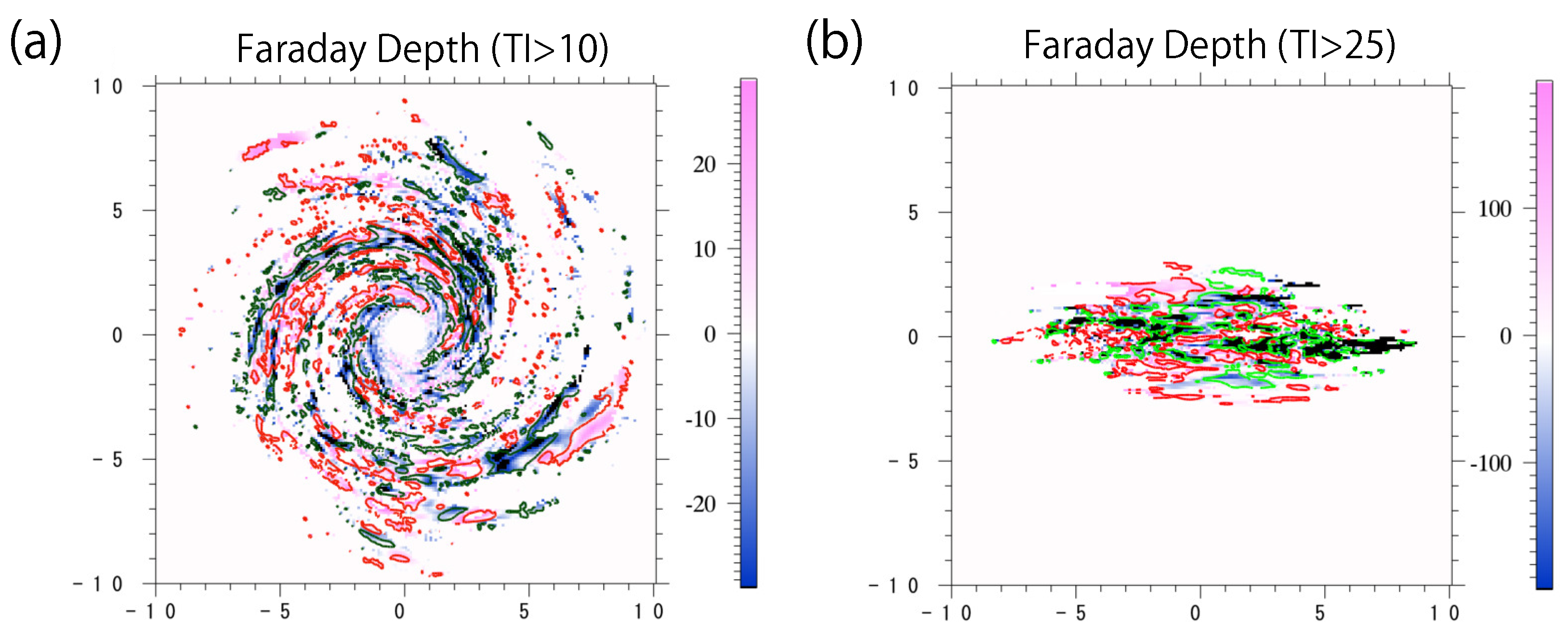
Figure 1 shows the distribution of the FD where the total intensity at a frequency of 1.58 GHz is greater than the average intensity. The contours plotted in the panels denote the magnetic field-component parallel to the LOS, averaged along the LOS. Red and green contours, respectively, show components in positive and negative directions with respect to the LOS. Figure 1a,b respectively shows the face-on case and edge-on case. Detailed distributions of FD maps are presented in Figures 2 and 3 of paper I. In the face-on case, the direction of the FD is almost consistent with the direction of the magnetic field; however, some regions have a complicated structure. For example, the LOS field direction is negative in the region around $(5,-5)$, and yet part of the FD becomes positive. Additionally, the FD around $(0,-2)$ has a complicated structure. The LOS components have negative structure around that region, although it are not shown by the contour lines. A similar tendency is seen around the y-axis in the case of the edge-on spiral galaxy.

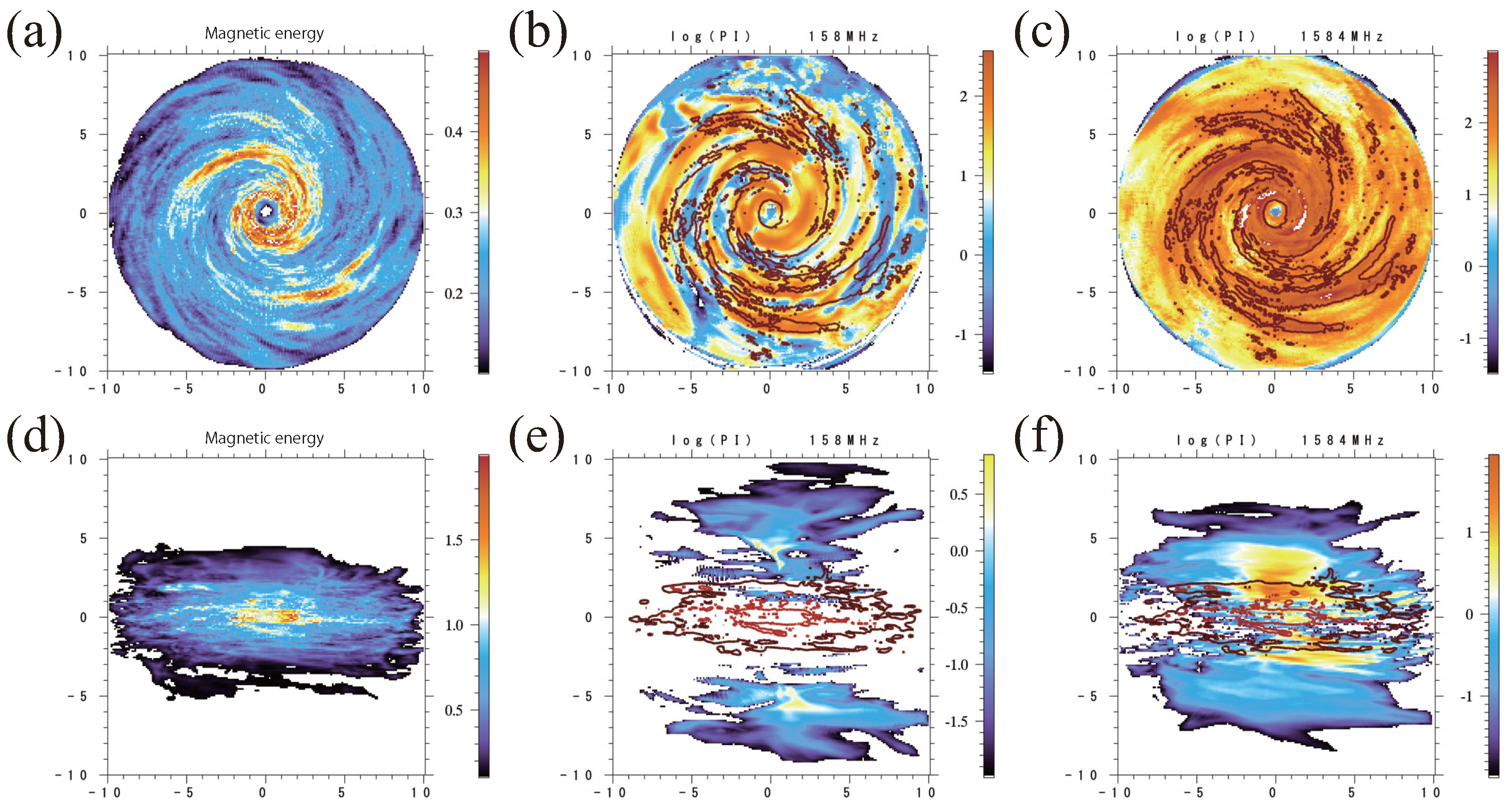
3.2. Relation between Polarized Intensity and Magnetic Energy

Figure 2a,d shows the magnetic energy integrated along the LOS. The top and bottom rows, respectively, show the face-on view and edge-on view. In the face-on case, the magnetic energy has spiral arms. The dominant components of the magnetic field are the azimuthal components. The turbulent components are overlaid on the mean fields. The magnetic fields are strongest around the equatorial plane; however, the strength of the halo fields are a few 10% of the strength of the equatorial fields (see Figure 5 in Paper I). This is because the magnetic fields amplified by the magnetorotational instability float to the halo through the Parker instability when the magnetic pressure becomes comparable to the gas pressure. The buoyantly rising magnetic flux expands in the halo, and the field becomes weaker than that in the disk.

The middle and right panels of Figure 2 show contours of magnetic energy plotted over maps of polarized intensity for frequencies of 158 MHz and 1.58 GHz, respectively. The unit of polarized intensity is $\mathsf{\mu }$Jy/beam, where we assume a beam having a diameter of 10 arcsec. In the case of the face-on view, polarized intensity is proportional to the magnetic energy because the main part of the magnetic energy corresponds to the components of the field perpendicular to the LOS. Depolarization does not have an effect at higher frequency, although the polarization angle is rotated from the original direction (see Figure 3 in Paper II). Meanwhile, because depolarization has an effect at low frequency, the polarized intensity becomes weak around the region with strong magnetic energy (e.g., see around (−5, −1–4)). Meanwhile, polarized intensity in the edge-on spiral does not only scale with the distribution of the magnetic energy. The main effect of depolarization is weighted by that of the gas density. The gas density in the central region is underestimated because we adopted absorbing boundary conditions at the center, although the central region may also depolarize at 1.58 GHz when we include the effect of molecular cooling.

4. Discussion

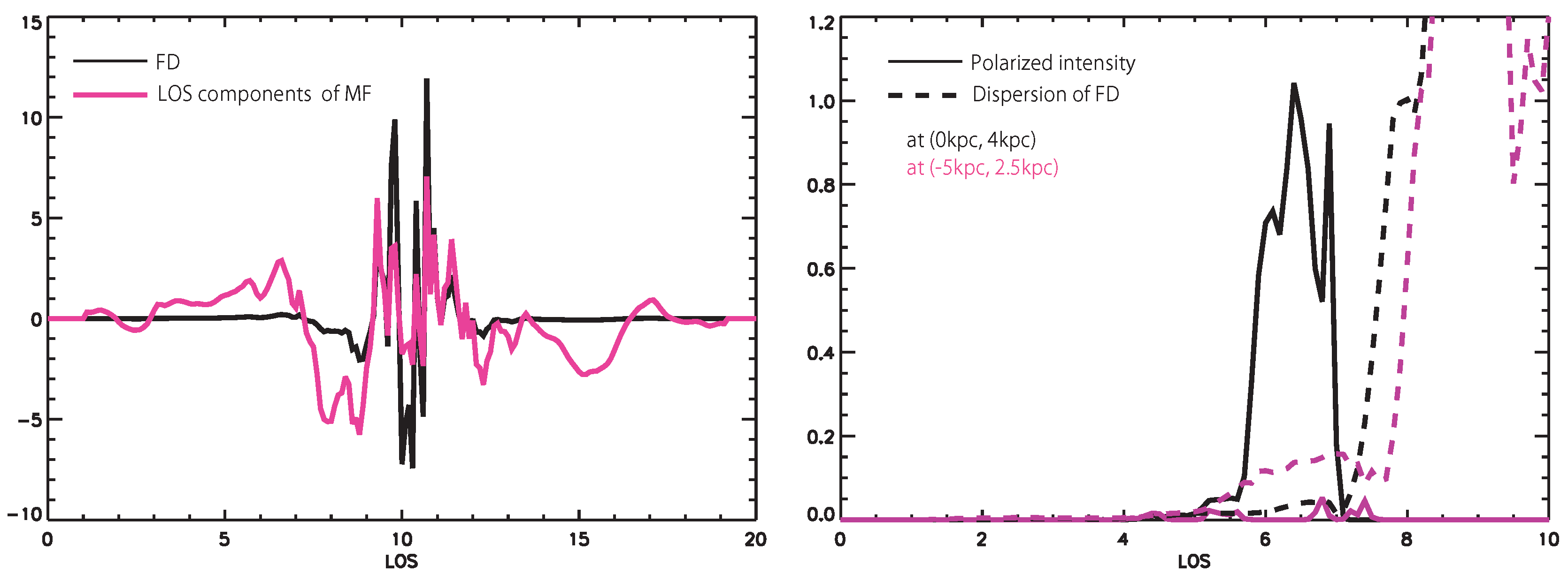
We consider why the FD has complex features within a contour of the same direction for the LOS magnetic field. The left panel in Figure 3 shows the LOS distribution of the FD (black) and the magnetic field parallel to the LOS (magenta) at $(0\mathrm{kpc},1\mathrm{kpc})$. This region has a positive value of the FD but a negative value of the LOS component of the magnetic field. This is because the FD is defined by the product of the density and the LOS component of the magnetic field. The FD has peaks around the equatorial plane (LOS∼10), and strength decreases approaching LOS∼8, which is 3 kpc from the equatorial plane. Meanwhile, the magnetic field has comparable strength in the disk and halo. Although the integrated field shows one direction, the magnetic field changes direction along the LOS. Maximum strength becomes 7 $\mathsf{\mu }$G, while the integrated value at $(0\mathrm{kpc},1\mathrm{kpc})$ is about 0.2 $\mathsf{\mu }$G. This means that the magnetic-field strength is underestimated from the synthetic observation.

The discrepancy between the FD and the parallel component of the magnetic field is not remarkable in the edge-on case. Because of the effect of inclination, the LOS component is parallel to the azimuthal component, which is dominant in the galactic disk. The direction of the azimuthal field reverses with increasing radius. There are reversals of the LOS component; however, the LOS component becomes largest along the LOS parallel to the tangential direction at that radius, and the density at the tangential point becomes largest along the LOS. The signs of the FD and LOS components, therefore, indicate a similar direction.

We next consider depolarization at low frequency. The right panel of Figure 3 shows the LOS distribution of the polarized intensity at 158 MHz (solid curves) and the dispersion of the FD (dashed curves). Black curves denote the position where the polarized intensity at 158 MHz is strong and magenta curves show that where the polarized intensity becomes weak, although both regions have a strong polarized intensity at 1.58 GHz. We find the origin of the polarized intensity is located 3 kpc from the equatorial plane. When the dispersion of the FD increases gradually, the polarized intensity suddenly decreases owing to depolarization at $(0\mathrm{kpc},4\mathrm{kpc})$. Polarized intensity at 1.58 GHz originates from the equatorial plane. Meanwhile, the dispersion of the FD increases rapidly in the region of low polarized intensity. These two regions have similar values of the LOS field and RM, although they have different strengths for the turbulent components. There is, thus, depolarization, and the polarized intensity decreases. This indicates that the polarized intensity relates to the halo region, such that we can obtain information about the halo magnetic field. The estimated intensity is about a few 10 $\mathsf{\mu }$Jy/beam, which is difficult to detect with current observatories. In the era of the Square Kilometre Array, however, halo magnetic fields are observable at low frequency.

5. Conclusions

We summarized our synthetic observational analysis of numerical simulations.

• The FD has a complicated structure for both face-on and edge-on spiral galaxies. There is FD reversal along the magnetic spiral arms. FD direction often follows the direction of the LOS component of the magnetic field; however, the FD does not always correlate with the magnetic field. This is because the magnetic field has inversions along the LOS and a similar strength from 5 km across the equatorial plane. Meanwhile, density has peaks around the equatorial plane.
• Polarized intensity correlates with the structure of the magnetic energy when the observed frequency is sufficiently high. At low frequency, the polarized intensity partially disappears owing to Faraday depolarization.

References

- Parker, E.N. The Generation of Magnetic Fields in Astrophysical Bodies. I. The Dynamo Equations. Astrophys. J. 1970, 162, 665. [Google Scholar] [CrossRef]
- Parker, E.N. The Generation of Magnetic Fields in Astrophysical Bodies. II. The Galactic Field. Astrophys. J. 1971, 163, 255. [Google Scholar] [CrossRef]
- Hanasz, M.; Wóltański, D.; Kowalik, K. Global Galactic Dynamo Driven by Cosmic Rays and Exploding Magnetized Stars. Astrophys. J. Lett. 2009, 706, L155–L159. [Google Scholar] [CrossRef]
- Fletcher, A.; Beck, R.; Shukurov, A.; Berkhuijsen, E.M.; Horellou, C. Magnetic fields and spiral arms in the galaxy M51. Mon. Not. R. Astron. Soc. 2011, 412, 2396–2416. [Google Scholar] [CrossRef]
- Beck, R. Magnetism in the spiral galaxy NGC 6946: Magnetic arms, depolarization rings, dynamo modes, and helical fields. Astron. Astrophys. 2007, 470, 539–556. [Google Scholar] [CrossRef]
- Machida, M.; Akahori, T.; Nakamura, K.E.; Nakanishi, H.; Haverkorn, M. Radio broadband visualization of global three-dimensional magnetohydrodynamical simulations of spiral galaxies-I. Faraday rotation at 8 GHz. Mon. Not. R. Astron. Soc. 2018, 480, 17–25. [Google Scholar] [CrossRef]
- Machida, M.; Akahori, T.; Nakamura, K.E.; Nakanishi, H.; Haverkorn, M. Radio broad-band visualization of global three-dimensional magnetohydrodynamical simulations of spiral galaxies–II. Faraday depolarization from 100 MHz to 10 GHz. Mon. Not. R. Astron. Soc. 2019, 482, 3394–3402. [Google Scholar] [CrossRef]
- Machida, M.; Nakamura, K.E.; Kudoh, T.; Akahori, T.; Sofue, Y.; Matsumoto, R. Dynamo Activities Driven by Magnetorotational Instability and the Parker Instability in Galactic Gaseous Disks. Astrophys. J. 2013, 764, 81. [Google Scholar] [CrossRef]
- Arshakian, T.G.; Beck, R. Optimum frequency band for radio polarization observations. Mon. Not. R. Astron. Soc. 2011, 418, 2336–2342. [Google Scholar] [CrossRef]
- Sokoloff, D.D.; Bykov, A.A.; Shukurov, A.; Berkhuijsen, E.M.; Beck, R.; Poezd, A.D. Depolarization and Faraday effects in galaxies. Mon. Not. R. Astron. Soc. 1998, 299, 189–206. [Google Scholar] [CrossRef]
- Akahori, T.; Kato, Y.; Nakazawa, K.; Ozawa, T.; Gu, L.; Takizawa, M.; Fujita, Y.; Nakanishi, H.; Okabe, N.; Makishima, K. ATCA 16 cm observation of CIZA J1358.9-4750: Implication of merger stage and constraint on non-thermal properties. Publ. Astron. Soc. Jpn. 2018, 70, 53. [Google Scholar] [CrossRef]
- Sun, X.H.; Reich, W.; Waelkens, A.; Enßlin, T.A. Radio observational constraints on Galactic 3D-emission models. Astron. Astrophys. 2008, 477, 573–592. [Google Scholar] [CrossRef]
© 2019 by the authors. Licensee MDPI, Basel, Switzerland. This article is an open access article distributed under the terms and conditions of the Creative Commons Attribution (CC BY) license (http://creativecommons.org/licenses/by/4.0/).