Faraday Tomography of the SS433 Jet Termination Region

 , ,
, , 
Abstract
1. Introduction
2. Observation and Model
2.1. Observation
2.2. Model
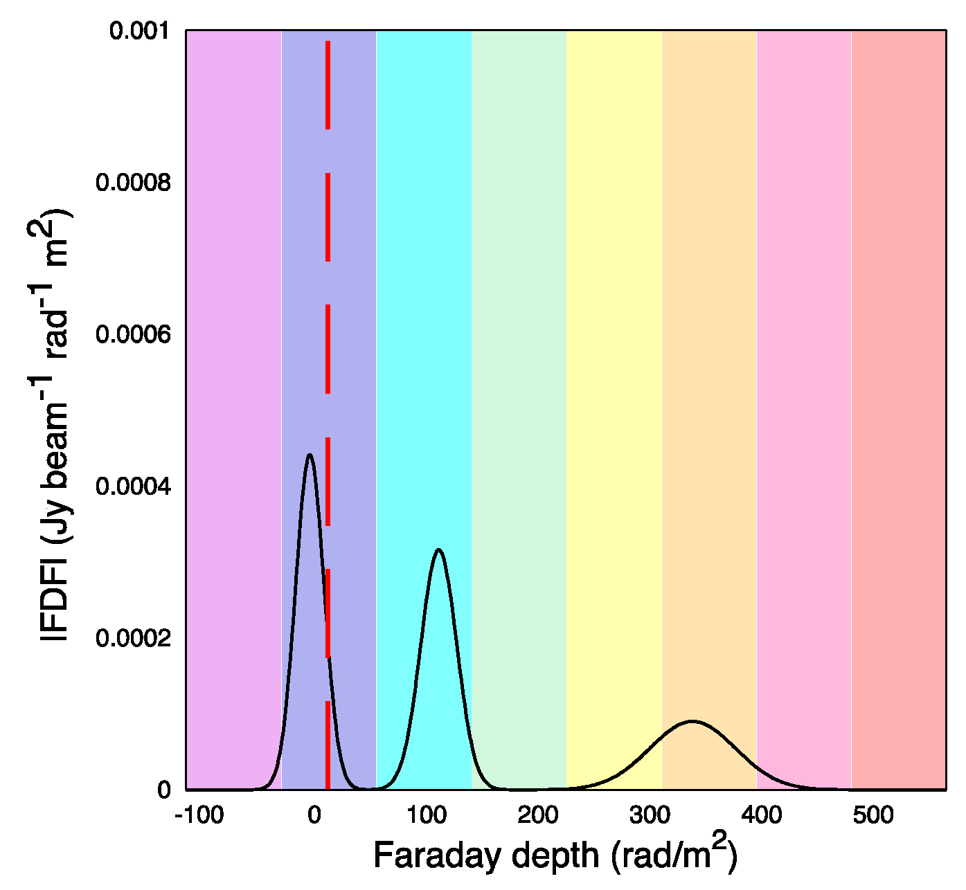
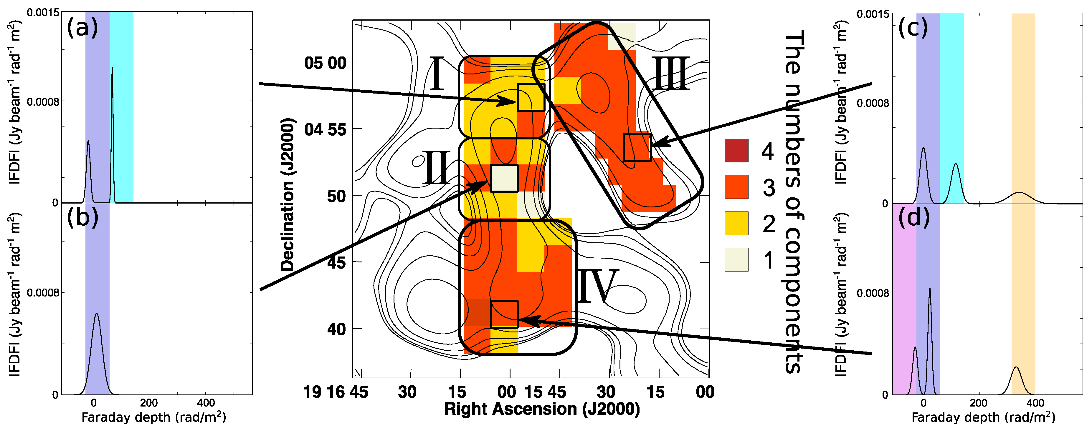
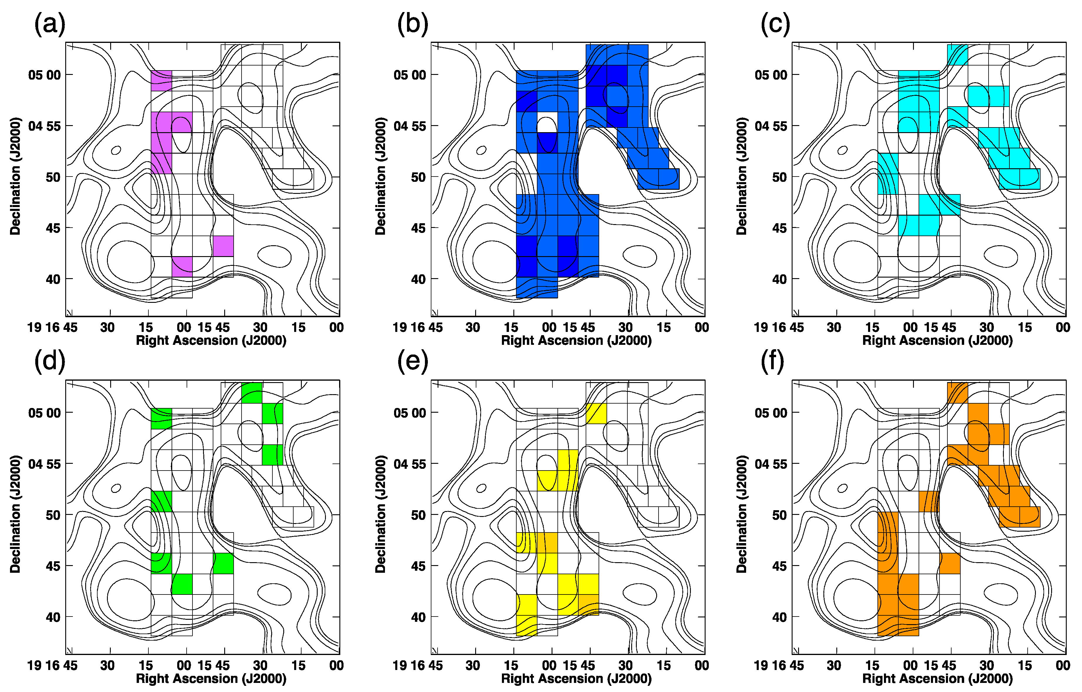
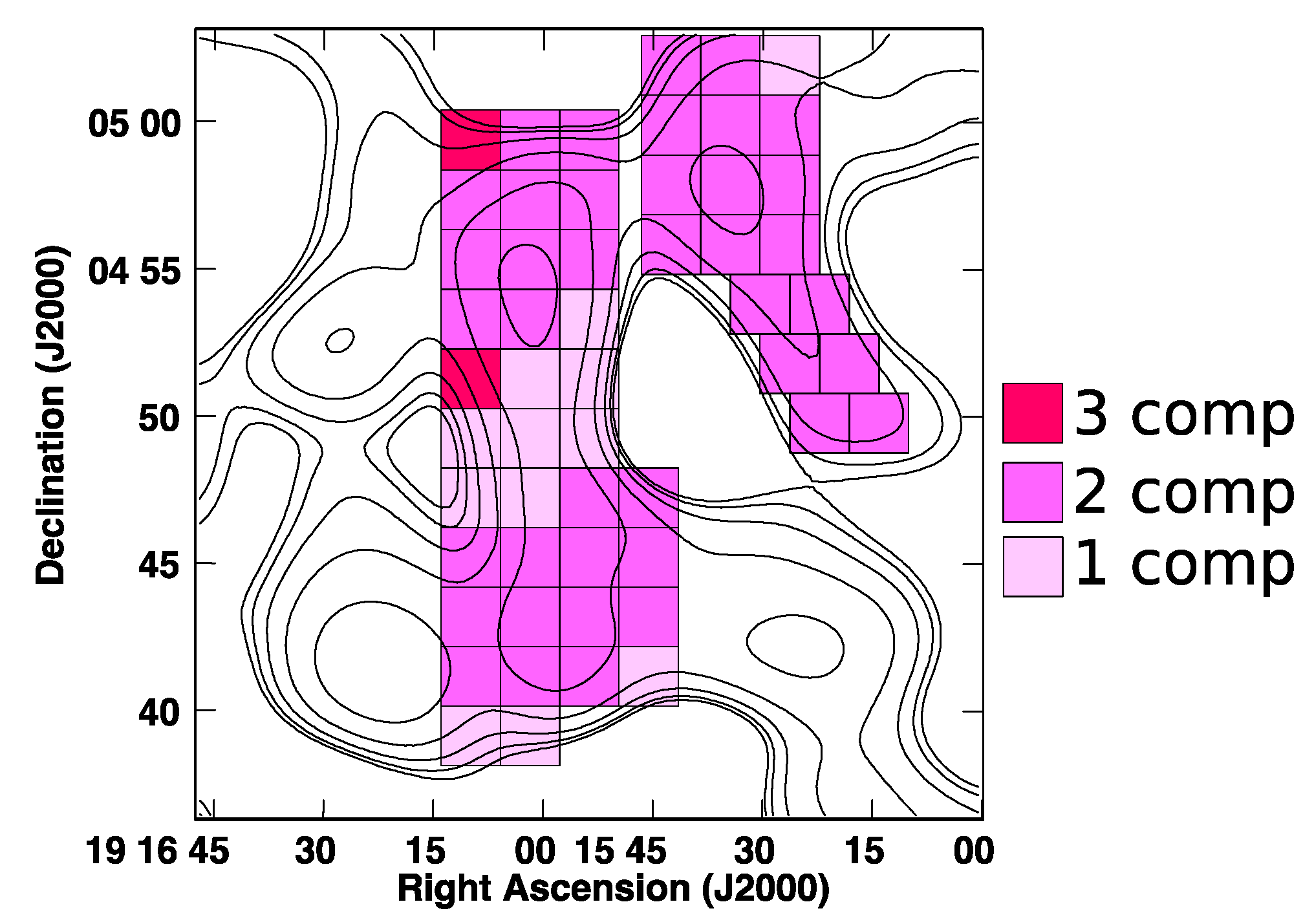
3. Results
4. Discussion
5. Conclusions
Author Contributions
Funding
Acknowledgments
Conflicts of Interest
References
- Araudo, A.T.; Bell, A.R.; Blundell, K.M. Particle Acceleration and Magnetic Field Amplification in the Jets of 4C74.26. Astrophys. J. 2015, 806, 243. [Google Scholar] [CrossRef]
- Abeysekara, A.U.; Albert, A.; Alfo, R.; HAWC Collaboration. Very high energy particle acceleration powered by the jets of the microquasar SS 433. Nature 2018, 562, 82–85. [Google Scholar] [CrossRef] [PubMed]
- Abell, G.O.; Margon, B. A kinematic model for SS433. Nature 1979, 279, 701–703. [Google Scholar] [CrossRef]
- Geldzahler, B.J.; Pauls, T.; Salter, C.J. Continuum observations of the supernova remnants W 50 and G 74.9+1.2 at 2695 MHz. Astron. Astrophys. 1980, 84, 237–244. [Google Scholar]
- Downes, A.J.B.; Pauls, T.; Salter, C.J. Further radio observations of W 50—Total intensity and linear polarization measurements at 1.7 and 2.7 GHz. Astron. Astrophys. 1981, 103, 277–287. [Google Scholar]
- Dubner, G.M.; Holdaway, M.; Goss, W.M.; Mirabel, I.F. A High-Resolution Radio Study of the W50-SS 433 System and the Surrounding Medium. Astron. J. 1998, 116, 1842–1855. [Google Scholar] [CrossRef]
- Brinkmann, W.; Pratt, G.W.; Rohr, S.; Kawai, N.; Burwitz, V. XMM-Newton observations of the eastern jet of SS 433. Astron. Astrophys. 2007, 463, 611–619. [Google Scholar] [CrossRef]
- Boumis, P.; Meaburn, J.; Alikakos, J.; Redman, M.P.; Akras, S.; Mavromatakis, F.; López, J.A.; Caulet, A.; Goudis, C.D. Deep optical observations of the interaction of the SS 433 microquasar jet with the W50 radio continuum shell. Mon. Not. R. Astron. Soc. 2007, 381, 308–318. [Google Scholar] [CrossRef]
- Downes, A.J.B.; Pauls, T.; Salter, C.J. The supernova remnant W50 at 5 GHz. Mon. Not. R. Astron. Soc. 1986, 218, 393–407. [Google Scholar] [CrossRef]
- Gao, X.Y.; Han, J.L.; Reich, W.; Reich, P.; Sun, X.H.; Xiao, L. A Sino-German λ6 cm polarization survey of the Galactic plane. V. Large supernova remnants. Astron. Astrophys. 2011, 529, A159. [Google Scholar] [CrossRef]
- Farnes, J.S.; Gaensler, B.M.; Purcell, C.; Sun, X.H.; Haverkorn, M.; Lenc, E.; O’Sullivan, S.P.; Akahori, T. Interacting large-scale magnetic fields and ionized gas in the W50/SS433 system. Mon. Not. R. Astron. Soc. 2017, 467, 4777–4801. [Google Scholar] [CrossRef]
- Sakemi, H.; Machida, M.; Akahori, T.; Nakanishi, H.; Akamatsu, H.; Kurahara, K.; Farnes, J.S. Magnetic field analysis of the bow and terminal shock of the SS433 jet. Publ. Astron. Soc. Jpn. 2018, 70, 27. [Google Scholar] [CrossRef]
- Wilson, W.E.; Ferris, R.H.; Axtens, P.; Brown, A.; Davis, E.; Hampson, G.; Leach, M.; Roberts, P.; Saunders, S.; Koribalski, B.S.; et al. The Australia Telescope Compact Array Broad-band Backend: Description and first results. Mon. Not. R. Astron. Soc. 2011, 416, 832–856. [Google Scholar] [CrossRef]
- O’Sullivan, S.P.; Brown, S.; Robishaw, T.; Schnitzeler, D.H.F.M.; McClure-Griffiths, N.M.; Feain, I.J.; Taylor, A.R.; Gaensler, B.M.; Landecker, T.L.; Harvey-Smith, L.; et al. Complex Faraday depth structure of active galactic nuclei as revealed by broad-band radio polarimetry. Mon. Not. R. Astron. Soc. 2012, 421, 3300–3315. [Google Scholar] [CrossRef]
- Ideguchi, S.; Takahashi, K.; Akahori, T.; Kumazaki, K.; Ryu, D. Fisher analysis on wide-band polarimetry for probing the intergalactic magnetic field. Publ. Astron. Soc. Jpn. 2014, 66, 5. [Google Scholar] [CrossRef]
- Ozawa, T.; Nakanishi, H.; Akahori, T.; Anraku, K.; Takizawa, M.; Takahashi, I.; Onodera, S.; Tsuda, Y.; Sofue, Y. JVLA S- and X-band polarimetry of the merging cluster Abell 2256. Publ. Astron. Soc. Jpn. 2015, 67, 11013. [Google Scholar] [CrossRef]
- Sun, X.H.; Rudnick, L.; Akahori, T.; Anderson, C.S.; Bell, M.R.; Bray, J.D.; Farnes, J.S.; Ideguchi, S.; Kumazaki, K.; O’Brien, T.; et al. Comparison of Algorithms for Determination of Rotation Measure and Faraday Structure. I. 1100-1400 MHz. Astron. J. 2015, 149, 60. [Google Scholar] [CrossRef]
- Brentjens, M.A.; de Bruyn, A.G. Faraday rotation measure synthesis. Astron. Astrophys. 2005, 441, 1217–1228. [Google Scholar] [CrossRef]
- Broderick, J.W.; Fender, R.P.; Miller-Jones, J.C.A.; Trushkin, S.A.; Stewart, A.J.; Anderson, G.E.; Staley, T.D.; Blundell, K.M.; Pietka, M.; Markoff, S.; et al. LOFAR 150-MHz observations of SS 433 and W 50. Mon. Not. R. Astron. Soc. 2018, 475, 5360–5377. [Google Scholar] [CrossRef]


© 2018 by the authors. Licensee MDPI, Basel, Switzerland. This article is an open access article distributed under the terms and conditions of the Creative Commons Attribution (CC BY) license (http://creativecommons.org/licenses/by/4.0/).
Share and Cite
Sakemi, H.; Machida, M.; Ohmura, T.; Ideguchi, S.; Miyashita, Y.; Takahashi, K.; Akahori, T.; Akamatsu, H.; Nakanishi, H.; Kurahara, K.; et al. Faraday Tomography of the SS433 Jet Termination Region. Galaxies 2018, 6, 137. https://doi.org/10.3390/galaxies6040137
Sakemi H, Machida M, Ohmura T, Ideguchi S, Miyashita Y, Takahashi K, Akahori T, Akamatsu H, Nakanishi H, Kurahara K, et al. Faraday Tomography of the SS433 Jet Termination Region. Galaxies. 2018; 6(4):137. https://doi.org/10.3390/galaxies6040137
Chicago/Turabian StyleSakemi, Haruka, Mami Machida, Takumi Ohmura, Shinsuke Ideguchi, Yoshimitsu Miyashita, Keitaro Takahashi, Takuya Akahori, Hiroki Akamatsu, Hiroyuki Nakanishi, Kohei Kurahara, and et al. 2018. "Faraday Tomography of the SS433 Jet Termination Region" Galaxies 6, no. 4: 137. https://doi.org/10.3390/galaxies6040137
APA StyleSakemi, H., Machida, M., Ohmura, T., Ideguchi, S., Miyashita, Y., Takahashi, K., Akahori, T., Akamatsu, H., Nakanishi, H., Kurahara, K., & Farnes, J. (2018). Faraday Tomography of the SS433 Jet Termination Region. Galaxies, 6(4), 137. https://doi.org/10.3390/galaxies6040137