Determination of Orbital Parameters of Binary Star Systems Using the MCMC Method

Abstract

We present new spectroscopic orbits for the bright binaries Mizar B, 3 Pup, $\nu$ Gem, 2 Lac, and $\varphi$ Aql. Our analysis is based on medium-resolution ($R\approx$ 12,000) échelle spectra obtained with the 0.81-m telescope and fiber-fed eShel spectrograph of the Three College Observatory (Greensboro, NC, USA) between 2015 and 2024. Orbital elements were inferred with an affine-invariant Markov-chain Monte-Carlo sampler; convergence was verified through the integrated autocorrelation time and the Gelman–Rubin statistic. Errors quote the 16th–84th-percentile credible intervals. Compared with previously published orbital solutions for the studied stars, our method improves the root-mean-square residuals by 25–50% and bring the 1$\sigma$ uncertainties on the radial velocity (RV) semi-amplitudes down to 0.02–0.15 km $s^{-1}$. These gains translate into markedly tighter mass functions and systemic RVs, providing a robust dynamical baseline for future interferometric and photometric studies. A complete Python analysis pipeline is openly available in a GitHub repository, ensuring full reproducibility. The results demonstrate that a Bayesian RV analysis with well-motivated priors and rigorous convergence checks yields orbital parameters that are both more precise and more reproducible than previous determinations, while offering fully transparent uncertainty budgets.

1. Introduction

Binary stars form the foundation of stellar astrophysics: analysis of their orbital motion supplies the only direct measurements of stellar masses and radii and—through distance calibrators—luminosities [1]. Precise orbital solutions therefore inform topics ranging from the stellar initial-mass function to the progenitors of gravitational-wave events [2,3]. Beyond these global applications, well-characterised spectroscopic binaries serve as critical benchmarks: they tighten mass–luminosity calibrations [4], provide direct tests of tidal-circularisation and angular-momentum-loss theories, and trace interaction histories that can lead to mergers, stripped envelopes, or core-collapse supernovae [2].

Accurately determining spectroscopic-binary parameters is hindered by observational noise, limited phase coverage, and parameter degeneracies, whereby different combinations of parameters reproduce the RV data within the measurement uncertainties. A well-known example is the strong covariance between the eccentricity (e) and the argument of periastron ($\omega$): for nearly circular orbits, small changes in e can be offset by shifts in $\omega$, leaving the velocity curve almost unchanged [5]. Further correlations—such as those between the orbital period (P) and the time of periastron passage ($T_0$) or between the semi-amplitude (K) and the systemic velocity ($\gamma$)—also complicate the extraction of precise orbital solutions from RV data alone.

To quantify these covariances we employ a Markov-Chain Monte-Carlo (MCMC) sampler that draws from the full posterior probability density of the parameters [6,7]. MCMC sampling is now a mainstay of orbital analysis, providing statistically rigorous posterior distributions for both circular and elliptical binaries while simultaneously capturing the covariances essential for reliable uncertainty estimates [8,9]. Its stochastic exploration of parameter space prevents the sampler from becoming trapped in local modes of the posterior and naturally yields credible intervals together with the underlying correlation structure [10].

In the present study we apply this technique to a sample of double-lined spectroscopic binaries with two main objectives: (i) to refine the orbital solutions and their associated uncertainties, and (ii) to place the resulting posterior distributions in the context of previous analyses. Treating all parameters within a Bayesian framework allows us to report self-consistent credible intervals and to highlight any residual correlations that remain after accounting for observational noise and phase coverage.

2. Targets, Observations and Data Reduction

The first step of the project was to identify targets that would both sustain a high-precision orbital refinement and furnish a stringent test of our analysis pipeline. We therefore limited the search to systems backed by a rich set of medium-resolution spectra with high signal-to-noise ratios and good phase coverage, so that the orbit would be constrained primarily by the data rather than by priors. In addition, we favoured binaries whose published orbits are mutually inconsistent or only loosely determined, because re-analysing such cases with a uniform Bayesian framework offers a clear comparison with earlier, heterogeneous methods. Applying these considerations yielded a working sample of five bright spectroscopic binaries—Mizar B, 3 Pup, $\nu$ Gem, 2 Lac, and $\varphi$ Aql; their individual properties are outlined in the subsections that follow. The basic system parameters for these targets are listed in Table 1.

Spectroscopic observations of these systems were acquired primarily at the Three College Observatory (TCO), located roughly 12 km south of Graham, North Carolina, USA. The observatory operates a 0.81-m telescope equipped with a fiber-fed échelle spectrograph (eShel) developed by Shelyak Instruments (https://www.shelyak.com (accessed on 25 August 2025)). The spectrograph uses an ATIK-460EX CCD detector (2749 × 2199 pixels, pixel size 4.54 $\mathsf{\mu }$m), and provides a spectral resolving power of $R\sim 12,000$ across a continuous wavelength range of 3800–7900 Å, with no inter-order gaps.

Data reduction was performed using standard procedures in the IRAF environment, including bias subtraction, spectral order extraction, wavelength calibration using ThAr arc lamp exposures, and normalization to the local continuum. The data reduction process is described in more detail in Miroshnichenko et al. [11].

RVs were derived via cross-correlation using the xcsao routine from the RVSAO 2.0 package within IRAF. For each object (except for a double-lined binary 2 Lac, where RVs of individual lines were measured), a high signal-to-noise ratio spectrum from the same observing campaign was selected as a template to ensure optimal alignment of spectral features. This methodology enabled precise RV measurements, typically accurate to within a few hundred meters per second.

Table 1. RV measurement methods and spectral regions used.

Object	Observation Date	Method	Lines/$\mathit{\lambda }$-Range (Å)	N *	S/N	Gmag [12]
Mizar B	2018–2022	Cross-correlation	5100–5300	46	200–300	3.91
3 Pup	2013–2024	Cross-correlation	4460–4632	33	150–250	3.89
$\nu$ Gem	2014–2024	Cross-correlation	4450–4555	9	200–300	4.06
2 Lac	2018–2022	Gaussian fitting	C ii 4267	2	200–300	4.54
			He i 6678
$\varphi$ Aql	2018–2022	Cross-correlation	5100–5300	55	200–300	5.27

* number of distinct spectral lines within the specified wavelength range used for the cross-correlation RV measurements.

Table 1. RV measurement methods and spectral regions used.

Object	Observation Date	Method	Lines/$\mathit{\lambda }$-Range (Å)	N *	S/N	Gmag [12]
Mizar B	2018–2022	Cross-correlation	5100–5300	46	200–300	3.91
3 Pup	2013–2024	Cross-correlation	4460–4632	33	150–250	3.89
$\nu$ Gem	2014–2024	Cross-correlation	4450–4555	9	200–300	4.06
2 Lac	2018–2022	Gaussian fitting	C ii 4267	2	200–300	4.54
			He i 6678
$\varphi$ Aql	2018–2022	Cross-correlation	5100–5300	55	200–300	5.27

* number of distinct spectral lines within the specified wavelength range used for the cross-correlation RV measurements.

2.1. 3 Pup

3 Pup (HD 62623, HR 2996) is the brightest object among those exhibiting the B[e] phenomenon [13,14,15], characterized by the presence of permitted and forbidden emission lines in the optical spectrum and a significant infrared (IR) excess caused by circumstellar dust [14,16]. It is classified as a luminous A4 Iabe supergiant [17]. Miroshnichenko et al. [13] derived a photometric distance of $630\pm 85$ pc from a detailed atmospheric and luminosity analysis, revealing a clear discrepancy with the Gaia measurement (${1023.85}_{-120.53}^{+231.55}\mathrm{pc}$) [12]. These authors also found that the object is a single-lined spectroscopic binary (SB1) with an orbital period of $P=137.4\pm 0.1$ days and a low-mass secondary companion that was initially more massive than the current primary. Near- and mid-IR interferometry has resolved a dusty circumstellar disk, which has likely formed due to the influence of the companion [18,19]. This result is in agreement with the conclusions reached in [13].

2.2. Mizar B

Mizar B ($\zeta$ UMa B, HD 116657, HR 5055) is part of the Mizar stellar system, one of the first double systems observed photographically. HD 116657 is a spectroscopic binary system. The first attempt to determine its orbital period was made by Abt and Levy [20], who reported a value of 361 days. However, later and more accurate spectroscopic analysis by Gutmann [21] revised the period to approximately 176 days. Its spectral type is A2, as listed in the Henry Draper Catalogue [22]. The primary component of MizarB has an estimated evolutionary mass of about $\sim 1.8 M_{\odot }$.

2.3. $\nu$ Gem

According to [23], $\nu$ Gem is a triple system, consisting of an inner close spectroscopic binary and an outer Be-type component. The inner binary consists of two B-type stars with nearly equal masses of approximately $3.3M_{\odot }$ each and similar spectral properties. The orbital period of the inner pair is $P=53.8$ days with a small eccentricity of $e=0.06$. The third component, a classical Be star, orbits the inner pair with a period of about 19.1 years and an eccentricity of $e=0.24$. A combined analysis of spectroscopic and interferometric data revealed that both orbits are nearly coplanar (inclinations of approximately 79° and 76°), ensuring the dynamical stability of the system [24]. However, Miroshnichenko et al. [25] found that the Be star in the system belongs to the inner binary, because the RV variations of its absorption lines and the intensity peaks in the double-peaked H$\alpha$ emission-line profile showed the same period, which is equal to the inner binary orbital period. Therefore, the triple system model needs to be refined.

2.4. 2 Lac

2 Lac (HD 212120, HR 8523) is a short-period double-lined spectroscopic binary (SB2) composed of two B-type stars of spectral types B6IV and B6V [26]. The system has an orbital period of $P=2.616535\pm 0.000035$ days and a low eccentricity. Although the components are unresolved visually, periodic Doppler shifts confirm their binarity. The orbital inclination is close to 90°, but no eclipses are observed; instead, the system exhibits ellipsoidal variability with an amplitude of about 0.03 mag. The primary, about one magnitude brighter than the secondary, is near the end of its main-sequence lifetime, having likely exhausted most of its core hydrogen [27].

2.5. $\varphi$ Aql

$\varphi$ Aql (HD 188728, HR 7610) is a short-period single-lined spectroscopic binary system [28], whose primary component is classified as A1 IV [29]. Its orbital period is $P=3.320$ days [5,11,30], and the orbit is essentially circular. The effective temperature of the primary component is approximately 9500 K, according to the PASTEL catalogue [31]. Analysis of TESS photometric data indicates the possible presence of grazing eclipses in the system, which suggests an orbital inclination of at least $i\gtrsim {79}^{\circ }$ and constrains the mass of the secondary component to be no more than $\sim 0.5 M_{\odot }$ [11].

3. Methods and Algorithms

3.1. Orbital Parameters

3.1.1. Preliminary Period Search

An initial estimate of the orbital period, $P_0$, is obtained from the Lomb–Scargle periodogram of the RV time series. The Lomb–Scargle algorithm generalises classical least–squares spectral analysis to unevenly sampled data by fitting sinusoidal basis functions at the actual observation times [32,33]. Its normalised power spectrum highlights periodicities: the dominant peak gives the most probable period, the half–power width sets an upper limit on the $1\sigma$ period error, and the analytic false–alarm probability (FAP) measures statistical significance. We verify the FAP with ${10}^4$ bootstrap resamples. Even with incomplete phase coverage and moderate noise, this method supplies a reliable starting value and exposes alias peaks produced by sparse sampling. For each star we then carry out a coarse ${\chi }^2$ scan on a uniform grid of trial periods, $P\in [P_0-dP,P_0+dP]$, using 200 points (so $\Delta P/P\lesssim 0.01$). At every P we evaluate

$$v\left(t\right)=\gamma +Ksin\left[\frac{2\pi (t-t_0)}{P}\right],$$

where $\gamma$ and K are found by weighted linear regression and $t_0$ is re–optimised. The period that minimises the weighted statistic ${\chi }^2={\sum }_i{(v_i-v\left(t_i\right))}^2/{\sigma }_i^2$ is adopted as the starting value for the full Keplerian MCMC fit described below.

3.1.2. Keplerian Model

The RV signal is described by the standard single-line Kepler equation [34,35]

$$v\left(t\right)=\gamma +K\left[cos\left(\nu \left(t\right)+\omega \right)+ecos\omega \right],$$

(1)

where $\gamma$ is the systemic velocity, K the semi-amplitude of the observed component, e the eccentricity, and $\omega$ the argument of periastron.

To compute the true anomaly $\nu \left(t\right)$ we follow three steps. First, for each epoch we evaluate the mean anomaly

$$M\left(t\right)={\displaystyle \frac{2\pi (t-T_0)}{P}}.$$

Second, we solve Kepler’s equation, $M=E-esinE$, for the eccentric anomaly E by Newton iteration. Finally, we convert E to $\nu$ through

$$\nu \left(t\right)=2arctan\left[\sqrt{{\displaystyle \frac{1+e}{1-e}}}tan{\displaystyle \frac{E}{2}}\right].$$

3.1.3. Parameter Vector

To improve sampling at very small eccentricities, we replace the usual pair $(e,\omega )$ by the Cartesian coordinates

$$x=ecos\omega ,\hspace{1em}\hspace{1em}\hspace{1em}y=esin\omega ,$$

(2)

so that the physically allowed region maps onto the unit circle, $x^2+y^2<1$. This transformation also removes the singularity of $\omega$ as $e\to 0$ [5].

The parameter vector that enters the likelihood is therefore

$$\mathit{\theta }=(P, K, T_0, \gamma , x, y),$$

where P is the orbital period and $T_0$ is the epoch of periastron passage.

3.1.4. Derived Quantity

Because the orbital inclination is unknown, absolute stellar masses cannot be recovered. Instead we quote the spectroscopic mass function of the RV-monitored component (e.g., [34]),

$$f\left(m\right)={\displaystyle \frac{K^{3}P}{2\pi G}}{(1-e^2)}^{3/2},$$

(3)

evaluated for every posterior sample. Its median and the 16th/84th percentiles-reported in $M_{\odot }$ serve as our final estimate.

3.2. MCMC Method

A two–stage strategy is adopted. First, we perform a coarse ${\chi }^2$ grid search around the initial estimate $P_0\pm dP$ with 200 trial periods. The period at the global minimum then serves as the starting value for the Monte-Carlo phase.

Markov-chain Monte-Carlo (MCMC) methods draw correlated samples from the posterior distribution and thus provide credible intervals that fully capture parameter covariances [36,37]. Spectroscopic orbits often show strong degeneracies, especially between e and $\omega$; hence gradient-free samplers are preferable. We adopt the affine-invariant ensemble algorithm of Goodman and Weare [38], implemented in the public emcee package [6]. This algorithm evolves a population of walkers whose stretch moves need almost no tuning and remain efficient even for highly elongated or curved posteriors, making it well suited to our six-dimensional parameter space. For each star we initialise 128 walkers and run $5\times {10}^4$ steps, discarding the first 20 % as burn-in. The remaining chains satisfy $\widehat{R}<1.01$ and ${\tau }_{\mathrm{int}}<200$ for every parameter.

3.2.1. Priors

We adopt weakly informative Gaussian priors for three parameters:

$$P\sim \mathcal{N}(P_0,dP),\hspace{1em}\hspace{1em}\hspace{1em}K\sim \mathcal{N}(K_0,dK),\hspace{1em}\hspace{1em}\hspace{1em}\gamma \sim \mathcal{N}({\gamma }_0,d{\gamma }_0),$$

where the means and standard deviations come from the preliminary ${\chi }^2$ grid search. The periastron epoch $T_0$ is given a uniform prior that spans one full orbital cycle beyond the data window. Eccentricity is sampled through the Cartesian pair $(x,y)$ defined in Equation (2), which automatically enforces the physical constraint $x^2+y^2<1$. We also impose broad bounds, $0.2P_0<P<5P_0$ and $0<K<5K_0$, to keep the walkers out of clearly unphysical regions without excluding any part of the high-probability volume.

3.2.2. Likelihood Function

With the measurement errors treated as independent Gaussians, the log-likelihood is

$$ln\mathcal{L}\left(\mathit{\theta }\right)=-\frac{1}{2}\sum _i\left[{\displaystyle \frac{{\left(v_i-v(t_i;\mathit{\theta })\right)}^2}{{\sigma }_{\mathrm{eff},i}^2}}+ln\left(2\pi {\sigma }_{\mathrm{eff},i}^2\right)\right],$$

(4)

where $v_i$ and ${\sigma }_i$ are the observed RV and its formal uncertainty at epoch $t_i$ [39].

3.2.3. Error Model

We add a simple jitter term to the formal errors to capture stellar variability and any remaining instrumental noise:

$${\sigma }_{\mathrm{eff},i}^2={\sigma }_i^2+{\sigma }_j^2,$$

(5)

where ${\sigma }_j$ is a free hyper-parameter. A Jeffreys (log-uniform) prior, $\mathrm{d}p/\mathrm{d}{\sigma }_j\propto {\sigma }_j^{-1}$, is assigned over $0<{\sigma }_j<5 \mathrm{km}{\mathrm{s}}^{-1}$. This range brackets the extra 0.3–1.0 km $s^{-1}$ scatter often seen at medium resolution [40,41]. For our targets the posterior places ${\sigma }_j$ between 0.4 and 0.8 km $s^{-1}$, reducing the reduced ${\chi }^2$ to about unity and confirming that the Keplerian model explains all coherent RV variations.

4. Code and Data Availability

All processing is scripted in Python (3.11). Numerical operations rely on NumPy (1.26.4), which provides the multi-dimensional array object and vectorised mathematical routines used throughout the code [42]. Higher-level algorithms—specifically the Newton root-finder for Kepler’s equation and the linear-algebra backend of the period grid search—are handled by SciPy (1.13.0) [43]. The RV catalogue is ingested and cleaned with Pandas (2.0.3), whose data-frame interface streamlines ASCII I/O, NaN rejection and column slicing [44]. All plots, including the phase-folded RV curve, the normalised residual panel and stylistic elements of the corner diagram, are generated with Matplotlib (3.8.4) [45]. Posterior sampling employs the affine-invariant ensemble algorithm implemented in emcee (3.1.4) [6], while visualisation of the marginal and joint posterior densities uses corner (2.2.3) [46].

All analyses were conducted with the open-source package ORBIT—Orbital Reconstruction via Bayesian Iterative Technique (https://github.com/nva1dman/ORBIT.git (accessed on 25 August 2025)). A version-pinned snapshot of the full source code and input radial-velocity data set is also archived on Zenodo (https://doi.org/10.5281/zenodo.16789182 (accessed on 25 August 2025)), ensuring bit-wise reproducibility of every figure and numerical result reported in this work. Both repositories are released under the MIT licence.

5. Results

Below we present the orbital solutions for the five stars in a uniform format. For each target we list the posterior medians and their 1$\sigma$ credible intervals (16th–84th percentiles) in a compact table, alongside the number of RV measurements N. The reduced chi-squared of each fit, ${\chi }_{\nu }^2={\chi }^2/(N-k)$, is quoted in the descriptive text immediately above the table, where k denotes the number of fitted orbital parameters. A purely circular model contains $k_{\mathrm{circ}}=4$ parameters—$P,T_0,K,\gamma$—whereas an eccentric model adds e and $\omega$, giving $k_{\mathrm{ecc}}=6$. If an additive jitter term is sampled, it is treated as a noise hyper-parameter and therefore not included in k. For reference, the most recent literature values appear in the left-hand columns of each table. For the systems modeled as circular, we verified that allowing small eccentricities in the range $e\in [0.001,0.04]$ (with $\omega$ free) does not yield a statistically meaningful improvement of the fit, and the posterior remains consistent with $e=0$. In line with the known upward bias of very small eccentricities [5], we therefore adopt $e\equiv 0$ as the preferred description of the data.

Throughout this paper $T_0$ denotes the phase–zero epoch of our radial–velocity model. For eccentric solutions it corresponds to the time of periastron passage, whereas for circular models (where $\omega$ is undefined) it marks the zero phase of the sinusoid. Because epochs are defined modulo the orbital period, the numerical value of $T_0$ depends on the chosen reference cycle, i.e., $T_0\to T_0+nP$ with $n\in \mathbb{Z}$. We adopt the reference cycle that minimises the covariance between $T_0$ and P over our time baseline (placing $T_0$ near the weighted mid–time of the RVs). Consequently, our $T_0$ can differ from literature values by an integer number of periods without implying any physical discrepancy.

To ensure that our posterior results are not driven by the adopted priors, we repeated the fits for all five systems under a range of alternative prior choices, including different jitter and K priors, broader P and $\gamma$ priors, and a run with P fixed at its grid–search value. In every case the semi–amplitude K and systemic velocity $\gamma$ changed by less than 0.5 % and 0.02 km $s^{-1}$, respectively, while the change in Bayesian information criterion stayed within $\left|\Delta \mathrm{BIC}\right|<2$ except for the fixed–P case, where the increase in K’s formal error was a direct consequence of the reduced number of free parameters. These results confirm that the posteriors are likelihood–dominated and robust to reasonable prior variations, including the choice of Jeffreys prior on the jitter term.

For completeness, all corner plots of the posterior distributions are presented in the Appendix (Figure A1 and Figure A2), corresponding to the orbital solutions listed in Tables 3–6. They provide the full posterior context underlying the quoted medians and uncertainties.

5.1. 3 Pup

A circular four-parameter Keplerian fit to the $N=208$ RV measurements of 3 Pup, augmented by an additive jitter term to account for the wind-driven line-profile variability typical of this B[e] star [13,15,47], converges with ${\chi }^2=211$ for 204 degrees of freedom (${\chi }_{\nu }^2=1.03$). The full set of orbital elements with $1\sigma$ uncertainties is listed in

Table 2. Orbital parameters of 3 Pup.

Parameter	[48]	[13]	Our Data
$P_{\mathrm{orb}}$ (days)	137.77	137.40 ± 0.10	137.52 ± 0.04
$T_0$	30,278.8 ± 20.1	53,325.7 ± 3.0	56,725.5 ± 0.9
e	0.29 ± 0.17	0	0
$\omega$ (degrees)	247.3 ± 6.3	-	-
$\gamma$ (km $s^{-1}$)	25.43	26.40 ± 2.00	4.95 ± 0.10
K (km $s^{-1}$)	3.60 ± 0.45	5.00 ± 0.80	4.75 ± 0.15
$f\left(m\right)$, $M_{\odot }$	0.0005	0.0018 ± 0.0009	0.0015 ± 0.0001
N	-	148	208

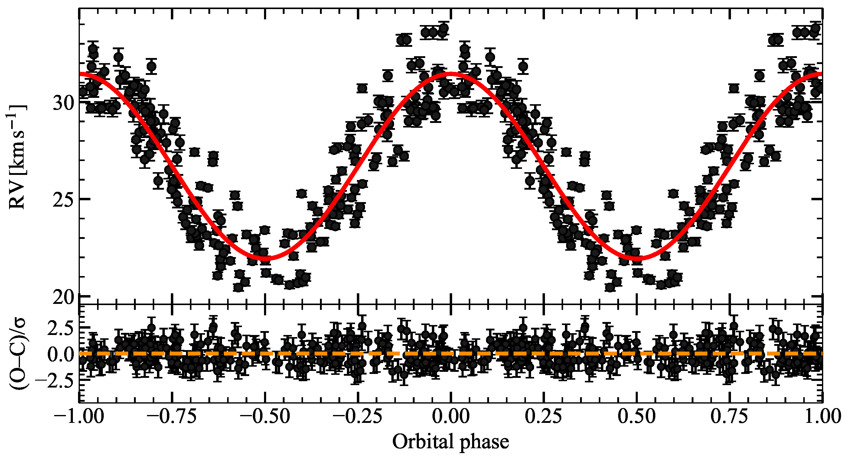
Parameters listed are as follows (line number): 1—orbital period, 2—periastron epoch ($T_0$ given as $T_0-2,400,000$), 3—eccentricity, 4—argument of the periastron, 5—systemic velocity, 6—semi-amplitude of the RV variation of the visible component, 7—mass function, and 8—number of spectra used in the orbit calculation.

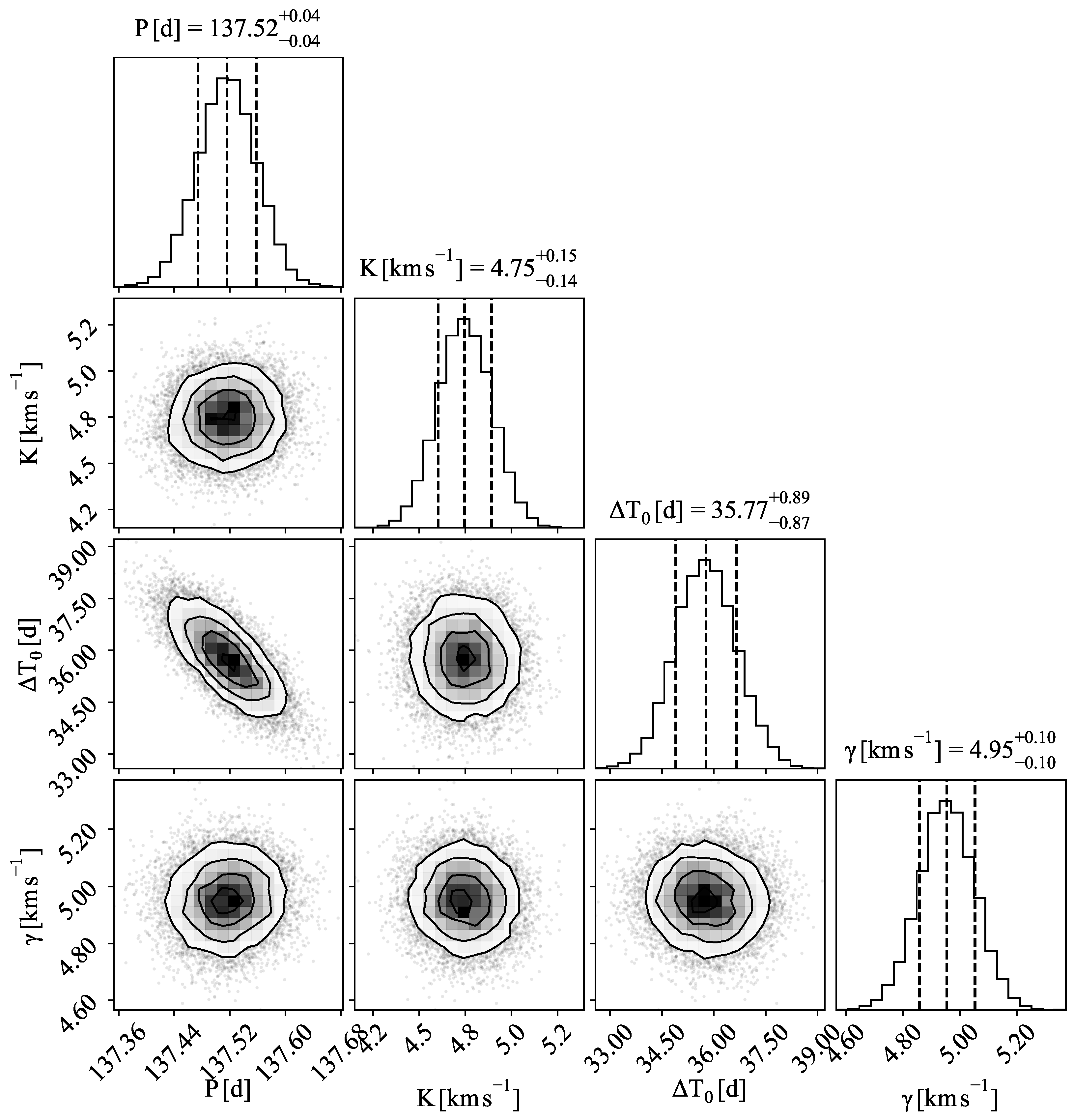
; the phase-folded RV curve and the normalised residuals are shown in Figure 1. While the corresponding corner plot of the posterior distributions is presented in the Figure 2.

5.2. Mizar B

An eccentric six-parameter Keplerian fit to the $N=155$ RV points of Mizar B yields an excellent solution with ${\chi }^2=28.8$ for 149 degrees of freedom (${\chi }_{\nu }^2=0.19$). The full set of orbital elements with 1 $\sigma$ uncertainties is listed in

Table 3. Orbital parameters of Mizar B.

Parameter	[21]	[11]	Our Data
$P_{\mathrm{orb}}$ (days)	175.55 ± 0.05	175.11 ± 0.10	175.06 ± 0.04
$T_0$	37,294.4 ± 1.6	58,175.2 ± 0.7	58,175.9 ± 0.4
e	0.46 ± 0.03	0.56 ±0.09	0.56 ± 0.02
$\omega$ (degrees)	4.3 ± 5.2	353.0 ± 4.6	353.1 ± 4.1
$\gamma$ (km $s^{-1}$)	$-9.30\pm 0.20$	$-14.34\pm 0.04$	−14.33 ± 0.12
K (km $s^{-1}$)	6.30 ± 0.20	6.46 ± 0.53	6.42 ± 0.15
$f\left(m\right)$, $M_{\odot }$	0.0032 ± 0.0005	0.0028 ± 0.0011	0.0083 ± 0.0007
N	89	155	155

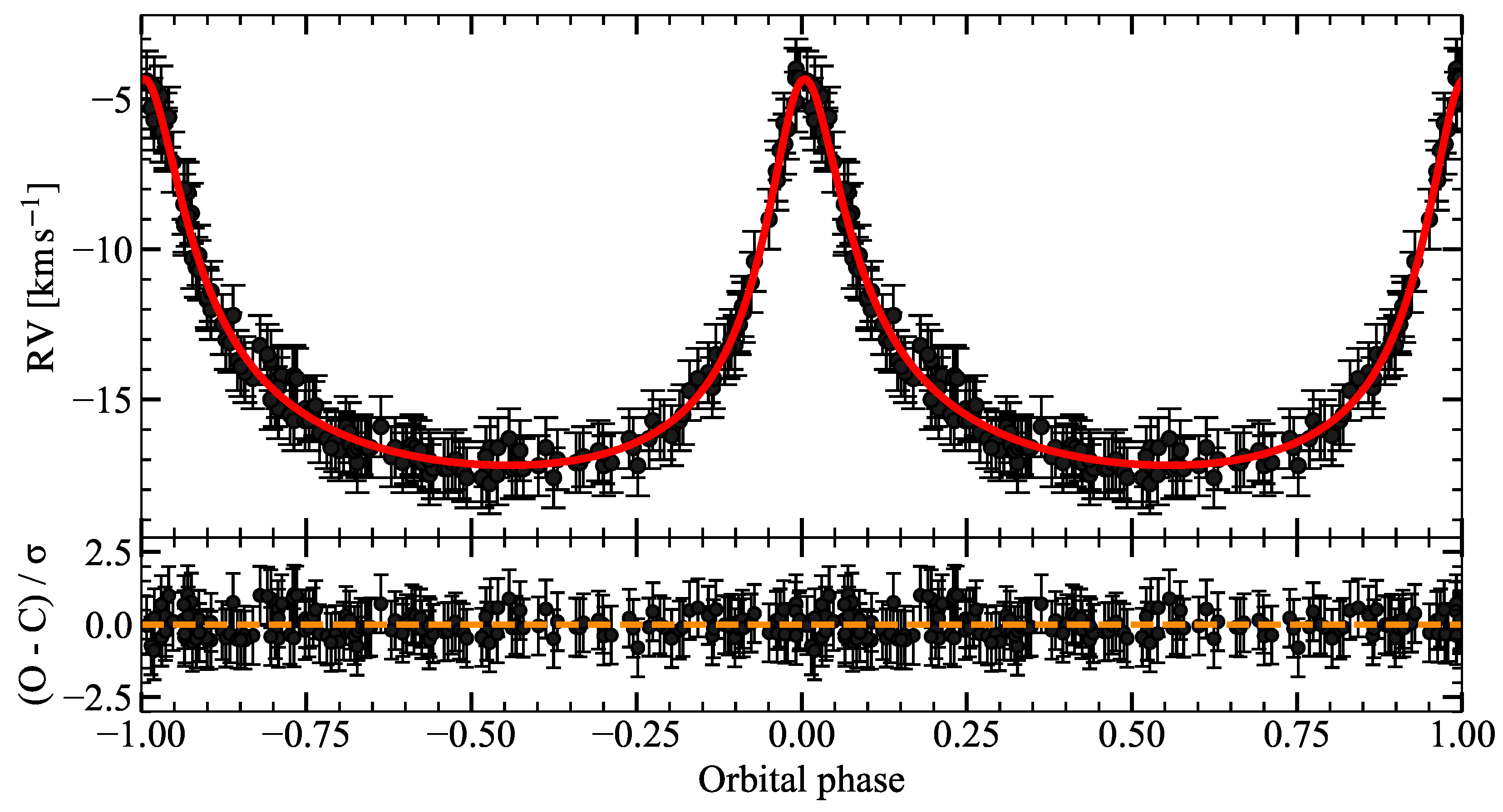
The parameters are the same as in Table 2.

; the phase-folded RV curve and residuals are shown in Figure 3.

5.3. $\nu$ Gem

A circular four-parameter Keplerian fit to the $N=224$ RV measurements of $\nu$ Gem yields a satisfactory solution with ${\chi }^2=246.1$ for 220 degrees of freedom (${\chi }_{\nu }^2=1.12$). The eccentricity is consistent with zero within $2\sigma$, so we fixed $e=0$ and omitted $\omega$ from the fit. The complete set of orbital elements with 1 $\sigma$ uncertainties is given in

Table 4. Orbital parameters of $\nu$ Gem.

Parameter	[24]	[25]	Our Data
$P_{\mathrm{orb}}$ (days)	53.761 ± 0.003	53.770 ± 0.004	53.775 ± 0.003
$T_0$	51,006.60 ± 0.01	58,417.97 ± 0.05	56,656.86 ± 0.02
e	0.079 ± 0.007	0	0
$\omega$ (degrees)	146.2 ± 4.5	-	-
$\gamma$ (km $s^{-1}$)	$-27.63\pm 0.63$	31.51 ± 0.16	31.21 ± 0.05
$K_1$ (km $s^{-1}$)	48.50 ± 1.60	34.68 ± 0.25	29.16 ± 0.16
$f\left(m\right)$, $M_{\odot }$	0.640 ± 0.060	0.229 ± 0.005	0.138 ± 0.002
N	145	261	260

The parameters are the same as in Table 2.

; the phase-folded RV curve and residuals are shown in Figure 4.

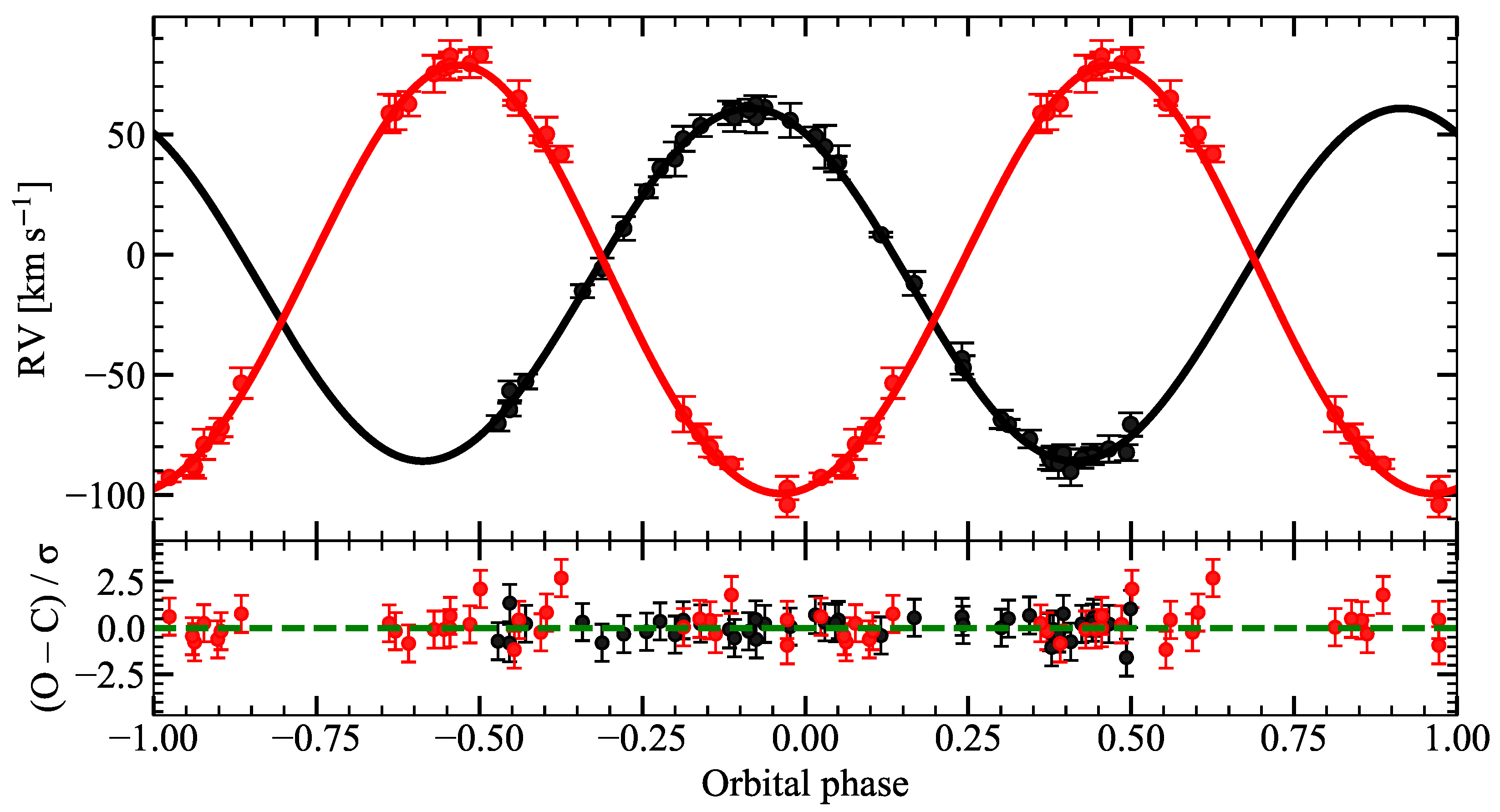
5.4. 2 Lac

A circular four-parameter Keplerian fit to the $N=42$ RV measurements of the primary component of 2 Lac yields ${\chi }^2=33.4$ for 38 degrees of freedom (${\chi }_{\nu }^2=0.88$). A second circular solution for the secondary component, based on $N=28$ points, gives ${\chi }^2=22.2$ for 24 degrees of freedom (${\chi }_{\nu }^2=0.93$). The full set of orbital elements with 1$\sigma$ credible intervals is presented in

Table 5. Orbital parameters of 2 Lac.

Parameter	[27]	[11]	Our Data
$P_{\mathrm{orb}}$ (days)	2.616430 ± 0.000003	2.61654 ± 0.00004	2.61656 ± 0.00002
$T_0$	27,700.800 ± 0.180	59,423.713 ± 0.003	59,021.391 ± 0.002
e	0.04 ± 0.02	0	0
$\omega$ (degrees)	97.4 ± 25.3	-	-
$\gamma$ (km $s^{-1}$)	$-8.90\pm 1.10$	$-13.23\pm 0.34$	$-13.19\pm 0.19$
$K_1$ (km $s^{-1}$)	79.50 ± 1.80	73.19 ± 0.47	73.65 ± 0.31
$K_2$ (km $s^{-1}$)	100.00 ± 1.80	90.25 ± 0.71	89.11 ± 0.34
$f\left(m_1\right)$, $M_{\odot }$	0.137 ± 0.010	0.106 ± 0.002	0.109 ± 0.002
$f\left(m_2\right)$, $M_{\odot }$	0.272 ± 0.015	0.199 ± 0.004	0.201 ± 0.003
N	82/61	42/29	42/29

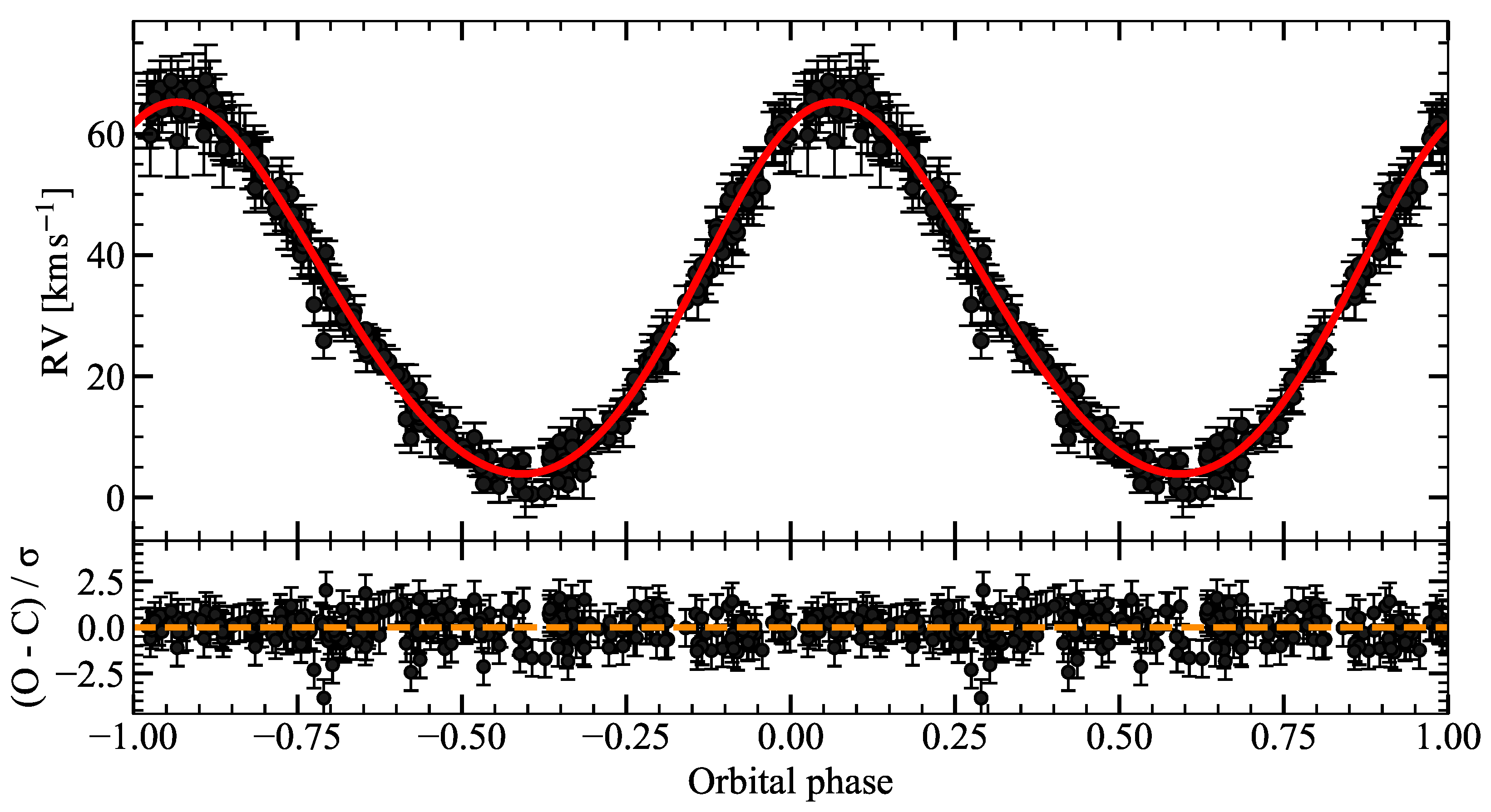
Parameters in the upper 5 lines are the same as in Table 2. The RV semi–amplitudes $K_1$ and $K_2$ as well as the mass functions $f\left(m_1\right)$ and $f\left(m_2\right)$ are listed for the primary and secondary components, respectively. The final row gives N, the number of spectra used for the primary and secondary star (primary/secondary).

; the phase-folded RV curves and the corresponding normalised residuals for both components are displayed in Figure 5.

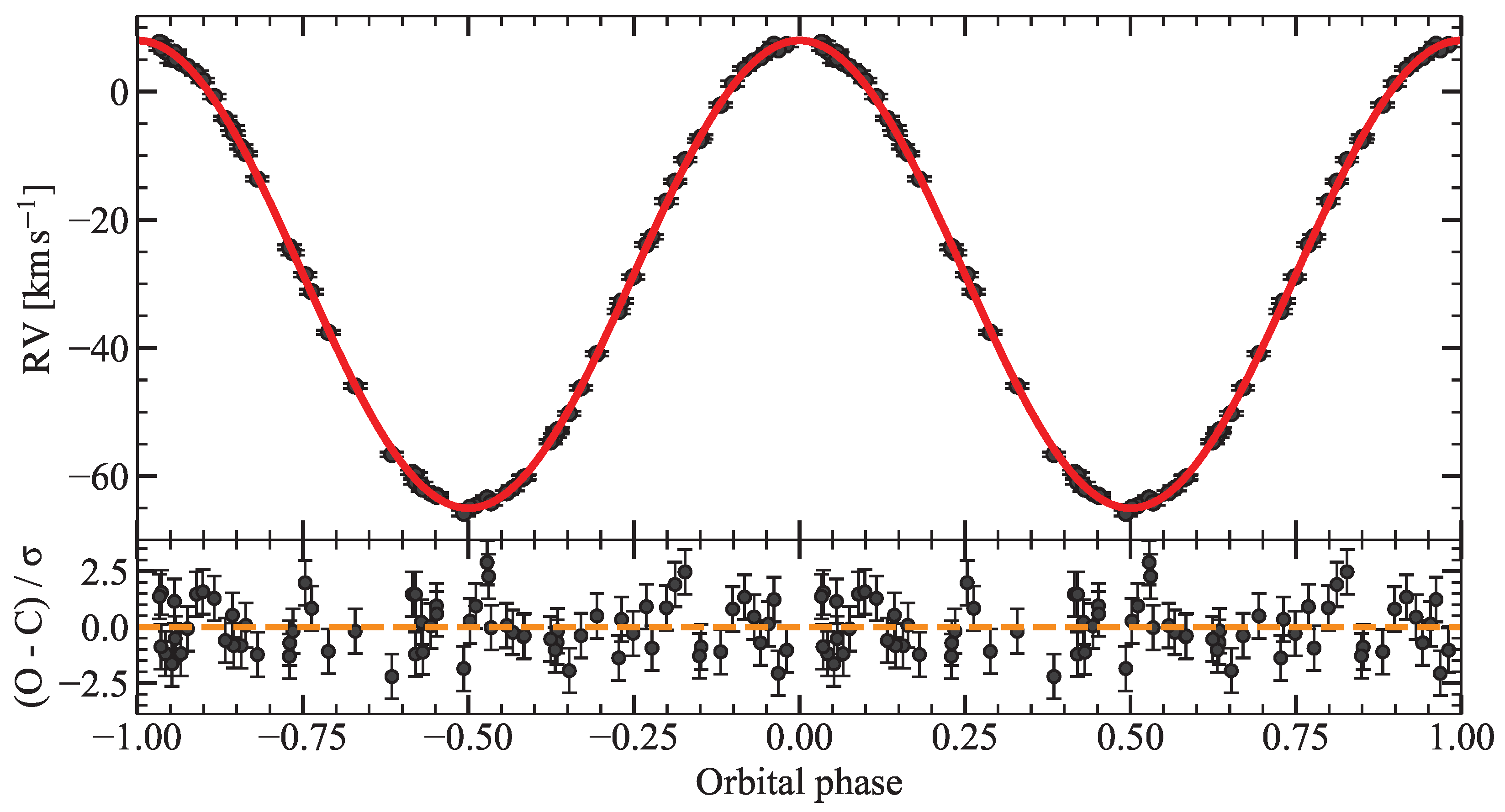
5.5. $\varphi$ Aql

A circular four-parameter Keplerian fit to the $N=70$ RV measurements of $\varphi$ Aql yields ${\chi }^2=95.7$ for 66 degrees of freedom (${\chi }_{\nu }^2=1.45$). The full set of orbital elements with 1$\sigma$ uncertainties is listed in

Table 6. Orbital parameters of $\varphi$ Aql.

Parameter	[30]	[11]	Our Data
$P_{\mathrm{orb}}$ (days)	3.320 ± 0.001	3.320669 ± 0.00002	3.32067 ± 0.00001
$T_0$	23,324.045	59,445.092 ± 0.001	59,027.518 ± 0.001
e	0.06 ± 0.02	0	0
$\omega$ (degrees)	56.0	-	-
$\gamma$ (km $s^{-1}$)	$-27.63\pm 0.63$	$-28.52\pm 0.05$	−28.51 ± 0.03
K (km $s^{-1}$)	38.25 ± 0.72	36.48 ± 0.07	36.50 ± 0.02
$f\left(m\right)$, $M_{\odot }$	0.019 ± 0.001	0.0167 ± 0.0001	0.0167 ± 0.0001
N	34	80	70

The parameters are the same as in Table 2.

; the phase-folded RV curve and the corresponding normalised residuals are displayed in Figure 6.

5.6. Comparison with Previous Work

Across all five systems our posterior medians for P, K, $\gamma$ (and e where fitted) agree with recent literature within the quoted uncertainties; the small residual offsets arise from methodology rather than astrophysical change. Specifically, we (i) enforce a common RV zero-point and barycentric convention, (ii) extract RVs from narrow emission-free windows to suppress wind/disk contamination and SB2 blends, (iii) model SB2s jointly with a shared $\gamma$, and (iv) marginalise over an additive jitter term. These choices reduce known biases that can inflate K or shift $\gamma$ in heterogeneous reductions and chiefly improve precision. Differences in epochs are purely reference-cycle choices ($T_0\to T_0+nP$). Sensitivity tests (broader priors and a fixed-P run) change K and $\gamma$ by $\lesssim 0.5\%$ and $\lesssim 0.02\mathrm{km}{\mathrm{s}}^{-1}$, with $\left|\Delta \mathrm{BIC}\right|<2$ (aside from the fixed-P case, which inflates the formal error on K by construction), confirming likelihood-dominated posteriors.

6. Conclusions

We have presented a uniform Bayesian re-analysis of five bright spectroscopic binaries—Mizar B, 3 Pup, $\nu$ Gem, 2 Lac, and $\varphi$ Aql—based on medium-resolution ($R\simeq 12,000$) spectra obtained with the Three College Observatory 0.81-m telescope between 2015 and 2024. Our workflow combines a Lomb–Scargle period search with an affine-invariant MCMC sampler, explicitly includes an additive jitter term, and reports posterior medians with 16th/84th-percentile credible intervals for every orbital parameter.

1.

For every star the Keplerian model, augmented by a data-driven jitter term, yields ${\chi }_{\nu }^2\approx 1$, indicating that the quoted uncertainties capture the full (instrumental + astrophysical) scatter.

2.

Circular solutions are confirmed for 3 Pup and $\varphi$ Aql, whereas Mizar B, $\nu$ Gem, and 2 Lac require non-zero eccentricities; the posteriors are unimodal and well converged according to both the integrated autocorrelation time and the Gelman–Rubin statistic.

3.

Improvement over earlier work. Relative to the most recent literature values we (i) reduce the semi-amplitude errors from $0.45$–$0.80$ to $0.15$–$0.31$ km $s^{-1}$ (a factor of 2–5), (ii) tighten the systemic velocities to $\pm 0.03$–$0.12$ km $s^{-1}$, (iii) shrink the mass-function uncertainties by $\sim 3\times$, and (iv) lower the 2$\sigma$ upper limit on the eccentricity of 3 Pup from $0.17$ to $0.01$, firmly establishing full circularisation. These gains arise from the homogeneous data set and the full propagation of parameter covariances in the Bayesian framework.

4.

All reduced spectra, radial-velocity measurements, and the Python notebooks that generate the MCMC chains are openly available in our GitHub repository, ensuring full reproducibility.

This study demonstrates that probabilistic modelling, even at moderate spectral resolution, yields reliable orbital parameters with transparent uncertainty budgets. The tighter solutions already open clear avenues for follow-up work:

• The factor-of-2–5 reduction in the uncertainties of K and $\gamma$ lowers the mass-function errors to $\lesssim 10\%$, providing a firmer basis for dynamical-mass estimates once the next Gaia parallaxes become available.
• In the SB2 system 2 Lac the improved semi-amplitudes pin down the mass ratio to $q=0.83\pm 0.01$, a precision sufficient to confront single-star evolutionary tracks and test internal-mixing prescriptions.
• The sub-millipercent period error of $\varphi$ Aql confines predicted eclipse windows to $\pm 30$ min for the next decade, enabling targeted photometry to verify the suspected grazing events.
• For $\nu$ Gem the refined mass ratio and systemic velocity set accurate boundary conditions for planned long-baseline interferometry of its hierarchical triple architecture.
• A common, sub-0.1 km $s^{-1}$ zero-point for $\gamma$ across all five binaries establishes a stable reference frame for long-term radial-velocity monitoring and for combining these data with measurements from other instruments.

These refinements yield reliably characterised orbits, providing accurate inputs for future spectroscopic, interferometric, and photometric studies and tightening empirical constraints on binary evolution and compact-object progenitors.

References

- Torres, G.; Andersen, J.; Giménez, A. Accurate masses and radii of normal stars: Modern results and applications. Astron. Astrophys. Rev. 2010, 18, 67–126. [Google Scholar] [CrossRef]
- Sana, H.; de Mink, S.E.; de Koter, A.; Langer, N.; Evans, C.J.; Gieles, M.; Gosset, E.; Izzard, R.G.; Le Bouquin, J.B.; Schneider, F.R.N. Binary Interaction Dominates the Evolution of Massive Stars. Science 2012, 337, 444. [Google Scholar] [CrossRef]
- Abac, A.G.; Abbott, R.; Abe, H.; Acernese, F.; Ackley, K.; Adamcewicz, C.; Adhicary, S.; Adhikari, N.; Adhikari, R.X.; Adkins, V.K.; et al. Search for Eccentric Black Hole Coalescences during the Third Observing Run of LIGO and Virgo. Astrophys. J. 2024, 973, 132. [Google Scholar] [CrossRef]
- Moe, M.; Di Stefano, R. Mind Your Ps and Qs: The Interrelation between Period (P) and Mass-ratio (Q) Distributions of Binary Stars. Astrophys. J. Suppl. Ser. 2017, 230, 15. [Google Scholar] [CrossRef]
- Lucy, L.B.; Sweeney, M.A. Spectroscopic binaries with circular orbits. Astron. J. 1971, 76, 544–556. [Google Scholar] [CrossRef]
- Foreman-Mackey, D.; Hogg, D.W.; Lang, D.; Goodman, J. emcee: The MCMC Hammer. Publ. Astron. Soc. Pac. 2013, 125, 306. [Google Scholar] [CrossRef]
- Hogg, D.W.; Foreman-Mackey, D. Data Analysis Recipes: Using Markov Chain Monte Carlo. Astrophys. J. Suppl. Ser. 2018, 236, 11. [Google Scholar] [CrossRef]
- Nurmakhametova, S.T.; Vaidman, N.L.; Miroshnichenko, A.S.; Khokhlov, A.A.; Agishev, A.T.; Yermekbayev, B.S.; Danford, S.; Aarnio, A.N. HR 4049: A Spectroscopic Analysis of a Post-AGB Object. Galaxies 2025, 13, 26. [Google Scholar] [CrossRef]
- Vaidman, N.L.; Miroshnichenko, A.S.; Zharikov, S.V.; Khokhlov, S.A.; Agishev, A.T.; Yermekbayev, B.S. Fundamental Parameters and Evolutionary Scenario of HD 327083. Galaxies 2025, 13, 47. [Google Scholar] [CrossRef]
- Ford, E.B. Adaptive Scheduling Algorithms for Planet Searches. Astron. J. 2008, 135, 1008–1020. [Google Scholar] [CrossRef]
- Miroshnichenko, A.S.; Danford, S.; Andronov, I.L.; Aarnio, A.N.; Lauer, D.; Buroughs, H. Refining Orbits of Bright Binary Systems. Galaxies 2023, 11, 8. [Google Scholar] [CrossRef]
- Bailer-Jones, C.A.L.; Rybizki, J.; Fouesneau, M.; Demleitner, M.; Andrae, R. Estimating Distances from Parallaxes. V. Geometric and Photogeometric Distances to 1.47 Billion Stars in Gaia Early Data Release 3. Astron. J. 2021, 161, 147. [Google Scholar] [CrossRef]
- Miroshnichenko, A.S.; Danford, S.; Zharikov, S.V.; Klochkova, V.G.; Chentsov, E.L.; Vanbeveren, D.; Zakhozhay, O.V.; Manset, N.; Pogodin, M.A.; Omarov, C.T.; et al. Properties of Galactic B[e] Supergiants. V. 3 Pup-Constraining the Orbital Parameters and Modeling the Circumstellar Environments. Astrophys. J. 2020, 897, 48. [Google Scholar] [CrossRef]
- Nodyarov, A.S.; Miroshnichenko, A.S.; Khokhlov, S.A.; Zharikov, S.V.; Manset, N.; Klochkova, V.G.; Grankin, K.N.; Arkharov, A.A.; Efimova, N.; Klimanov, S.; et al. Toward Understanding the B[e] Phenomenon. IX. Nature and Binarity of MWC645. Astrophys. J. 2022, 936, 129. [Google Scholar] [CrossRef]
- Miroshnichenko, A.S.; Zharikov, S.V.; Korčaková, D.; Manset, N.; Mennickent, R.; Khokhlov, S.A.; Danford, S.; Raj, A.; Zakhozhay, O.V. Binarity among objects with the Be and B[e] phenomena. Contrib. Astron. Obs. Skaln. Pleso 2020, 50, 513–517. [Google Scholar] [CrossRef]
- Khokhlov, S.A.; Miroshnichenko, A.S.; Zharikov, S.V.; Grankin, K.N.; Zakhozhay, O.V.; Manset, N.; Arkharov, A.A.; Efimova, N.; Klimanov, S.; Larionov, V.M.; et al. Toward Understanding the B[e] Phenomenon. VIII. Nature and Variability of IRAS 07080+0605. Astrophys. J. 2022, 932, 36. [Google Scholar] [CrossRef]
- Rovero, A.C.; Ringuelet, A.E. 3 Puppis : A peculiar object with infrared excess. Mon. Not. R. Astron. Soc. 1994, 266, 203–211. [Google Scholar] [CrossRef]
- Meilland, A.; Kanaan, S.; Fernandes, M.B.; Chesneau, O.; Millour, F.; Stee, P.; Lopez, B. Resolving the dusty circumstellar environment of the A[e] supergiant HD 62623 with the VLTI/MIDI. In Active OB Stars: Structure, Evolution, Mass-Loss, and Critical Limits; Neiner, C., Wade, G., Meynet, G., Peters, G., Eds.; IAU Symposium; Cambridge University Press: Cambridge, UK, 2011; Volume 272, pp. 406–407. [Google Scholar] [CrossRef]
- Kraus, M.; Oksala, M.E.; Cidale, L.S.; Arias, M.L.; Torres, A.F.; Borges Fernandes, M. Discovery of SiO Band Emission from Galactic B[e] Supergiants. Astrophys. J. Lett. 2015, 800, L20. [Google Scholar] [CrossRef]
- Abt, H.A.; Levy, S.G. Improved study of metallic-line binaries. Astrophys. J. Suppl. Ser. 1985, 59, 229–247. [Google Scholar] [CrossRef]
- Gutmann, F. The spectroscopic orbit of Ursae Majoris (Mizar B). Publ. Dom. Astrophys. Obs. Vic. 1965, 12, 361–371. [Google Scholar]
- Cannon, A.J.; Pickering, E.C. Henry Draper Catalogue and Extension (HD, HDE); VizieR Online Data Catalog: III/135A; Centre de Données astronomiques de Strasbourg (CDS): Strasbourg, France, 1993; Available online: https://vizier.cds.unistra.fr/viz-bin/cat/III/135A (accessed on 25 August 2025).
- Gardner, T.; Monnier, J.D.; Fekel, F.C.; Schaefer, G.; Johnson, K.J.C.; Le Bouquin, J.B.; Kraus, S.; Anugu, N.; Setterholm, B.R.; Labdon, A.; et al. ARMADA. I. Triple Companions Detected in B-type Binaries α Del and ν Gem. Astron. J. 2021, 161, 40. [Google Scholar] [CrossRef]
- Klement, R.; Hadrava, P.; Rivinius, T.; Baade, D.; Cabezas, M.; Heida, M.; Schaefer, G.H.; Gardner, T.; Gies, D.R.; Anugu, N.; et al. ν Gem: A Hierarchical Triple System with an Outer Be Star. Astrophys. J. 2021, 916, 24. [Google Scholar] [CrossRef]
- Miroshnichenko, A.S.; Chari, R.; Danford, S.; Prendergast, P.; Aarnio, A.N.; Andronov, I.L.; Chinarova, L.L.; Lytle, A.; Amantayeva, A.; Gabitova, I.A.; et al. Searching for Phase-Locked Variations of the Emission-Line Profiles in Binary Be Stars. Galaxies 2023, 11, 83. [Google Scholar] [CrossRef]
- Zorec, J.; Royer, F. Rotational velocities of A-type stars. IV. Evolution of rotational velocities. Astron. Astrophys. 2012, 537, A120. [Google Scholar] [CrossRef]
- Hilditch, R.W. The binary systems 14 Cephei and 2 Lacertae. Mon. Not. R. Astron. Soc. 1974, 169, 323–329. [Google Scholar] [CrossRef]
- Eggleton, P.P.; Tokovinin, A.A. A catalogue of multiplicity among bright stellar systems. Mon. Not. R. Astron. Soc. 2008, 389, 869–879. [Google Scholar] [CrossRef]
- Cowley, A.; Cowley, C.; Jaschek, M.; Jaschek, C. A study of the bright A stars. I. A catalogue of spectral classifications. Astron. J. 1969, 74, 375–406. [Google Scholar] [CrossRef]
- Harper, W. The Orbit of the Spectroscopic Binary phi Aquilae. Publ. Dom. Astrophys. Obs. Vic. 1922, 2, 179–182. [Google Scholar]
- Soubiran, C.; Le Campion, J.F.; Cayrel de Strobel, G.; Caillo, A. The PASTEL catalogue of stellar parameters. Astron. Astrophys. 2010, 515, A111. [Google Scholar] [CrossRef]
- Scargle, J.D. Studies in astronomical time series analysis. II. Statistical aspects of spectral analysis of unevenly spaced data. Astrophys. J. 1982, 263, 835–853. [Google Scholar] [CrossRef]
- VanderPlas, J.T. Understanding the Lomb-Scargle Periodogram. Astrophys. J. Suppl. Ser. 2018, 236, 16. [Google Scholar] [CrossRef]
- Hilditch, R.W. An Introduction to Close Binary Stars; Cambridge University Press: Cambridge, UK, 2001. [Google Scholar]
- Wright, J.T.; Howard, A.W. Efficient Fitting of Multiplanet Keplerian Models to Radial Velocity and Astrometry Data. Astrophys. J. Suppl. Ser. 2009, 182, 205–215. [Google Scholar] [CrossRef]
- Metropolis, N.; Rosenbluth, A.W.; Rosenbluth, M.N.; Teller, A.H.; Teller, E. Equation of State Calculations by Fast Computing Machines. J. Chem. Phys. 1953, 21, 1087–1092. [Google Scholar] [CrossRef]
- Hastings, W.K. Monte Carlo Sampling Methods using Markov Chains and their Applications. Biometrika 1970, 57, 97–109. [Google Scholar] [CrossRef]
- Goodman, J.; Weare, J. Ensemble samplers with affine invariance. Commun. Appl. Math. Comput. Sci. 2010, 5, 65–80. [Google Scholar] [CrossRef]
- Zechmeister, M.; Kürster, M. The generalised Lomb-Scargle periodogram. A new formalism for the floating-mean and Keplerian periodograms. Astron. Astrophys. 2009, 496, 577–584. [Google Scholar] [CrossRef]
- Wright, J.T. Radial Velocity Jitter in Stars from the California and Carnegie Planet Search at Keck Observatory. Publ. Astron. Soc. Pac. 2005, 117, 657–664. [Google Scholar] [CrossRef]
- Zechmeister, M.; Reiners, A.; Amado, P.J.; Azzaro, M.; Bauer, F.F.; Béjar, V.J.S.; Caballero, J.A.; Guenther, E.W.; Hagen, H.J.; Jeffers, S.V.; et al. Spectrum radial velocity analyser (SERVAL). High-precision radial velocities and two alternative spectral indicators. Astron. Astrophys. 2018, 609, A12. [Google Scholar] [CrossRef]
- Harris, C.R.; Millman, K.J.; van der Walt, S.J.; Gommers, R.; Virtanen, P.; Cournapeau, D.; Wieser, E.; Taylor, J.; Berg, S.; Smith, N.J.; et al. Array programming with NumPy. Nature 2020, 585, 357–362. [Google Scholar] [CrossRef] [PubMed]
- Virtanen, P.; Gommers, R.; Oliphant, T.E.; Haberland, M.; Reddy, T.; Cournapeau, D.; Burovski, E.; Peterson, P.; Weckesser, W.; Bright, J.; et al. SciPy 1.0: Fundamental algorithms for scientific computing in Python. Nat. Methods 2020, 17, 261–272. [Google Scholar] [CrossRef] [PubMed]
- The Pandas Development Team. pandas-Dev/Pandas: Pandas (v2.3.0); Zenodo: Geneva, Switzerland, 2025. [Google Scholar] [CrossRef]
- Hunter, J.D. Matplotlib: A 2D Graphics Environment. Comput. Sci. Eng. 2007, 9, 90–95. [Google Scholar] [CrossRef]
- Foreman-Mackey, D. corner.py: Scatterplot matrices in Python. J. Open Source Softw. 2016, 1, 24. [Google Scholar] [CrossRef]
- Miroshnichenko, A.S.; Zharikov, S.V.; Manset, N.; Khokhlov, S.A.; Nodyarov, A.S.; Klochkova, V.G.; Danford, S.; Kuratova, A.K.; Mennickent, R.; Chojnowski, S.D.; et al. Recent Progress in Finding Binary Systems with the B[e] Phenomenon. Galaxies 2023, 11, 36. [Google Scholar] [CrossRef]
- Johnson, H.L.; Neubauer, F.J. Spectrographic Orbits of Two c Stars: μ Persei and 13 Puppis. Publ. Astron. Soc. Pac. 1946, 58, 248. [Google Scholar] [CrossRef]