Abstract
Resolved spectroscopic binaries (RSBs) are an extremely valuable class of objects, being the only (apart from trigonometric) supplier of dynamical stellar parallaxes. This circumstance, as well as the comparative paucity of studied RSBs, makes the problem of identifying binary systems potentially capable of being added to the list of known RSBs extremely urgent. In this paper, we propose a methodology for estimating the probability of a spectroscopic binary system to be resolved into components, perform the first step of its application to the SB9 catalogue, and present preliminary results, in particular, a list of the most promising RSB candidates.
1. Introduction
A significant fraction of stars in the Milky Way are binary or multiple stars. The studies conducted in [1,2,3,4,5] allow us to conclude that F-G-K-M stars may have an observed binary fraction of 20–40%, while that of O- and B-type stars may reach 100%.
A very interesting observational class of binary systems is resolved spectroscopic binaries (RSBs). Like some other observational classes (for example, double-lined eclipsing binaries, DLEBs), they are suppliers of dynamic stellar masses and other component parameters, but, most importantly, they provide us with the only way (apart from trigonometric parallax) to directly determine (rather than estimate) the distances to stars. Ref. [6] was one of the first to draw attention to this fact and compiled a list of about forty RSB systems. Later, Refs. [7,8,9,10] presented more representative lists, and, finally, Ref. [11] recently published a catalogue containing presumably all RSB systems studied to date. The catalogue in [11] is the most comprehensive list of RSBs to date, and it contains orbital elements (the orbital period P (yr), time of periastron (JD), eccentricity e, inclination of the orbital plane i (deg), position angle of the ascending node (deg), periastron longitude (deg), semi-major axis a (mas), and semi-major axis a (AU)), masses, orbital and trigonometric parallaxes, spectral classification, multicolour photometry, and reddening for 173 objects.
The exceptional importance of this class of binary systems makes the task of discovering new RSBs extremely urgent. One of the possibilities of replenishing the list of known RSBs is an astrometric study of the most “promising” (primarily the widest) spectroscopic binaries with lines of both components in the spectrum (so-called SB2). The results of such a study were presented, for example, in [12].
Currently, the most complete and constantly updated catalogue of spectroscopic binaries is presented in [13] (hereafter, SB9). In this paper, we focus on estimating the probability of the astrometric resolution of spectroscopic binaries into components. We develop an original methodology for estimating this probability and conduct a pilot application of it to the SB9 catalogue. This paper is structured as follows: The methodology for estimating the resolution probability function of spectroscopic binary stars is described in Section 2. Results are presented and discussed in Section 3. Finally, in Section 4, we draw our conclusions.
2. Methodology for Estimating the Resolution Probability Function of Spectroscopic Binary Stars
Suppose that, in order for an unresolved spectroscopic binary star (SB) to be spatially resolved (RSB), it must have parameter values characteristic of other resolved spectroscopic binaries, i.e., be close to them in some parameter space. We also assume that the parameter space, for which the first assumption is correct, is formed by the observational parameters of the spectroscopic binaries, defined in the Catalogue of Resolved Spectroscopic Binaries [14] (hereafter, RSBcat) and the SB9 catalogue [13], which can be found in Table 1. The subset of SB9 objects identified with [14] is denoted by SB9R (), and the subset not identified with [14] (i.e., unresolved) is denoted by SB9U. Note that , as 24 of the 173 RSBcat objects are not included in the SB9 catalogue. Accordingly, the set of all catalogue objects is SB9A (). Note also that we consider only double-lined spectroscopic binary (SB2) systems from the SB9 catalogue, as only those systems can be fully solved for the orbital parameters (and thus the orbital parallax).

Table 1.
Parameters of spectroscopic binary stars in the RSBcat and SB9 catalogues. (*) The values of these parameters were added from the SIMBAD database for stars in the RSBcat and SB9 catalogues.
The essence of the proposed method is extremely simple: to use multidimensional distances in the space of observational parameters given a unified scale to estimate the proximity of spectroscopic binaries from SB9U and SB9R and, on the basis of the value of the obtained parametric distances, to estimate the prospectivity of the observations of objects from SB9U in terms of the probability of being resolved. We denote by the ordered set of SB9R object parameters, and we denote by the same set of SB9U object parameters. From the parameters given in Table 1, we choose the following values to estimate the parametric distances: , e, , , , , , , , , , , , , . Hereafter, k is the number of the parameter (component of the parametric vector).
Here, we use the vector notation to illustrate the idea of the method, but, of course, the quantities compiled in this way are not true vectors. Since all observational parameters have distinct scales of values, it is first necessary to renormalise all components , to the domain of values of the corresponding parameters for all SB9A objects and bring them to a unit value interval to equilibrate all parameters with each other. For the purpose of demonstrating the method, we assume that all parameters are equally important and have the same weight while realising that this assumption can be false in some other cases, and the unequal weighting of the parameters can be easily accounted for by normalising the components differently. In order to renormalise and , at first, we have to calculate the bounding box in the parameter space that would contain both SB9U and SB9R sets of objects. Hereafter, we imply that every i-th object in SB9R and every j-th object in SB9U have their own and values, so omitting i and j object indices means that the expression is applicable for all objects.
The lower bound is determined by the expression
where i is the number of the object in the SB9R set, and j is the number of the object in the SB9U set. The upper bound is determined accordingly by the expression
Given that is the range of values of the k-th parameter, we finally obtain the expression for the renormalised parameters:
In the following, we omit the notation of the dimensionless value (~) and assume that all components of vectors and are already renormalised.
The mean values of and point to the centres of the sets of objects SB9R and SB9U, respectively, in the observation parameter space. The vector defines the principal direction in the parameter space between the SB9U and SB9R sets.
When calculating the mean vectors and , one has to take into account that, for every k-th parameter, there may be different numbers of objects for whom this parameter is measured and known from SB9cat. Therefore, the definition of the mean vectors can be written as follows:
Also, for the principal direction vector , we have
and normalising this vector gives the weights indicating the significance of the parameters with regard to the difference between the SB9U and SB9R sets.
Values for the principal direction vector components are provided in Table 2 in the “SB9U-SB9R mean diff.” and “Normalised mean diff.” columns.
Table 2.
Properties of the parameter distributions of spectroscopic binary stars from SB9R and SB9U sets.
The proximity of the SB9U object to the SB9R region is determined by the distance . The most interesting measure of parametric proximity is the distance to the nearest SB9R object, , since its evaluation allows us to directly generate a list of candidates from SB9U to RSB and point to specific comparison objects. The smaller the and of an object from SB9U, the higher the probability that it can be resolved. Thus, for each SB9U object, we have a proximity criterion for the whole SB9R set () and for an individual SB9R object ().
When calculating the parametric distances and , it should be taken into account that, for angular components, their arithmetic difference will not be the minimum angle difference, required for distance estimation, and the corresponding summands in the norm calculation should be calculated as . In addition, it should be considered that, since the values of all parameters are not known simultaneously for all objects, for each object from SB9U or a pair of objects from SB9U and SB9R, when computing and , the expression for the norm vector will only include the of the known parameter values out of the total number of parameters. Hence, the resulting value of and is not distorted downward when due to the use of fewer identically normalised components, i.e., so that the parametric distance between the objects does not become formally smaller just because fewer parameters are known about them from observations, and the values of , must be corrected by the factor .
With all these considerations, we can rewrite and in a more detailed form. First, we define an absolute minimum difference between the k-th components as the function:
Then, the parametric distance between two objects is just an Euclidean distance corrected for undefined quantities:
Then, the distance to the SB9R set centre for the j-th SB9U object is simply
and the distance to the nearest SB9R object for the j-th SB9U object is
where m is the number of an SB9R object that has minimal distance l to the j-th SB9U object
3. Results and Discussion
An analysis of the distribution of observational parameters for the SB9U and SB9R sets shows that SB9R includes, on average, brighter stars with a larger orbital period and eccentricity and, correspondingly, smaller amplitudes of radial velocities. The lowest contribution to the difference between SB9R and SB9U is given by the radial velocity of the system , and the difference in the mean parallaxes and radial velocities of the primary component of the binary system is somewhat more significant, but the contribution of all other quantities is approximately the same. The properties of the distributions of the observational parameters are given in Table 2: the columns SB9R (min, max, mean, stddev) and SB9U (min, max, mean, stddev) are given for SB9R and SB9U, respectively, containing the parameter value interval boundaries, mean values, and their standard deviations; the column “SB9U-SB9R” contains components of the vector , i.e., the difference between the mean values SB9U.mean-SB9R.mean; and the “Normalised mean diff.” column contains the values of the components of the normalised vector to estimate their relative contribution.
As a result of the above methodology, we obtained lists of SB9U objects ordered by the parametric distances and . The most promising objects for observation, corresponding to the smallest values of the parametric distances, are listed in Table 3 and Table 4. Figure 1 (red points) shows the location of SB9U objects in coordinates. For comparison, the figure also shows the position of SB9R objects (red crosses).
Table 3.
The most promising SB9U systems in terms of parametric distance to the mean value in the SB9R (to the centre of the SB9R object cloud). The RSBcat HIP column contains the Hipparcos number of the parametrically nearest (by ) SB9R object.
Table 4.
The most promising SB9U systems in terms of the parametric distance to the nearest SB9R object, whose HIP number is given in the RSBcat HIP column.
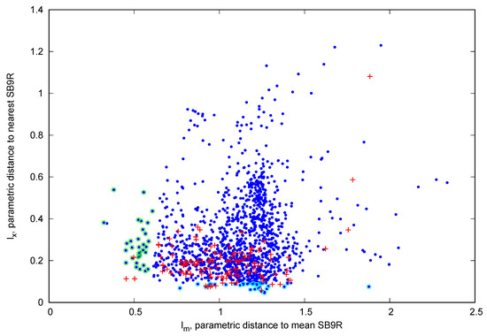
Figure 1.
Parametric distances from the SB9U (blue points) and SB9R (red crosses) objects to the parametric centre (mean position) of the SB9R set () and to its nearest SB9R object (). Circles mark the first 30 objects with the smallest (green) and smallest (cyan) distances.
A complete list of promising candidates is available upon request.
As one can see in Table 3 and Table 4, the smallest values are significantly lower than the smallest values, and both tables have no common objects. At first glance, this looks like an inconsistency in the proposed methodology, as a solid result would have had a single list of objects, but, in fact, this indicates a more complex problem.
The value of represents the distance to the SB9R population average, while the value of represents the distance to the nearest neighbour in SB9R. Both of these measures are valuable but in different ways, and there is no fair reason to prefer one over the other. The distance is more precise, as it reveals what SB9R object is the nearest neighbour to an SB9U object; additionally, since the smallest values of are much lower than the values, these particular SB9U and SB9R objects are parametrically closer than other objects in general, and, for that reason, both should probably be resolved. The distance is a rough measure; the important thing here is not its value for a particular object but rather its range for all SB9R objects, as every SB9U object that falls within that range should probably be resolved. The basic idea behind the values and Table 3 is that the closer to the centre of an SB9R cloud an SB9U object is, the higher the probability of its resolution should be; however, considering the SB9R mean position an optimal parameter combination in terms of binary resolvability is, of course, a gross oversimplification.
Table 3 shows that, for the smallest values, the corresponding values are comparable. This means that, nearer the centre of the SB9R cloud, the population density of SB9U and SB9R is about the same. In comparison, Table 4 shows pretty large values corresponding to the smallest values, and this means that the population density of SB9U is much higher at the edge of the SB9R cloud than at its centre. This difference in population density in the parameter space is the main reason why a single list of best candidate objects cannot be produced within this methodology (at least not now).
If we limit ourselves to a subset of SB9U objects that have , then it is possible for common objects to appear in both tables, but this would be a bad choice since a huge number of better nearest neighbour candidates would drop out. Alternatively, we can explicitly merge tables and sort objects by the value or by the norm of these measures ; either way, such a result would not contain candidates.
Therefore, we propose to use Table 4 as the main list of candidates and Table 3 as a secondary guide and examine these spectroscopic binaries by other means.
It should be remembered that the SB9 catalogue contains orbital solutions rather than spectroscopic systems (multiple solutions are often given for a single spectroscopic system). In total, SB9 contains 5099 entries, of which 339 (7%) are SB9R and 4760 (93%) are SB9U. This means that the number of candidate stars is somewhat smaller than the number of candidate records. In addition, obviously, the probability of a spectroscopic binary to be resolved into components is also affected by other parameters: the angular distance between the components, the brightness of the system, the magnitude difference of the components, the orbit orientation, and so on. However, we believe that the values that we obtained can be used as rough estimates.
It should be added that another promising source of RSB candidates is the LAMOST survey [15,16]. Spectroscopic binary studies using LAMOST are being carried out quite intensively in [17,18,19,20]. This source also deserves the closest attention.
4. Conclusions
Resolved spectroscopic binaries (RSBs) are the only way (besides trigonometric parallax) to determine the dynamical, hypothesis-free distances to the stars of the Galaxy. Today, we know very few (less than two hundred) RSBs, so each new object makes a significant contribution to our knowledge of stellar distances.
We developed a method for estimating the probability of resolving the components of double-lined spectroscopic binaries (SB2), which depends on orbital element values and component parameters. The main points of this work are summarised as follows:
- The probability of the resolution of unresolved objects could be inferred from the similarity to resolved objects;
- Distances in the space of observational parameters could be used as a basic and straightforward measure of similarity;
- The highest similarity is achieved between individual objects, and it is loosely connected to the parameter space occupied by resolved objects.
The method was applied to the principal catalogue of spectroscopic binaries, SB9, and the results of this application are shown in Figure 1 and Table 1. A complete list of promising candidates is available upon request. Obviously, these results will be useful for organising astrometric/interferometric observations of spectroscopic binary systems in order to resolve them into components and add them to the list of resolved spectroscopic binaries.
Author Contributions
All authors contributed to the study conception and design. Material preparation, data collection, and analysis were performed by all authors. The first draft of the manuscript was written by D.B.Z., and all authors commented on previous versions of the manuscript. All authors have read and agreed to the published version of the manuscript.
Funding
A. Sachkov and O. Malkov thank the Foundation for the Advancement of Theoretical Physics and Mathematics “BASIS” for its support, grant No 25-1-1-34-1.
Data Availability Statement
Data are available on request from the authors.
Acknowledgments
We are grateful to the anonymous reviewers whose constructive comments greatly helped us to improve this paper. We warmly thank James Wicker for his invaluable assistance in preparing the manuscript. We thank Space Science and Geospatial Institute, Entoto Observatory and Research Center and Astronomy and Astrophysics Department for supporting this research. This research has made use of the SAO/NASA Astrophysics Data System and the SIMBAD database, operated at CDS, Strasbourg, France.
Conflicts of Interest
The authors have no relevant financial or non-financial interests to disclose.
References
- Duchêne, G.; Kraus, A. Stellar Multiplicity. Annu. Rev. Astron. Astrophys. 2013, 51, 269–310. [Google Scholar] [CrossRef]
- Duquennoy, A.; Mayor, M. Multiplicity among Solar Type Stars in the Solar Neighbourhood—Part Two—Distribution of the Orbital Elements in an Unbiased Sample. Astron. Astrophys. 1991, 248, 485. [Google Scholar]
- Raghavan, D.; McAlister, H.A.; Henry, T.J.; Latham, D.W.; Marcy, G.W.; Mason, B.D.; Gies, D.R.; White, R.J.; ten Brummelaar, T.A. A Survey of Stellar Families: Multiplicity of Solar-type Stars. Astrophys. J. Suppl. Ser. 2010, 190, 1–42. [Google Scholar] [CrossRef]
- Sheikhi, N.; Hasheminia, M.; Khalaj, P.; Haghi, H.; Zonoozi, A.H.; Baumgardt, H. The binary fraction and mass segregation in Alpha Persei open cluster. Mon. Not. R. Astron. Soc. 2016, 457, 1028–1036. [Google Scholar] [CrossRef]
- Yuan, H.; Liu, X.; Xiang, M.; Huang, Y.; Chen, B.; Wu, Y.; Hou, Y.; Zhang, Y. Stellar Loci II. A Model-free Estimate of the Binary Fraction for Field FGK Stars. Astrophys. J. 2015, 799, 135. [Google Scholar] [CrossRef]
- Pourbaix, D. Resolved double-lined spectroscopic binaries: A neglected source of hypothesis-free parallaxes and stellar masses. Astron. Astrophys. Suppl. Ser. 2000, 145, 215–222. [Google Scholar] [CrossRef]
- Anguita-Aguero, J.; Mendez, R.A.; Claveria, R.M.; Costa, E. Orbital Elements and Individual Component Masses from Joint Spectroscopic and Astrometric Data of Double-line Spectroscopic Binaries. Astron. J. 2022, 163, 118. [Google Scholar] [CrossRef]
- Gallenne, A.; Mér, A.; Kervella, P.; Graczyk, D.; Pietrzyński, G.; Gieren, W.; Pilecki, B. The Araucaria project: High-precision orbital parallaxes and masses of binary stars. I. VLTI/GRAVITY observations of ten double-lined spectroscopic binaries. Astron. Astrophys. 2023, 672, A119. [Google Scholar] [CrossRef]
- Jancart, S.; Jorissen, A.; Babusiaux, C.; Pourbaix, D. Astrometric orbits of SB9 stars. Astron. Astrophys. 2005, 442, 365–380. [Google Scholar] [CrossRef]
- Piccotti, L.; Docobo, J.Á.; Carini, R.; Tamazian, V.S.; Brocato, E.; Andrade, M.; Campo, P.P. A study of the physical properties of SB2s with both the visual and spectroscopic orbits. Mon. Not. R. Astron. Soc. 2020, 2, 2709–2721. [Google Scholar] [CrossRef]
- Zeleke, D.B.; Sachkov, A.M.; Malkov, O.Y.; Negu, S.H.; Tessema, S.B.; Grinenko, A.D. Resolved spectroscopic binaries: Orbital elements and parallaxes. Astrophys. Space Sci. 2025, 370, 1. [Google Scholar] [CrossRef]
- Taylor, S.F.; Harvin, J.A.; McAlister, H.A. The CHARA Catalog of Orbital Elements of Spectroscopic Binary Stars. Publ. Astron. Soc. Pac. 2003, 115, 609–617. [Google Scholar] [CrossRef]
- Pourbaix, D.; Tokovinin, A.A.; Batten, A.H.; Fekel, F.C.; Hartkopf, W.I.; Levato, H.; Morrell, N.I.; Torres, G.; Udry, S. The ninth catalogue of spectroscopic binary orbits. Astron. Astrophys. 2004, 424, 727–732. [Google Scholar] [CrossRef]
- Zeleke, D.B.; Pakhomova, P.V.; Tessema, S.B.; Negu, S.H.; Malkov, O.Y. The Catalog of Resolved Spectroscopic Binaries: Development and Description. Astron. Rep. 2023, 67, 576–580. [Google Scholar] [CrossRef]
- Luo, A.; Zhao, Y.; Zhao, G.; Deng, L.; Liu, X.; Jing, Y.; Wang, G.; Zhang, H.; Shi, J.; Cui, X.; et al. The first data release (DR1) of the LAMOST regular survey. Res. Astron. Astrophys. 2015, 15, 1095. [Google Scholar] [CrossRef]
- Luo, A.L.; Zhao, Y.H.; Zhao, G. VizieR Online Data Catalog: LAMOST DR5 catalogs (Luo+, 2019). Vizier Online Data Cat. 2019, 5165, V / 164. [Google Scholar]
- Guo, S.; Kovalev, M.; Li, J.; Lü, G.; Jia, S.; Li, Z.; Li, J.; Xiong, J.; Yang, M.; Han, Z.; et al. Orbital Parameters of 665 Double-lined Spectroscopic Binaries in the LAMOST Medium-Resolution Survey. arXiv 2025, arXiv:2504.11954. [Google Scholar] [CrossRef]
- Jing, Y.; Mao, T.X.; Wang, J.; Liu, C.; Chen, X. Half a Million Binary Stars Identified from the Low-resolution Spectra of LAMOST. Astrophys. J. Suppl. Ser. 2025, 277, 15. [Google Scholar] [CrossRef]
- Liu, J.; Zhang, B.; Wu, J.; Ting, Y.S. Double-lined Spectroscopic Binaries from the LAMOST Low-resolution Survey. Astrophys. J. Suppl. Ser.s 2024, 275, 40. [Google Scholar] [CrossRef]
- Zhao, X.; Wang, S.; Liu, J. Searching for Accreting Compact Binary Systems from Spectroscopy and Photometry: Application to LAMOST Spectra. Astrophys. J. 2025, 984, 9. [Google Scholar] [CrossRef]

Disclaimer/Publisher’s Note: The statements, opinions and data contained in all publications are solely those of the individual author(s) and contributor(s) and not of MDPI and/or the editor(s). MDPI and/or the editor(s) disclaim responsibility for any injury to people or property resulting from any ideas, methods, instructions or products referred to in the content. |
© 2025 by the authors. Licensee MDPI, Basel, Switzerland. This article is an open access article distributed under the terms and conditions of the Creative Commons Attribution (CC BY) license (https://creativecommons.org/licenses/by/4.0/).