1PN Effective Binary Lagrangian for the Gravity–Kalb–Ramond Sector in the Conservative Regime

Abstract

Within the framework of string theory, a number of new fields can arise that correct the Einstein–Hilbert action, including the Kalb–Ramond two-form field. In this work, we derive explicitly first-order relativistic corrections to conservative dynamics in the presence of a Kalb–Ramond field using the effective field theory approach. The resulting additional terms in the Lagrangian governing conservative binary dynamics are presented explicitly.

1. Introduction

String theory postulates a theory of quantum gravity that generically includes extra dimensions. This leads to modifications of Einstein’s theory of general relativity. However, it is not known at which scale these modifications will manifest themselves, and the answer depends heavily on which “string compactification” is employed. At lower energies, gravitational effects in the extra dimensions will give rise to new fields called moduli fields, which are generically present in most models derived from string theory. These fields, and in particular their axionic components and the Peccei–Quinn axion [1,2,3,4,5,6], have been suggested as natural candidates for light dark matter, and a plethora of physical models and searches have been proposed to enable their observation [7,8,9]. The effects of light particles and QCD axions in gravitational mergers have also been studied in the literature; see, for example, [10].

In addition to moduli fields, string theory and, more generally, supergravity theories are equipped with a Kalb–Ramond two-form field [11]. This field was originally introduced as a classical generalisation of the electromagnetic interaction of point particles to one-dimensional strings in the Feynman–Wheeler picture [11]. The Kalb–Ramond field is now understood as a generic feature of supergravity theories, forming part of the gravitational supermultiplet.1 Classically, upon dualising, the Kalb–Ramond field may be thought of as a “fundamental string axion” [7], although the physical and quantum behaviours of this fundamental axion are slightly different from those of the QCD axion. For example, the fundamental Kalb–Ramond axion is required to be massless at the level of the classical supergravity action, as its coupling is dictated by classical gauge symmetry.

In string theory, the Kalb–Ramond two-form is responsible for mediating the force between fundamental strings, whose natural energy scale is the string scale. Being a massless mediator, the classical force is expected to be long-range. However, since the couplings are suppressed at the string scale, any direct measurement of such interactions seems a long way off. The recent discoveries by NANOGrav are, however, interesting in this regard, as cosmic superstrings provide a potential explanation of the data [14]. As fundamental strings, these would then also provide large sources of potentially detectable Kalb–Ramond charge [15].

Another possibility is that a large number of strings can somehow amalgamate to produce a compound effect that can be measured. One such scenario in which this could potentially happen is the case of fuzzballss; see [16] and references therein. This string-inspired alternative to black holes has a large number of strings condense at the horizon of the black hole, where spacetime effectively ends. The accumulated Kalb–Ramond charge may then have a chance of being observed, and it is this coupling we wish to model in the present paper. We will do this by classically modelling the Kalb–Ramond field as an axionic scalar, where astrophysical objects can be charged under this field. At the quantum level, the Kalb–Ramond field should be treated as a two-form with interactions that are rather more subtle and involved. We will leave the quantum analysis for future work.

In this work, we derive classical corrections to the gravitational potential for a binary system. Recent years have seen substantial improvements in constraining binary motion for relativistic systems. One of these is the pulsar timing with radio telescopes of the double pulsar [17]. Another is the constraints from gravitational wave signals from binary inspiral [18]. These constraints are expected to improve by orders of magnitude over the coming decades [19,20,21].

To derive the corrections due to the Kalb–Ramond field, we employ here the effective field theory formalism [22,23]. This formalism allows an explicit separation of scales and has been used in a number of other studies; see, e.g., [10,24,25] and others. Our work here serves to illustrate the utility of this formalism for studying additional fields from particle physics and including them in gravitational interactions. For completeness, we also explicitly include pure graviton interactions of the same order; for more details; see [26]. As noted, we restrict ourselves to tree-level computations and do not include quantum effects in our analysis. Our main result is Equation (50). This differs qualitatively from previous analysis involving axionic scalars [10]. In particular, the Kalb–Ramond and classical General Relativity (GR) corrections have very similar $\frac{1}{r}$-behaviours in the $\frac{v}{c}$ expansion. We speculate on how this relates to understanding the Kalb–Ramond field in the context of generalised geometry,2 where the metric and Kalb–Ramond field are put on the same footing in the generalised metric.

2. Effective Action for the Kalb–Ramond Field

Our aim is to calculate the first-order relativistic correction to the interaction of two bodies charged under the Kalb–Ramond field. We therefore study a model in which the Kalb–Ramond field is minimally coupled to gravity alone.

The Kalb–Ramond field $B_{\mu \nu }$ is a two-form on spacetime with a field strength $H_{\mu \nu \rho }$ given by

$$H_{\mu \nu \rho }\equiv \mathrm{d}{B}_{\mu \nu \rho }=B_{\nu \rho ,\mu }+B_{\rho \mu ,\nu }+B_{\mu \nu ,\rho }$$

(1)

The action and equations of motion (EoM) for the metric including the Kalb–Ramond field are3

$$\begin{array}{cc}\hfill & cS=\int {\mathrm{d}}^{4}x\sqrt{-g}\left({\displaystyle \frac{1}{2\kappa }}R+{\displaystyle \frac{1}{12}}{H}_{\mu \nu \rho }{H}^{\mu \nu \rho }+{\mathcal{L}}_{\mathrm{matter}}\right),\hfill \end{array}$$

(2)

$$\begin{array}{cc}\hfill & {\nabla }_{\sigma }{H^{\sigma }}_{\mu \nu }=0,\hfill \end{array}$$

(3)

2.1. A Solution for the Kalb–Ramond Field

The solution for the H-field, Equation (3), has been known for a long time, and can be found in [11]. Since $H_{\mu \nu \rho }$ is exact by Equation (1), we make the ansatz that $H_{\mu \nu \rho }$ can be described by the derivative of a scalar function with an antisymmetric tensor structure, such that

$$\begin{array}{c}\hfill H_{\alpha \beta \gamma }={\epsilon }_{\alpha \beta \gamma \delta }{K}^{;\delta },\end{array}$$

(4)

where ${\epsilon }_{\alpha \beta \gamma \delta }=\sqrt{-\left|g\right|}{ϵ}_{\alpha \beta \gamma \delta }$ is the totally anti-symmetric volume form of four space-time dimensions, i.e., the Levi–Civita tensor. This is a solution of Equation (3) based on the antisymmetry of the indices $\alpha \beta \gamma \delta$ and the symmetry of the derivative indices $\alpha \delta$: ${\nabla }_{\alpha }{H^{\alpha }}_{\beta \gamma }={\nabla }_{\alpha }{\nabla }_{\delta }{{{\epsilon }^{\alpha }}_{\beta \gamma }}^{\delta }K$.

The anzats (4) can be further constrained by ensuring that $H_{\alpha \beta \gamma }$ is exact by obeying Equation (1).

$$\begin{array}{c}\hfill \mathrm{d}{H}_{\alpha \beta \gamma \delta }={\epsilon }_{\alpha \beta \gamma \sigma }{K^{,\sigma }}_{\delta }-{\epsilon }_{\delta \alpha \beta \sigma }{K^{,\sigma }}_{\gamma }+{\epsilon }_{\gamma \delta \alpha \sigma }{K^{,\sigma }}_{\beta }-{\epsilon }_{\beta \gamma \delta \sigma }{K^{,\sigma }}_{\alpha }=0.\end{array}$$

(5)

Since ${\epsilon }_{\alpha \beta \gamma \delta }$ is fully antisymmetric, it follows that ${\epsilon }_{\alpha \beta \gamma \delta }\ne 0$ iff $\alpha \ne \beta \ne \gamma \ne \delta$. Hence, expressions of the form ${\epsilon }_{\alpha \beta \gamma \sigma }{K^{,\sigma }}_{\delta }$ only obtain contributions when $\sigma =\delta$, all other terms cancelling, and giving all the terms a common factor of ${K^{,\sigma }}_{\sigma }$.4

$$\begin{array}{cc}\hfill \mathrm{d}{H}_{\alpha \beta \gamma \delta }& ={\epsilon }_{\alpha \beta \gamma \delta }{K^{,\delta }}_{\delta }-{\epsilon }_{\delta \alpha \beta \gamma }{K^{,\gamma }}_{\gamma }+{\epsilon }_{\gamma \delta \alpha \beta }{K^{,\beta }}_{\beta }-{\epsilon }_{\beta \gamma \delta \alpha }{K^{,\alpha }}_{\alpha }\hfill \\ \hfill & ={\epsilon }_{\alpha \beta \gamma \delta }\left({K^{,\delta }}_{\delta }+{K^{,\gamma }}_{\gamma }+{K^{,\beta }}_{\beta }+{K^{,\alpha }}_{\alpha }\right)={\epsilon }_{\alpha \beta \gamma \delta }\square K=0.\hfill \end{array}$$

(6)

Thus, the solution for the H-field is described by the gradient of a massless scalar field

$$\begin{array}{c}\hfill \begin{array}{cc}\hfill H_{\alpha \beta \gamma }& ={\epsilon }_{\alpha \beta \gamma \delta }{K}^{,\delta },\hfill \\ \hfill \mathrm{where}{K_{,\mu }}^{\mu }& =0.\hfill \end{array}\end{array}$$

(7)

It also follows that the action can be rewritten to that of a massless scalar field5

$$\begin{array}{c}\hfill \begin{array}{cc}\hfill H_{\mu \nu \rho }{H}^{\mu \nu \rho }& =g^{\sigma \alpha }{\epsilon }_{\mu \nu \rho \sigma }{{\epsilon }^{\mu \nu \rho }}_{\delta }{g}^{\delta \beta }{K}_{,\alpha }{K}_{,\beta }=-6g^{\sigma \alpha }{g}_{\sigma \delta }{g}^{\delta \beta }{K}_{,\alpha }{K}_{,\beta }=-6K_{,\sigma }{K}^{,\sigma },\hfill \\ \hfill \to c{S}_B& ={\displaystyle \frac{1}{12}}\int {\mathrm{d}}^{4}x\sqrt{-\left|g\right|}{H}_{\mu \nu \rho }{H}^{\mu \nu \rho }=-{\displaystyle \frac{1}{2}}\int {\mathrm{d}}^{4}x\sqrt{-\left|g\right|}{K}_{,\sigma }{K}^{,\sigma }.\hfill \end{array}\end{array}$$

(8)

2.2. Relativistic Expansion of the Action

Expressing the Kalb–Ramond action in terms of the scalar field K, as in Equation (8), one can relativistically expand the action in the so-called post-Newtonian (PN) expansion. In post-Newtonian calculations, the metric is split into the usual weak-field approximation $g_{\mu \nu }={\eta }_{\mu \nu }+\lambda h_{\mu \nu }$, where ${\eta }_{\mu \nu }$ is the Minkowski metric, choosing suitable Cartesian coordinates such that ${\eta }_{\mu \nu }=\mathrm{diag}(-1,1,1,1)$. $h_{\mu \nu }$ denotes the metric perturbations and will also be referred to here as the graviton field. $\lambda$ is a scaling factor that governs the relativistic expansion and will be shown to be $\propto \sqrt{G}$, the Newtonian gravitational constant.

Using (8), the metric splitting gives an expansion of the Kalb–Ramond action in terms of the weak-(gravitational) field as follows:

$$\begin{array}{cc}\hfill c{S}_K& =-{\displaystyle \frac{1}{2}}\int {\mathrm{d}}^{4}x\sqrt{-\left|g\right|}\left({\eta }^{\mu \nu }+\lambda h^{\mu \nu }\right)K_{,\mu }{K}_{,\nu }\hfill \end{array}$$

(9a)

$$\begin{array}{cc}\hfill & =-{\displaystyle \frac{1}{2}}\int {\mathrm{d}}^{4}x\left(1+{\displaystyle \frac{1}{2}}\lambda h+\dots \right)\left({\eta }^{\mu \nu }+\lambda h^{\mu \nu }\right)K_{,\mu }{K}_{,\nu }\hfill \end{array}$$

(9b)

$$\begin{array}{cc}\hfill & \approx -{\displaystyle \frac{1}{2}}\int {\mathrm{d}}^{4}x\left[\left(1+{\displaystyle \frac{1}{2}}\lambda h\right)K_{,\mu }{K}^{,\mu }+\lambda h^{\mu \nu }{K}_{,\mu }{K}_{,\nu }\right]\hfill \end{array}$$

(9c)

The determinant of the metric was expanded using the following steps, assuming $\lambda h\ll 1$ and using ${\eta }_{\mu \nu }$ for raising and lowering indices, as will be the case for the rest of this paper.

$$\begin{array}{c}\hfill \begin{array}{cc}\hfill det\left(g_{\rho \nu }\right)& =det\left({\eta }_{\rho \mu }{g^{\mu }}_{\nu }\right)=det\left({\eta }_{\rho \mu }\right)det\left({g^{\mu }}_{\nu }\right)=-det\left({g^{\mu }}_{\nu }\right)=-det({{\delta }^{\mu }}_{\nu }+\lambda {h^{\mu }}_{\nu })\hfill \\ \hfill & =-exp(ln(det({{\delta }^{\mu }}_{\nu }+\lambda {h^{\mu }}_{\nu })))=-exp(tr(ln({{\delta }^{\mu }}_{\nu }+\lambda {h^{\mu }}_{\nu })))\hfill \\ \hfill & \approx -exp\left(\mathrm{tr}\left(\lambda {h^{\mu }}_{\nu }\right)\right)\approx -1-\lambda h.\hfill \end{array}\end{array}$$

(10)

Then, by also Taylor expanding the square root, the following relation is also established; it appears in the action integral.

$$\begin{array}{c}\hfill \sqrt{-det\left(g\right)}\approx \sqrt{1+\lambda h}\approx 1+{\displaystyle \frac{\lambda }{2}}h+\mathcal{O}\left({\lambda }^2{h}^2\right).\end{array}$$

(11)

The form of the action (9) is fairly similar to that which is investigated in Equation (18) in [10] and Equation (3.18) in [25] for massive axions coupling to gravity. The main difference is the absence of a mass term for the Kalb–Ramond field.

For the coupling term to sources like fuzzballs, we introduce effective Kalb–Ramond charges $q_a$, $p_a$, etc., and generic interaction terms:

$$\begin{array}{c}\hfill S_{\mathrm{int}K}=-\sum _a\int {\displaystyle \frac{\mathrm{d}c{\tau }_a}{c^2}}{\mathrm{d}}^{3}x\left[q_{a}K+p_a{K}^2+\dots \right]\sqrt{-g_{\mu \nu }{\dot{x}}^{\mu }{\dot{x}}^{\nu }}{\delta }^3\left(\mathbf{x}-{\mathbf{x}}_a\left({\tau }_a\right)\right).\end{array}$$

(12)

The term in the square root is needed to make the point-particle action reparametrization invariant.6

2.3. The Graviton and Point-Particle Action

The linearized action of gravity is [31,32]

$$\begin{array}{c}\hfill c{S}_h=\int {\mathrm{d}}^{4}x\left(-{\displaystyle \frac{1}{4}}{h}_{\mu \nu ,\rho }{h}^{\mu \nu ,\rho }+{\displaystyle \frac{1}{8}}{h}_{,\mu }{h}^{,\mu }+\mathcal{O}\left(h^3\right)\right),\end{array}$$

(13)

with the effective coupling to matter via its energy-momentum tensor $T^{\mu \nu }$:

$$\begin{array}{c}\hfill c{S}_{\mathrm{int}h}=\int {\mathrm{d}}^{4}x{\displaystyle \frac{\lambda }{2}}{h}_{\mu \nu }{T}^{\mu \nu }.\end{array}$$

(14)

For objects influenced only by gravity, the action can be approximated at large scales by the free point-particle action from GR:

$$\begin{array}{cc}\hfill S_{fpp}=& -\sum _a{m}_{a}c\int \mathrm{d}{s}_a=-\sum _a\int m_{a}c\sqrt{-g_{\mu \nu }\mathrm{d}{x}_a^{\mu }\mathrm{d}{x}_a^{\nu }}\hfill \\ \hfill =& -\sum _a{m}_{a}c\int \sqrt{1-\lambda h_{\mu \nu }{\displaystyle \frac{{\dot{x}}_a^{\mu }\left(x^0\right)}{c}}{\displaystyle \frac{{\dot{x}}_a^{\nu }\left(x^0\right)}{c}}}{\gamma }_a^{-1}\mathrm{d}{x}^0\hfill \\ \hfill =& \sum _a\int {\displaystyle \frac{{\mathrm{d}}^{4}x}{c}}{\gamma }_a^{-1}\left[-m_a{c}^2+{\displaystyle \frac{\lambda }{2}}{h}_{\mu \nu }{m}_a{\dot{x}}^{\mu }{\dot{x}}^{\nu }+{\displaystyle \frac{m_a{\lambda }^2}{8c^2}}{\left(h_{\mu \nu }{\dot{x}}^{\mu }{\dot{x}}^{\nu }\right)}^2+\dots \right]{\delta }_a^3,\hfill \\ \hfill & \mathrm{where}{\delta }_a^3\equiv {\delta }^3\left(\mathit{x}-{\mathit{x}}_a\left(x^0\right)\right).\hfill \end{array}$$

(15)

The point-particle action can be further extended to include the effective coupling to the K-field; this can be accomplished most simply by adding the interaction term (12)

$$\begin{array}{c}\hfill \begin{array}{cc}\hfill S_{pp}=S_{fpp}+S_{\mathrm{int}K}=\sum _a& \int {\displaystyle \frac{{\mathrm{d}}^{4}x}{c}}{\gamma }_a^{-1}\left(m_a{c}^2+q_{a}K+p_a{K}^2+\dots \right)\hfill \\ \hfill & ·\left[-1+{\displaystyle \frac{1}{2}}\lambda h_{\mu \nu }{\displaystyle \frac{{\dot{x}}^{\mu }}{c}}{\displaystyle \frac{{\dot{x}}^{\nu }}{c}}+{\displaystyle \frac{1}{8}}{\left(\lambda h_{\mu \nu }{\displaystyle \frac{{\dot{x}}^{\mu }}{c}}{\displaystyle \frac{{\dot{x}}^{\nu }}{c}}\right)}^2+\dots \right]{\delta }_a^3.\hfill \end{array}\end{array}$$

(16)

The different cross-terms in this action will here be represented by Feynman diagrams in Figure 1, Figure 2, Figure 3 and Figure 4.

Note that for multiple massive point particles, the energy-momentum tensor is $T^{\mu \nu }\left(x\right)={\sum }_a{\gamma }_a^{-1}{m}_a{\dot{x}}^{\mu }{\dot{x}}^{\nu }{\delta }^3\left(\mathit{x}-{\mathit{x}}_a\right)$, which appears in the cross-term between the mass term and the linear term in $\lambda h_{\mu \nu }$. Hence, the interaction term of gravity to linear order is ${\displaystyle \frac{\lambda }{2}}{h}_{\mu \nu }{T}^{\mu \nu }$.

2.4. Equations of Motion for the Gravity–Kalb–Ramond Sector

Let $S_{\mathrm{total}}=S_K+S_h+S_{pp}=\int \mathcal{L}{\mathrm{d}}^{4}x/c$. Variation of this action produces the equations of motion,

$$\begin{array}{cc}\hfill & {\partial }_{\mu }\frac{\delta \mathcal{L}}{\delta h_{\alpha \beta ,\mu }}=-{\displaystyle \frac{1}{2}}\square h^{\alpha \beta }+{\displaystyle \frac{1}{4}}{\eta }^{\alpha \beta }\square h=\frac{\delta \mathcal{L}}{\delta h_{\alpha \beta }}={\displaystyle \frac{\lambda }{2}}\left(T^{\alpha \beta }+t^{\alpha \beta }\right)-{\displaystyle \frac{\lambda }{2}}\left({\displaystyle \frac{1}{2}}{\eta }^{\alpha \beta }{K}_{,\sigma }{K}^{,\sigma }+K^{,\alpha }{K}^{,\beta }\right),\hfill \\ \hfill & \Rightarrow \square h_{\mu \nu }=-\lambda P_{\mu \nu \alpha \beta }\left(T^{\alpha \beta }+t^{\alpha \beta }-{\displaystyle \frac{1}{2}}{\eta }^{\alpha \beta }{K}_{,\sigma }{K}^{,\sigma }-K^{,\alpha }{K}^{,\beta }\right)\hfill \end{array}$$

(17)

and

$$\begin{array}{cc}\hfill & {\partial }_{\mu }\frac{\delta \mathcal{L}}{\delta K_{,\mu }}=-{\partial }_{\mu }\left[\left(1+{\displaystyle \frac{\lambda }{2}}h\right)K^{,\mu }+\lambda h^{\mu \sigma }{K}_{,\sigma }\right]=\frac{\delta \mathcal{L}}{\delta K}=-\stackrel{=J_K}{\overbrace{\sum _a{\gamma }_a^{-1}\left[q_a+2p_{a}K\right]{\delta }^3\left(x-x_a\left(x^0\right)\right)}}\hfill \\ \hfill & \Rightarrow \square K=J_K-\lambda \left(h^{\mu \nu }{K}_{,\mu \nu }+{h^{\mu \nu }}_{,\mu }{K}_{,\nu }\right)-{\displaystyle \frac{\lambda }{2}}\left(h_{,\mu }{K}^{,\mu }+h\square K\right)\hfill \end{array}$$

(18)

The $P_{\mu \nu \alpha \beta }$ is the combination of ${\eta }_{\mu \nu }$s, which, when acted upon the first equality of Equation (17), simplifies it to just $-\frac{1}{2}\square h_{\mu \nu }$.7 The exact expression for $P_{\mu \nu \alpha \beta }$ can be found in Equation (22). $t^{\alpha \beta }$ represents the energy–momentum tensor of the graviton field itself, arising from cubic terms in the graviton action (13). To leading order, ${t_{\alpha }}^{\beta }={\displaystyle \frac{1}{2}}{h}_{\mu \nu ,\alpha }{h}^{\mu \nu ,\beta }$.

Both Equations (17) and (18) can be solved by applying the method of Green’s functions.

$$\begin{array}{cc}\hfill h_{\mu \nu }\left(x\right)=& -\lambda \int {\mathrm{d}}^{4}y\Delta (x^{\sigma }-y^{\sigma })P_{\mu \nu \alpha \beta }\left(T^{\alpha \beta }+t^{\alpha \beta }-{\displaystyle \frac{1}{2}}{\eta }^{\alpha \beta }{K}_{,\sigma }{K}^{,\sigma }-K^{,\alpha }{K}^{,\beta }\right),\hfill \end{array}$$

(19)

$$\begin{gathered} \begin{array}{c}\hfill \begin{array}{cc}\hfill K\left(x\right)=& \int {\mathrm{d}}^{4}y(J_K-\lambda \left(h^{\mu \nu }{K}_{,\mu \nu }+{h^{\mu \nu }}_{,\mu }{K}_{,\nu }\right)\hfill \end{array} \\ \begin{array}{c}\hfill -{\displaystyle \frac{\lambda }{2}}\left(h_{,\mu }{K}^{,\mu }+h\square K\right))·\Delta (x^{\sigma }-y^{\sigma }),\end{array}\end{array} \end{gathered}$$

(20)

where $\Delta (x-y)$ is the Green’s function of the d’Alembertian:

$$\begin{array}{cc}\hfill & \Delta (x^{\sigma }-y^{\sigma })=\int {\displaystyle \frac{{\mathrm{d}}^{4}k}{{\left(2\pi \right)}^4}}{\displaystyle \frac{-1}{k_{\sigma }{k}^{\sigma }}}{e}^{i{k}_{\mu }\left(x^{\mu }-y^{\mu }\right)},\hfill \end{array}$$

(21)

$$\begin{array}{cc}\hfill & P_{\mu \nu \alpha \beta }={\displaystyle \frac{1}{2}}\left({\eta }_{\mu \alpha }{\eta }_{\nu \beta }+{\eta }_{\mu \beta }{\eta }_{\nu \alpha }-{\eta }_{\mu \nu }{\eta }_{\alpha \beta }\right).\hfill \end{array}$$

(22)

To compute the leading-order terms of the action in the post-Newtonian formalism, interactions between different and similar fields can be neglected. Thus, only the leading term of (19) and (20) contribute. Also, to obtain the static, non-retarded, Newtonian potential, the Green’s function (21) must be expanded in a power series and truncated at the leading order. This effectively approximates it as the Green’s function of the Laplacian operator ${\nabla }^2={\partial }_i{\partial }^i$ (with corrections scaling as ${(v/c)}^{2n}$):

$$\begin{array}{c}\hfill \begin{array}{cc}\hfill \Delta (x^{\mu }-y^{\mu })& =\int {\displaystyle \frac{{\mathrm{d}}^{4}k}{{\left(2\pi \right)}^4}}{\displaystyle \frac{e^{i{k}_{\mu }\left(x^{\mu }-y^{\mu }\right)}}{-k_{\sigma }{k}^{\sigma }}}={\int }_k{\displaystyle \frac{e^{i{k}_{\mu }\left(x^{\mu }-y^{\mu }\right)}}{-{\mathit{k}}^2\left(1-\frac{k_0^2}{{\mathit{k}}^2}\right)}}\hfill \\ \hfill & \approx {\int }_k{\displaystyle \frac{e^{i{k}_{\mu }\left(x^{\mu }-y^{\mu }\right)}}{-{\mathit{k}}^2}}\left(1+{\left({\displaystyle \frac{k_0}{\mathit{k}}}\right)}^2+{\left({\displaystyle \frac{k_0}{\mathit{k}}}\right)}^4+\dots \right)\hfill \\ \hfill & ={\Delta }_{\mathrm{inst}}^{\left(0\right)}(x-y)+{\Delta }_{\mathrm{inst}}^{\left(2\right)}(x-y)+{\Delta }_{\mathrm{inst}}^{\left(4\right)}(x-y)+\dots \hfill \\ \hfill & ={\displaystyle \frac{-\delta (x^0-y^0)}{4\pi \left|\mathit{x}-\mathit{y}\right|}}-{\displaystyle \frac{\dot{\mathit{x}}\mathbf{·}\dot{\mathit{y}}-(\dot{\mathit{x}}\mathit{·}\widehat{\mathit{r}})(\dot{\mathit{y}}\mathit{·}\widehat{\mathit{r}})}{8\pi c^2\left|\mathit{x}-\mathit{y}\right|}}\delta (x^0-y^0)+\dots \hfill \\ \hfill & ={\displaystyle \frac{-\delta (x^0-y^0)}{4\pi r}}\left(1-{\displaystyle \frac{\eta }{2}}{\displaystyle \frac{{\mathit{v}}^2-{\left(\mathit{v}\mathit{·}\widehat{\mathit{r}}\right)}^2}{c^2}}+\dots \right).\hfill \end{array}\end{array}$$

(23)

Here, the superscript (0) in ${\Delta }_{\mathrm{inst}}^{\left(0\right)}(x-y)$ indicates that this term scales as ${(v/c)}^0$ and thus belongs in the 0PN order, while ${\Delta }_{\mathrm{inst}}^{\left(2\right)}(x-y)$ scales as ${(v/c)}^2$ and belongs to the 1PN. It is given the subscript ‘inst’, as this approximation makes the interaction instantaneous (via the factor $\delta (x^0-y^0)$). These corrections will be drawn on Feynman diagrams as shown in Figure 2.

With this all in mind, the leading-order terms of the action governed by graviton and Kalb–Ramond fields are as follows:

$$\begin{array}{cc}\hfill S_{pp}^{\left(0\right)}& =\int {\displaystyle \frac{{\mathrm{d}}^{4}x}{c}}\sum _a{\gamma }_a^{-1}\left[-m_a{c}^2+{\displaystyle \frac{m_a\lambda }{2}}{h}_{00}\left(x\right){\dot{x}}^0{\dot{x}}^0-q_{a}K\left(x\right)\right]{\delta }_a^3\hfill \end{array}$$

(24a)

$$\begin{array}{cc}\hfill & =\int {\displaystyle \frac{{\mathrm{d}}^{4}x}{c}}\sum _a{\gamma }_a^{-1}\left[\sum _{b>a}\left\{{\displaystyle \frac{m_a\lambda }{2}}{\displaystyle \frac{\lambda m_b{\gamma }_b{c}^2}{8\pi |\mathit{x}-{\mathit{x}}_b|}}{\left({\gamma }_{a}c\right)}^2+q_a{\displaystyle \frac{{\gamma }_b^{-1}{q}_b}{4\pi |\mathit{x}-{\mathit{x}}_b|}}\right\}-m_a{c}^2\right]{\delta }_a^3\hfill \end{array}$$

(24b)

$$\begin{array}{c}=\int \left[{\displaystyle \frac{1}{2}}{m}_1{v}_1^2+{\displaystyle \frac{1}{2}}{m}_2{v}_2^2+{\displaystyle \frac{{\lambda }^2{m}_1{c}^2{m}_2{c}^2}{16\pi r}}+{\displaystyle \frac{q_1{q}_2}{4\pi r}}\right]\mathrm{d}t.\hfill \end{array}$$

(24c)

Thus, we recognise the action of point particles in a Newtonian gravitational potential that are also interacting with a Coulomb-like potential. The Newtonian limit implies

$$\begin{array}{c}\hfill {\lambda }^2={\displaystyle \frac{16\pi G}{c^4}}.\end{array}$$

(25)

3. Expanding the Action into the 1PN Order

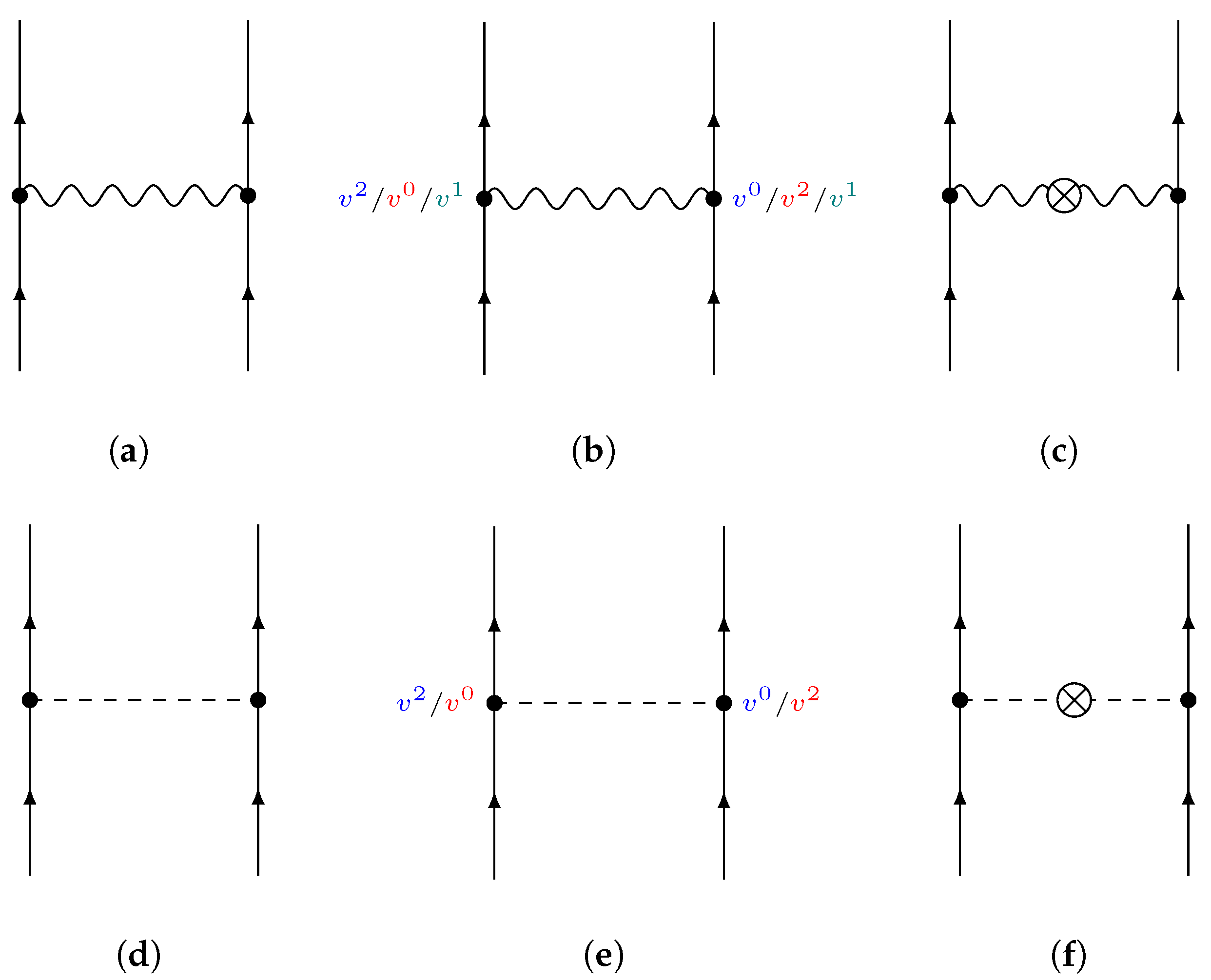
3.1. Velocity Corrections to the 0PN Diagrams

In order to obtain the point-particle action contribution at the next-to-leading order in ${(v/c)}^{2n}$, the so-called 1PN order, both velocity modifications to the previous potentials, as well as higher order terms of the potential, must be accounted for. Diagrammatically, the velocity corrections to the leading order term can be expressed using the Feynman diagrams of Figure 1. Figure 1a,d represent the 0PN contributions already calculated

$$\begin{array}{cc}\hfill V_{\mathrm{Figure\; 1a}}& =-{\displaystyle \frac{G{m}_1{m}_2}{r}},\hfill \end{array}$$

(26a)

$$\begin{array}{cc}\hfill V_{\mathrm{Figure\; 1d}}& =-{\displaystyle \frac{q_1{q}_2}{4\pi r}}.\hfill \end{array}$$

(26b)

Figure 1c,f belongs to the 1PN and represent corrections to the Green’s function, as described in Equation (23):

$$\begin{array}{cc}\hfill V_{\mathrm{Figure\; 1c}}& =-{\displaystyle \frac{G{m}_1{m}_2}{r}}\left({\displaystyle \frac{{\mathit{v}}_1\mathit{·}{\mathit{v}}_2-\left({\mathit{v}}_1\mathit{·}\widehat{\mathit{r}}\right)\left({\mathit{v}}_2\mathit{·}\widehat{\mathit{r}}\right)}{2c^2}}\right),\hfill \end{array}$$

(27a)

$$\begin{array}{cc}\hfill V_{\mathrm{Figure\; 1f}}& =-{\displaystyle \frac{q_1{q}_2}{4\pi r}}\left({\displaystyle \frac{{\mathit{v}}_1\mathit{·}{\mathit{v}}_2-\left({\mathit{v}}_1\mathit{·}\widehat{\mathit{r}}\right)\left({\mathit{v}}_2\mathit{·}\widehat{\mathit{r}}\right)}{2c^2}}\right).\hfill \end{array}$$

(27b)

The last two diagrams, Figure 1b,e, represent general velocity expansion of the interaction term, mainly the expansion of Lorentz factors ${\gamma }_a^{-1}=1-{\displaystyle \frac{v_a^2}{2c^2}}-{\displaystyle \frac{v_a^4}{8c^4}}-\dots$, but for the graviton interaction, one must also include spatial contributions of the source four-velocities, like $h_{ij}{\dot{x}}^i{\dot{x}}^j$ and $h_{0i}{\dot{x}}^0{\dot{x}}^i$.

$$\begin{array}{cc}\hfill V_{\mathrm{Figure\; 1b}}& =\left\{\begin{array}{c}-{\displaystyle \frac{G{m}_1{m}_2}{r}}{\displaystyle \frac{3{\mathit{v}}_1^2}{2c^2}}\hfill \\ -{\displaystyle \frac{G{m}_1{m}_2}{r}}{\displaystyle \frac{3{\mathit{v}}_2^2}{2c^2}}\hfill \\ \phantom{-}{\displaystyle \frac{G{m}_1{m}_2}{r}}{\displaystyle \frac{4{\mathit{v}}_1\mathit{·}{\mathit{v}}_2}{c^2}}\hfill \end{array}\right.,\hfill \end{array}$$

(28a)

$$\begin{array}{cc}\hfill V_{\mathrm{Figure\; 1e}}& =\left\{\begin{array}{c}\phantom{-}{\displaystyle \frac{q_1{q}_2}{4\pi r}}{\displaystyle \frac{{\mathit{v}}_1^2}{2c^2}}\hfill \\ \phantom{-}{\displaystyle \frac{q_1{q}_2}{4\pi r}}{\displaystyle \frac{{\mathit{v}}_2^2}{2c^2}}\hfill \end{array}\right..\hfill \end{array}$$

(28b)

For higher PN orders, these expansions are continued and mixed; for example, they may include a mix of Figure 1b,c, a diagram with two ⊗, and interaction points of the type $v^2-v^2$ and $v^4-v^0$ in analogy to Figure 1b,e. But for the 1PN, Figure 1 contains all the contributing single propagator diagrams.

3.2. Higher-Order Diagrams: Seagull

We here move on to higher-order diagrams, that is, diagrams of higher-order powers of the fields $h_{\mu \nu }$ and K. Figure 3 depicts the next-to-leading order interaction terms of Equation (16), namely Figure 3a $\simeq m_a{c}^2\times {\displaystyle \frac{1}{8}}{\left(\lambda h_{\mu \nu }{\displaystyle \frac{{\dot{x}}^{\mu }}{c}}{\displaystyle \frac{{\dot{x}}^{\nu }}{c}}\right)}^2$, Figure 3b $\simeq p_a{K}^2\times \left(-1\right)$, and Figure 3c $\simeq q_{a}K\times {\displaystyle \frac{1}{2}}\lambda h_{\mu \nu }{\displaystyle \frac{{\dot{x}}^{\mu }}{c}}{\displaystyle \frac{{\dot{x}}^{\nu }}{c}}$. Inserting the leading order solution for $\lambda h_{00}\left(x\right)={\sum }_b{\displaystyle \frac{{\lambda }^2{m}_b{\gamma }_b{c}^2\delta (x^0-x_b^0)}{8\pi |\mathit{x}-{\mathit{x}}_b|}}$ and $K\left(x\right)={\sum }_b-{\displaystyle \frac{{\gamma }_b^{-1}{q}_b\delta (x^0-x_b^0)}{4\pi |\mathit{x}-{\mathit{x}}_b|}}$, the resulting terms of the action originating from these diagrams and subsequently their potential are easily obtained.

$$\begin{array}{cc}\hfill V_{\mathrm{Figure\; 3a}}& =-{\displaystyle \frac{G^2(m_1{m}_2^2+m_2{m}_1^2)}{2c^2{r}^2}},\hfill \end{array}$$

(29a)

$$\begin{array}{cc}\hfill V_{\mathrm{Figure\; 3b}}& =\phantom{-}{\displaystyle \frac{(p_1{q}_2^2+p_2{q}_1^2)}{16{\pi }^2{r}^2}},\hfill \end{array}$$

(29b)

$$\begin{array}{cc}\hfill V_{\mathrm{Figure\; 3c}}& =\phantom{-}{\displaystyle \frac{G{q}_1{q}_2(m_1+m_2)}{4\pi c^2{r}^2}}.\hfill \end{array}$$

(29c)

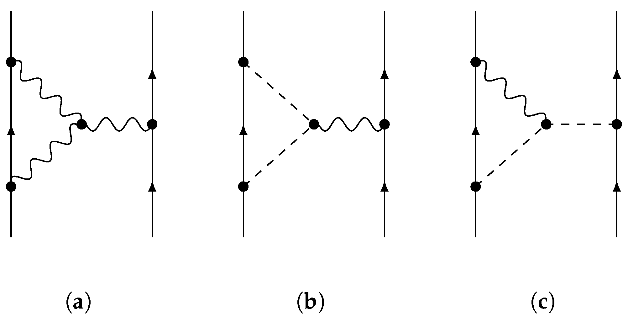
3.3. Higher-Order Diagrams: Field Interactions

The last set of diagrams contributing to the 1PN action originates from corrections to the solution of the fields themselves; see Equations (19) and (20). They are depicted diagrammatically in Figure 4 as field-interactions. The explicit form of the action term is here

$$\begin{array}{c}\hfill S_{\mathrm{Figure\; 4}}=\int {\displaystyle \frac{{\mathrm{d}}^{4}x}{c}}\sum _a{\gamma }_a^{-1}\left[{\displaystyle \frac{m_a\lambda }{2}}{h}_{00}^{\left(2\right)}\left(x\right){\left({\gamma }_{a}c\right)}^2-q_a{K}^{\left(2\right)}\left(x\right)\right]{\delta }^3\left(\mathit{x}-{\mathit{x}}_a\left(x^0\right)\right),\end{array}$$

(30)

where the corrections in the fields $h_{00}^{\left(2\right)}\left(x\right)$ and $K^{\left(2\right)}\left(x\right)$ are the items of interest.

3.3.1. The Corresponding Potential of Figure 4a

Figure 4a originates from the graviton energy-momentum (pseudo-)tensor $t^{\alpha \beta }$ contribution to the equation of motion (17) with the corresponding solution:

$$\begin{array}{c}\hfill \begin{array}{c}\hfill h_{00}^{\left(2\right)}\left(x\right)\ni -\lambda \int {\mathrm{d}}^{4}y\Delta (x^{\sigma }-y^{\sigma })P_{00\alpha \beta }{\displaystyle \frac{1}{2}}{h_{\mu \nu }}^{,\alpha }{h}^{\mu \nu ,\beta }.\end{array}\end{array}$$

(31)

To solve this, one can write out the $h_{\mu \nu }$ fields as their leading-order solution in Fourier space, as follows:

$$\begin{array}{cc}\hfill {h_{\mu \nu }}^{,\alpha }\left(y\right)=& -\lambda \int \int {\displaystyle \frac{{\mathrm{d}}^{4}p}{{\left(2\pi \right)}^4}}{\displaystyle \frac{i{p}^{\alpha }{e}^{i{k}_{\rho }\left(y^{\rho }-z^{\rho }\right)}}{-p_{\sigma }{p}^{\sigma }}}{p}_{\mu \nu 00}{T}^{00}\left(z\right){\mathrm{d}}^{4}z,\hfill \end{array}$$

(32)

$$\begin{array}{cc}\hfill & P_{\mu \nu 00}=P_{00\mu \nu }={\displaystyle \frac{1}{2}}{\delta }_{\mu \nu }.\hfill \end{array}$$

(33)

For algebraic convenience, one might also utilise the following relation valid for any field $\Phi$ and $\Theta$:

$$\begin{array}{c}\hfill {\Phi }_{,\{\alpha }{\Theta }_{,\beta \}}={\displaystyle \frac{1}{2}}\left({\left(\Phi \Theta \right)}_{,\alpha \beta }-{\Phi }_{,\alpha \beta }\Theta -\Phi {\Theta }_{,\alpha \beta }\right).\end{array}$$

(34)

Using the notation $\int {\displaystyle \frac{{\mathrm{d}}^{4}k}{{\left(2\pi \right)}^4}}={\int }_k$, and taking advantage of rewriting the derivatives in accordance with (34), one obtains

$$\begin{array}{c}\hfill \begin{array}{c}\hfill h_{00}^{\left(2\right)}\left(x\right)\ni -{\lambda }^3\int {\int }_k{\int }_{p_1,p_2}{\displaystyle \frac{e^{i{k}_{\sigma }(x^{\sigma }-y^{\sigma })}}{k_{\sigma }{k}^{\sigma }}}{\displaystyle \frac{e^{i{p}_{1\sigma }(y^{\sigma }-z_1^{\sigma })}}{p_{1\sigma }{p}_1^{\sigma }}}{\displaystyle \frac{e^{i{p}_{2\sigma }(y^{\sigma }-z_2^{\sigma })}}{p_{2\sigma }{p}_2^{\sigma }}}{\displaystyle \frac{1}{8}}{\delta }_{\alpha \beta }·\\ \hfill \left[(p_1^{\alpha }+p_2^{\alpha })(p_1^{\beta }+p_2^{\beta })-p_1^{\alpha }{p}_1^{\beta }-p_2^{\alpha }{p}_2^{\beta }\right]T^{00}\left(z_1\right)T^{00}\left(z_1\right){\mathrm{d}}^{4}y\end{array}\end{array}$$

(35)

Separating out all the factors of y and integrating over y results in a conservation-of-momentum factor

$$\begin{array}{c}\hfill \int e^{-i{y}^{\mu }\left(k_{\mu }-p_{1\mu }-p_{2\mu }\right)}{\mathrm{d}}^{4}y={\left(2\pi \right)}^4{\delta }^4\left(k_{\mu }-p_{1\mu }-p_{2\mu }\right).\end{array}$$

Then, performing the k integral sets $k_{\mu }=p_{1\mu }+p_{2\mu }\equiv q_{\mu }$, and tidying up the expression gives

$$\begin{array}{cc}\hfill h_{00}^{\left(2\right)}\left(x\right)\ni -{\lambda }^3{\int }_{p_1,p_2}{\displaystyle \frac{e^{i{q}_{\sigma }{x}^{\sigma }}}{q_{\sigma }{q}^{\sigma }}}{\displaystyle \frac{e^{-i{p}_{1\sigma }{z}_1^{\sigma }}}{p_{1\sigma }{p}_1^{\sigma }}}{\displaystyle \frac{e^{-i{p}_{2\sigma }{z}_2^{\sigma }}}{p_{2\sigma }{p}_2^{\sigma }}}{\displaystyle \frac{1}{8}}{\delta }_{\alpha \beta }& \left[q^{\alpha }{q}^{\beta }-p_1^{\alpha }{p}_1^{\beta }-p_2^{\alpha }{p}_2^{\beta }\right]T^{00}\left(z_1\right)T^{00}\left(z_2\right).\hfill \end{array}$$

(36)

The final step is to again let ${\displaystyle \frac{1}{k_{\mu }{k}^{\mu }}}\to {\displaystyle \frac{1}{k^2}}$ and likewise ignore factors of $p^0$ appearing in the numerator, as these also will result in velocity corrections and thus belong in higher-PN-order terms; see Equation (23). Then we finally have

$$\begin{array}{cc}\hfill h_{00}^{\left(2\right)}\left(x\right)\ni -{\displaystyle \frac{{\lambda }^3}{8}}{\int }_{p_1,p_2}& {\displaystyle \frac{e^{i{q}_{\sigma }{x}^{\sigma }}}{{\mathit{q}}^2}}{\displaystyle \frac{e^{-i{p}_{1\sigma }{z}_1^{\sigma }}}{{\mathit{p}}_1^2}}{\displaystyle \frac{e^{-i{p}_{2\sigma }{z}_2^{\sigma }}}{{\mathit{p}}_2^2}}\left[{\mathit{q}}^2-{\mathit{p}}_1^2-{\mathit{p}}_2^2\right]T^{00}\left(z_1\right)T^{00}\left(z_2\right)\hfill \\ \hfill =-{\displaystyle \frac{{\lambda }^3}{8}}{\int }_{p_1,p_2}& [{\displaystyle \frac{e^{i{p}_{1\sigma }(x^{\sigma }-z_1^{\sigma })}}{{\mathit{p}}_1^2}}{\displaystyle \frac{e^{i{p}_{2\sigma }(x^{\sigma }-z_2^{\sigma })}}{{\mathit{p}}_2^2}}-{\displaystyle \frac{e^{i{q}_{\sigma }(x^{\sigma }-z_1^{\sigma })}}{{\mathit{q}}^2}}{\displaystyle \frac{e^{i{p}_{2\sigma }(z_1^{\sigma }-z_2^{\sigma })}}{{\mathit{p}}_2^2}}\hfill \\ \hfill & -{\displaystyle \frac{e^{i{q}_{\sigma }(x^{\sigma }-z_2^{\sigma })}}{{\mathit{q}}^2}}{\displaystyle \frac{e^{i{p}_{2\sigma }(z_2^{\sigma }-z_1^{\sigma })}}{{\mathit{p}}_1^2}}]T^{00}\left(z_1\right)T^{00}\left(z_2\right).\hfill \end{array}$$

(37)

In the first term ${\mathit{q}}^2$, the first denominator is cancelled, and remembering that $q^{\mu }=p_1^{\mu }+p_2^{\mu }$, the remaining exponential factor can be split up and distributed into the remaining exponential factors. Thus, the first term is as follows:

$$\begin{array}{c}\hfill \begin{array}{cc}\hfill & -{\displaystyle \frac{{\lambda }^3}{8}}{\int }_{p_1,p_2}{\displaystyle \frac{e^{i{p}_{1\sigma }\left(x^{\sigma }-z_1^{\sigma }\right)}}{{\mathit{p}}_1^2}}{\displaystyle \frac{e^{i{p}_{2\sigma }\left(x^{\sigma }-z_2^{\sigma }\right)}}{{\mathit{p}}_2^2}}{T}^{00}\left(z_1\right)T^{00}\left(z_2\right)\hfill \\ \hfill & =-{\displaystyle \frac{{\lambda }^3}{8}}{\Delta }_{\mathrm{inst}}^{\left(0\right)}(x^{\mu }-z_1^{\mu }){\Delta }_{\mathrm{inst}}^{\left(0\right)}(x^{\mu }-z_2^{\mu })T^{00}\left(z_1\right)T^{00}\left(z_2\right).\hfill \end{array}\end{array}$$

(38)

The procedure is the same for the two last terms of (37), with the addition of shifting one of the integration variables to $q^{\mu }$.

Returning to the action (30) for Figure 4a, we have

$$\begin{array}{cc}\hfill S_{\mathrm{Figure\; 4a}}=& \int \sum _{a\ne b,c}{\displaystyle \frac{{\lambda }^4{m}_a{m}_b{m}_c{c}^6}{16{\left(4\pi \right)}^2}}({\displaystyle \frac{-1}{|{\mathit{x}}_a-{\mathit{z}}_b|·|{\mathit{x}}_a-{\mathit{z}}_c|}}\hfill \\ \hfill & +{\displaystyle \frac{1}{|{\mathit{x}}_a-{\mathit{z}}_b|·|{\mathit{z}}_b-{\mathit{z}}_c|}}+{\displaystyle \frac{1}{|{\mathit{x}}_a-{\mathit{z}}_c|·|{\mathit{z}}_c-{\mathit{z}}_b|}})\mathrm{d}t\hfill \end{array}$$

$$\begin{array}{cc}\hfill =& \int -{\displaystyle \frac{G^2{m}_1{m}_2(m_1+m_2)}{c^2{r}^2}}\mathrm{d}t,\hfill \end{array}$$

(39)

$$\begin{array}{cc}\hfill V_{\mathrm{Figure\; 4a}}=& {\displaystyle \frac{G^2{m}_1{m}_2(m_1+m_2)}{c^2{r}^2}}.\hfill \end{array}$$

(40)

The purpose of the requirement $b\ne a\ne c$ of the sum is to make sure the gravitational potential acting on particle number a is not sourced by itself. Discarding then all divergent terms8$\propto {\displaystyle \frac{1}{|z_i-z_i|}}$, one is left with the potential (40).

3.3.2. The Corresponding Potential of Figure 4b

Figure 4b is quite similar to Figure 4a but accounts for the Kalb–Ramond scalar contribution to $h_{00}^{\left(2\right)}\left(x\right)$ from the equation of motion (17):

$$\begin{array}{cc}\hfill h_{00}^{\left(2\right)}\left(x\right)\ni & \lambda \int {\mathrm{d}}^{4}y\Delta (x^{\sigma }-y^{\sigma })P_{00\alpha \beta }\left\{{\displaystyle \frac{1}{2}}{\eta }^{\alpha \beta }{K}_{,\sigma }\left(y\right)K^{,\sigma }\left(y\right)+K^{,\alpha }\left(y\right)K^{,\beta }\left(y\right)\right\}\hfill \end{array}$$

(41a)

$$\begin{array}{c}\hfill \begin{array}{cc}\hfill & ={\displaystyle \frac{i^2\lambda }{2}}{\int }_{p_1,p_2}{\displaystyle \frac{e^{i{q}_{\mu }{x}^{\mu }}}{-{\mathit{q}}^2}}{\displaystyle \frac{e^{-i{p}_{1\mu }{z}_1^{\mu }}}{-{\mathit{p}}_1^2}}{\displaystyle \frac{e^{-i{p}_{2\mu }{z}_2^{\mu }}}{-{\mathit{p}}_2^2}}\left[{\mathit{q}}^2-{\mathit{p}}_1^2-{\mathit{p}}_2^2\right]J\left(z_1\right)J\left(z_2\right),\hfill \end{array}\end{array}$$

(41b)

where, again, $q^{\mu }=p_1^{\mu }+p_2^{\mu }$. These integrals are identical to the ones found in (37) and are solved the same way.

$$\begin{array}{c}\hfill \begin{array}{cc}\hfill h_{00}^{\left(2\right)}\ni & {\displaystyle \frac{\lambda }{2}}[{\Delta }_{\mathrm{inst}}(x-z_1){\Delta }_{\mathrm{inst}}(x-z_2)-{\Delta }_{\mathrm{inst}}(x-z_1){\Delta }_{\mathrm{inst}}(z_1-z_2)\hfill \\ \hfill & -{\Delta }_{\mathrm{inst}}(x-z_2){\Delta }_{\mathrm{inst}}(z_2-z_1)]J\left(z_1\right)J\left(z_2\right)\hfill \\ \hfill =& \sum _{b,c}{\displaystyle \frac{\lambda q_b{q}_c}{32{\pi }^2}}\left[{\displaystyle \frac{1}{|\mathit{x}-{\mathit{z}}_b|·|\mathit{x}-{\mathit{z}}_c|}}-{\displaystyle \frac{1}{|\mathit{x}-{\mathit{z}}_b|·|{\mathit{z}}_b-{\mathit{z}}_c|}}-{\displaystyle \frac{1}{|\mathit{x}-{\mathit{z}}_c|·|{\mathit{z}}_c-{\mathit{z}}_b|}}\right].\hfill \end{array}\end{array}$$

(42)

On substituting this result back into the action (30), we can derive the associated potential.

$$\begin{array}{cc}\hfill S_{\mathrm{Figure\; 4b}}& =\int \sum _{a\ne b,c}{\displaystyle \frac{{\lambda }^2{m}_a{q}_b{q}_c{c}^2}{64{\pi }^2}}({\displaystyle \frac{1}{|\mathit{x}-{\mathit{z}}_b|·|\mathit{x}-{\mathit{z}}_c|}}\hfill \\ \hfill & -{\displaystyle \frac{1}{|\mathit{x}-{\mathit{z}}_b|·|{\mathit{z}}_b-{\mathit{z}}_c|}}-{\displaystyle \frac{1}{|\mathit{x}-{\mathit{z}}_c|·|{\mathit{z}}_c-{\mathit{z}}_b|}})\mathrm{d}t\hfill \end{array}$$

$$\begin{array}{cc}\hfill & =\int {\displaystyle \frac{G(m_1{q}_2^2+m_2{q}_1^2)}{4\pi r^2{c}^2}}\mathrm{d}t,\hfill \end{array}$$

(43)

$$\begin{array}{cc}\hfill V_{\mathrm{Figure\; 4b}}& =-{\displaystyle \frac{G(m_1{q}_2^2+m_2{q}_1^2)}{4\pi r^2{c}^2}}.\hfill \end{array}$$

(44)

3.3.3. The Corresponding Potential of Figure 4c

For Figure 4c, the next-to-leading-order terms in the equation of motion for the Kalb–Ramond scalar (18) are included.

$$\begin{array}{c}\hfill K^{\left(2\right)}\left(x\right)=-\lambda \int {\mathrm{d}}^{4}y\Delta (x^{\sigma }-y^{\sigma })\left(h^{\mu \nu }{K}_{,\mu \nu }+{h^{\mu \nu }}_{,\mu }{K}_{,\nu }+{\displaystyle \frac{1}{2}}\left(h_{,\mu }{K}^{,\mu }+h\square K\right)\right).\end{array}$$

(45)

Since the derivative indices are contracted either with themselves or with the graviton field $h^{\mu \nu }{\partial }_{\mu }{\partial }_{\nu }$, they are symmetric under $\mu \leftrightarrow \nu$, and one may therefore also use (34) in this context. Using this and the other tricks shown in Figure 4a,b, one can demonstrate

$$\begin{array}{c}\hfill \begin{array}{cc}\hfill K^{\left(2\right)}\left(x\right)=& -{\displaystyle \frac{i^2{\lambda }^2}{2}}{\int }_{p,k}{\displaystyle \frac{e^{i{q}_{\sigma }{x}^{\sigma }}}{-{\mathit{q}}^2}}{\displaystyle \frac{e^{-i{k}_{\sigma }{z}_b^{\sigma }}}{{\mathit{k}}^2}}{\displaystyle \frac{e^{-i{p}_{\sigma }{z}_c^{\sigma }}}{-{\mathit{p}}^2}}\left({\mathit{q}}^2+{\mathit{p}}^2-{\mathit{k}}^2\right)T_{00}\left(z_b\right)J\left(z_c\right)\hfill \\ \hfill =& \sum _{b,c}{\displaystyle \frac{{\lambda }^2{m}_b{q}_c{c}^2}{32{\pi }^2}}({\displaystyle \frac{1}{|\mathit{x}-{\mathit{z}}_b|·|\mathit{x}-{\mathit{z}}_c|}}+{\displaystyle \frac{1}{|\mathit{x}-{\mathit{z}}_c|·|{\mathit{z}}_c-{\mathit{z}}_b|}}\hfill \\ \hfill & -{\displaystyle \frac{1}{|\mathit{x}-{\mathit{z}}_b|·|{\mathit{z}}_b-{\mathit{z}}_c|}}).\hfill \end{array}\end{array}$$

(46)

Again, $q^{\mu }=k^{\mu }+p^{\mu }$.

$$\begin{array}{cc}\hfill S_{\mathrm{Figure\; 4c}}=\int \sum _{a\ne b,c}{\displaystyle \frac{G{q}_a{m}_b{q}_c}{2\pi c^2}}& \left({\displaystyle \frac{1}{|\mathit{x}-{\mathit{z}}_b|·|\mathit{x}-{\mathit{z}}_c|}}+{\displaystyle \frac{1}{|\mathit{x}-{\mathit{z}}_c|·|{\mathit{z}}_c-{\mathit{z}}_b|}}-{\displaystyle \frac{1}{|\mathit{x}-{\mathit{z}}_b|·|{\mathit{z}}_b-{\mathit{z}}_c|}}\right)\mathrm{d}t\hfill \\ \hfill & V_{\mathrm{Figure\; 4c}}=-{\displaystyle \frac{G{q}_1{q}_2(m_1+m_2)}{2\pi r^2{c}^2}}\hfill \end{array}$$

(47)

Notice how $V_{\mathrm{Figure\; 4c}}=-2·V_{\mathrm{Figure\; 3c}}$ and will thus ‘destructively interfere’ with one another, analogous to how $V_{\mathrm{Figure\; 4a}}=-2·V_{\mathrm{Figure\; 3a}}$ in GR.

4. The Resulting Binary Lagrangian

The kinetic term of the binary Lagrangian is obtained from Equation (16) from the cross-term ${\sum }_a{\gamma }_a^{-1}{m}_a{c}^2\times (-1)$ and by expanding the Lorentz factor in powers of velocity. To 1PN, this is

$$\begin{array}{c}\hfill \begin{array}{cc}\hfill L_{pp}^{\mathrm{kin}}& =\sum _a-m_a{c}^2+{\displaystyle \frac{1}{2}}{m}_a{v}_a^2+{\displaystyle \frac{1}{8}}{m}_a{\displaystyle \frac{v_a^4}{c^2}}+\mathcal{O}\left({\displaystyle \frac{v^6}{c^4}}\right)\hfill \\ \hfill & =-M{c}^2+{\displaystyle \frac{1}{2}}\mu v^2+{\displaystyle \frac{1-3\eta }{8}}\mu {\displaystyle \frac{v^4}{c^2}}+\mathcal{O}\left({\displaystyle \frac{v^6}{c^4}}\right).\hfill \end{array}\end{array}$$

(48)

The constant term can be ignored for all dynamical purposes. In the last line, effective one-body coordinates have been implemented, where M is the total mass $M=m_1+m_2$, $\mu$ is the reduced mass $\mu ={\displaystyle \frac{m_1{m}_2}{m_1+m_2}}$, $\eta$ is the symmetric mass ratio $\eta ={\displaystyle \frac{\mu }{M}}={\displaystyle \frac{m_1{m}_2}{{(m_1+m_2)}^2}}$, and v is the relative velocity $\mathit{v}=\dot{\mathit{r}}={\mathit{v}}_1-{\mathit{v}}_2$ when $\mathit{r}={\mathit{r}}_1-{\mathit{r}}_2$.

The contributions from standard general relativity are derived from all the diagrams containing only graviton propagators

$$\begin{array}{cc}\hfill L_{pp}^{\mathrm{GR}}=& {\displaystyle \frac{G{m}_1{m}_2}{r}}\left(1+{\displaystyle \frac{3}{2}}{\displaystyle \frac{v_1^2+v_2^2}{c^2}}-{\displaystyle \frac{4{\mathit{v}}_1\mathit{·}{\mathit{v}}_2}{c^2}}+{\displaystyle \frac{{\mathit{v}}_1\mathit{·}{\mathit{v}}_2-({\mathit{v}}_1\mathit{·}\widehat{\mathit{r}})({\mathit{v}}_2\mathit{·}\widehat{\mathit{r}})}{2c^2}}-{\displaystyle \frac{G(m_1+m_2)}{2r{c}^2}}\right)\hfill \\ \hfill =& {\displaystyle \frac{GM\mu }{r}}\left(1+3{\displaystyle \frac{1-2\eta }{2}}{\displaystyle \frac{v^2}{c^2}}+{\displaystyle \frac{4\eta v^2}{c^2}}-\eta {\displaystyle \frac{v^2-{\left(\mathit{v}\mathit{·}\widehat{\mathit{r}}\right)}^2}{2c^2}}-{\displaystyle \frac{GM}{2r{c}^2}}\right)+\mathcal{O}\left({\displaystyle \frac{v^3}{c^3}}\right).\hfill \end{array}$$

(49)

Next, the additional potentials from the inclusion of the Kalb–Ramond (effectively scalar) field:

$$\begin{array}{cc}\hfill L_{pp}^{\mathrm{KR}}=& {\displaystyle \frac{q_1{q}_2}{4\pi r}}(1-{\displaystyle \frac{v_1^2+v_2^2}{2c^2}}+{\displaystyle \frac{{\mathit{v}}_1\mathit{·}{\mathit{v}}_2-({\mathit{v}}_1\mathit{·}\widehat{\mathit{r}})({\mathit{v}}_2\mathit{·}\widehat{\mathit{r}})}{2c^2}}\hfill \\ \hfill & \left.-{\displaystyle \frac{\left(\frac{p_1{q}_2}{q_1}+\frac{p_2{q}_1}{q_2}\right)}{4\pi r}}+{\displaystyle \frac{G(m_1+m_2)}{r{c}^2}}+{\displaystyle \frac{G\left(\frac{m_1{q}_2}{q_1}+\frac{m_2{q}_1}{q_2}\right)}{r{c}^2}}\right)\hfill \\ \hfill =& {\displaystyle \frac{q_1{q}_2}{4\pi r}}\left(1-{\displaystyle \frac{1-2\eta }{2}}{\displaystyle \frac{v^2}{c^2}}-\eta {\displaystyle \frac{v^2-{\left(\mathit{v}\mathit{·}\widehat{\mathit{r}}\right)}^2}{2c^2}}-{\displaystyle \frac{p}{4\pi r}}+{\displaystyle \frac{GM}{r{c}^2}}+{\displaystyle \frac{G\left(\frac{m_1{q}_2}{q_1}+\frac{m_2{q}_1}{q_2}\right)}{r{c}^2}}\right).\hfill \end{array}$$

(50)

In the last line, $p={\displaystyle \frac{p_1{q}_2}{q_1}}+{\displaystyle \frac{p_2{q}_1}{q_2}}$. Notice that if $p_a\propto q_a$, it follows that $p\propto q_1+q_2$, i.e., the total charge, making it analogous to how Figure 3a is a factor of total mass correction to Newton’s potential in GR ($V_{\mathrm{Figure\; 3a}}=-{\displaystyle \frac{GM\mu }{r}}·{\displaystyle \frac{-GM}{2r{c}^2}}$).

For comparison, here is the Lagrangian obtained by Huang et al. for axions in [10], rewritten to have notation consistent with that used in this paper:

$$\begin{array}{cc}\hfill L_{pp}^{\varphi }=& {\displaystyle \frac{q_1{q}_2}{4\pi r}}{e}^{-m_{s}r}\left(1+{\displaystyle \frac{{\mathit{v}}_1\mathit{·}{\mathit{v}}_2-({\mathit{v}}_1\mathit{·}\widehat{\mathit{r}})({\mathit{v}}_2\mathit{·}\widehat{\mathit{r}})(1+m_{s}r)}{2c^2}}-{\displaystyle \frac{p·e^{-m_{s}r}}{2\pi r}}-{\displaystyle \frac{GM}{r{c}^2}}\right)\hfill \\ \hfill & -{\displaystyle \frac{G(m_1{q}_2^2+m_2{q}_1^2)}{16\pi r^2}}{m}_{s}r\left[e^{-2m_{s}r}+2m_{s}r\mathrm{Ei}(-2m_{s}r)\right]+{\displaystyle \frac{GM{q}_1{q}_2}{2\pi r^2{c}^2}}{m}_{s}r\mathcal{I}\left(m_{s}r\right).\hfill \end{array}$$

(51)

Here, $\mathcal{I}\left(x\right)\equiv {\displaystyle \frac{2}{\pi }}{\int }_0^{\infty }{\displaystyle \frac{\mathrm{d}k}{k^2+1}}sin\left(kx\right)arctan\left(k\right)$ and $\mathrm{Ei}\left(x\right)\equiv -{\int }_{-x}^{\infty }{\displaystyle \frac{e^{-t}}{t}}\mathrm{d}t$. In the massless $m_s\to 0$ limit of Equation (51), many but not all terms are the same as in Equation (50). In particular, the terms with an explicit factor of $m_s$ vanish in this limit, originating from diagrams like Figure 4b,c. Additionally, the terms proportional to the squared velocity are missing from the Lagrangian in [10].

Some Observable Consequences

Equipped with the Lagrangian up to the first post-Newtonian order for a binary system under the influence of gravity, obtained by combining Equations (48) and (49) and adding the Kalb–Ramond Lagrangian (50), it is straightforward to compute observable effects on binary systems, as described in the book [34]. Chiefly, the resulting equation of motion for the system is computed to be

$$\begin{array}{cc}\hfill & {\omega }^4+\left({\displaystyle \frac{\mu r+\frac{GM\mu }{c^2}\left(\frac{3}{2}+\frac{\eta }{2}\right)+\frac{q_1{q}_2}{4\pi c^2}\left(-\frac{1}{2}+\frac{\eta }{2}\right)}{\mu r^3\frac{1-3\eta }{2c^2}}}\right){\omega }^2\hfill \\ \hfill & -{\displaystyle \frac{\left(GM\mu +\frac{q_1{q}_2}{4\pi }\right)r-\frac{G^2{M}^2\mu }{c^2}-\frac{q_1{q}_{2}p}{8{\pi }^2}+\frac{G(M{q}_1{q}_2+m_1{q}_2^2+m_2{q}_1^2)}{2\pi c^2}}{\frac{1-3\eta }{2c^2}\mu r^6}}=0.\hfill \end{array}$$

(52)

Here, quasi-circular motion has been assumed, neglecting terms proportional to $\dot{r}$ and $\ddot{r}$. Then, Equation (52) can be used to find the relationship between the orbital frequency $\omega$ and separation r up to the 1PN order:

$$\begin{array}{cc}\hfill r\left(\omega \right)=& {\displaystyle \frac{4\pi GM\mu +q_1{q}_2}{4\pi \mu }}{\left({\displaystyle \frac{(4\pi GM\mu +q_1{q}_2)\omega }{4\pi \mu }}\right)}^{-2/3}\{1+\hfill \\ \hfill & (-{\displaystyle \frac{G^2{M}^2{\mu }^3}{2c^2}}-{\displaystyle \frac{{\mu }^2{q}_1{q}_{2}p}{16{\pi }^2}}+{\displaystyle \frac{G(M{\mu }^2{q}_1{q}_2+{\mu }^2{m}_1{q}_2^2+{\mu }^2{m}_2{q}_1^2)}{4\pi c^2}}\hfill \\ \hfill & -{\displaystyle \frac{2GM{\mu }^2+\frac{q_1{q}_2\mu }{2\pi }}{4c^2}}\left(GM\mu (3+\eta )+{\displaystyle \frac{q_1{q}_2(-1+\eta )}{4\pi }}\right)\hfill \\ \hfill & -{\displaystyle \frac{(1-3\eta )\mu {\left(4\pi GM\mu +q_1{q}_2\right)}^2}{64{\pi }^2{c}^2}})/\left({\displaystyle \frac{3}{2}}\mu {\left({\displaystyle \frac{4\pi GM\mu +q_1{q}_2}{4\pi }}\right)}^2\right)\hfill \\ \hfill & ·{\left({\displaystyle \frac{(4\pi GM\mu +q_1{q}_2)\omega }{4\pi \mu }}\right)}^{2/3}+\dots \}.\hfill \end{array}$$

(53)

Adopting the limit found in [10] for $|q_i|=5.7·{10}^{-7}\sqrt{G}{m}_i$ and $p={\displaystyle \frac{R_1^{\mathrm{NS}}+R_2^{\mathrm{NS}}}{16G}}$ for binary neutron stars of roughly equal mass, we find using (52) the spacial separation correction for a system with $m_1=1.20M_{\odot }$ and $m_2=1.24M_{\odot }$, orbiting at $\omega =50\mathrm{Hz}$9 to be $\delta r=r_{1\mathrm{PN}}-r_{0\mathrm{PN}}=3.3\mathrm{km}$. This is a correction of $0.6\%$ to $r\left(\omega \right)$ with $q_i=0$ and $p_i=0$. In order for that correction to be ≥1%, the charge would have to scale as $|q_i|\ge 11\sqrt{G}{m}_i$.

Another result is obtained by applying this to the Earth–Moon system. Still assuming circular orbits and the charge scaling found in [10], one finds $\delta r\approx 4\mathrm{mm}$, but this is the same result found in pure GR, making the difference from including the Kalb–Ramond field negligible.

Further consequences to the orbital dynamics can be calculated using the Lagrangian and the wealth of formulas and resources found in [34].

5. Conclusions and Outlook

We have derived the leading-order relativistic Lagrangian corrections for a Kalb–Ramond field coupled to gravity: Equation (50). Our computation would apply in the relativistic regime, but not the quantum regime. Astrophysical compact objects may or may not have measurable Kalb–Ramond charge. In the stringy fuzzball proposal, black holes are composed of macroscopic strings [16], and these may well have non-zero Kalb–Ramond charge. Fuzzballs should potentially also have non-trivial dilation profiles, as is seen in other black-hole solutions in dilaton gravity and supergravity [12,13,35]. Unlike the Kalb–Ramond (and photon) field, the dilaton is not protected by a symmetry and so can dynamically acquire a mass, making the force short-range even at the classical level. If macroscopic strings exist at cosmological scales, then they may also interact via a Kalb–Ramond-mediated force [15].

In our derived Lagrangian, note the similar $\frac{1}{r}$-behaviours in the relativistic expansions for both the Kalb–Ramond and classical General Relativity corrections. This is perhaps not too surprising in view of generalised geometry, where the metric and Kalb–Ramond fields are put on the same footing in the generalised metric [27,28,29]. This point of view also leads us to speculate that this similar behaviour will persist to higher orders. In order to investigate this further, it would be very useful to extend the perturbative Feynman diagram formalism of [22,23] to the generalised framework. This framework will also be relevant when we come to understand the theory in higher dimensions or with quantum corrections, where the Kalb–Ramond field can no longer be treated as a scalar.

The approach presented here also demonstrates the power of the effective field theory approach to classifying and calculating possible deviations from Einstein’s theory of gravity. This is relevant in an era of precision pulsar and gravitational wave observations that are testing Einstein’s theory in the strongly relativistic regime.

References

1. Peccei, R.D.; Quinn, H.R. CP Conservation in the Presence of Instantons. Phys. Rev. Lett. 1977, 38, 1440–1443. [Google Scholar] [CrossRef]
2. Wilczek, F. Problem of Strong P and T Invariance in the Presence of Instantons. Phys. Rev. Lett. 1978, 40, 279–282. [Google Scholar] [CrossRef]
3. Weinberg, S. A New Light Boson? Phys. Rev. Lett. 1978, 40, 223–226. [Google Scholar] [CrossRef]
4. Kim, J.E. Weak Interaction Singlet and Strong CP Invariance. Phys. Rev. Lett. 1979, 43, 103. [Google Scholar] [CrossRef]
5. Vafa, C.; Witten, E. Parity Conservation in QCD. Phys. Rev. Lett. 1984, 53, 535. [Google Scholar] [CrossRef]
6. Grilli di Cortona, G.; Hardy, E.; Pardo Vega, J.; Villadoro, G. The QCD axion, precisely. J. High Energy Phys. 2016, 1, 034. [Google Scholar] [CrossRef]
7. Svrcek, P.; Witten, E. Axions in String Theory. J. High Energy Phys. 2006, 6, 051. [Google Scholar] [CrossRef]
8. Arvanitaki, A.; Dimopoulos, S.; Dubovsky, S.; Kaloper, N.; March-Russell, J. String Axiverse. Phys. Rev. D 2010, 81, 123530. [Google Scholar] [CrossRef]
9. Marsh, D.J.E. Axion Cosmology. Phys. Rept. 2016, 643, 1–79. [Google Scholar] [CrossRef]
10. Huang, J.; Johnson, M.C.; Sagunski, L.; Sakellariadou, M.; Zhang, J. Prospects for axion searches with Advanced LIGO through binary mergers. Phys. Rev. D 2019, 99, 063013. [Google Scholar] [CrossRef]
11. Kalb, M.; Ramond, P. Classical direct interstring action. Phys. Rev. D 1974, 9, 2273–2284. [Google Scholar] [CrossRef]
12. Burgess, C.P.; Myers, R.C.; Quevedo, F. On spherically symmetric string solutions in four-dimensions. Nucl. Phys. B 1995, 442, 75–96. [Google Scholar] [CrossRef]
13. Kang, S.; Yeom, D.H. Causal structures and dynamics of black-hole-like solutions in string theory. Eur. Phys. J. C 2019, 79, 927. [Google Scholar] [CrossRef]
14. Afzal, A.; Agazie, G.; Anumarlapudi, A.; Archibald, A.M.; Arzoumanian, Z.; Baker, P.T.; Bécsy, B.; Blanco-Pillado, J.J.; Blecha, L.; Boddy, K.K.; et al. The NANOGrav 15 yr Data Set: Search for Signals from New Physics. Astrophys. J. Lett. 2023, 951, L11. [Google Scholar] [CrossRef]
15. Copeland, E.J.; Myers, R.C.; Polchinski, J. Cosmic F and D strings. J. High Energy Phys. 2004, 6, 013. [Google Scholar] [CrossRef]
16. Mathur, S.D. The Fuzzball proposal for black holes: An Elementary review. Fortsch. Phys. 2005, 53, 793–827. [Google Scholar] [CrossRef]
17. Kramer, M.; Stairs, I.H.; Manchester, R.N.; Wex, N.; Deller, A.T.; Coles, W.A.; Ali, M.; Burgay, M.; Camilo, F.; Cognard, I.; et al. Strong-Field Gravity Tests with the Double Pulsar. Phys. Rev. X 2021, 11, 041050. [Google Scholar] [CrossRef]
18. Abbott, B.P.; Abbott, R.; Abbott, T.D.; Abraham, S.; Acernese, F.; Ackley, K.; Adams, C.; Adhikari, R.X.; Adya, V.B.; Affeldt, C.; et al. Tests of General Relativity with the Binary Black Hole Signals from the LIGO-Virgo Catalog GWTC-1. Phys. Rev. D 2019, 100, 104036. [Google Scholar] [CrossRef]
19. Abbott, B.P.; Abbott, R.; Abbott, T.D.; Abraham, S.; Acernese, F.; Ackley, K.; Adams, C.; Adya, V.B.; Affeldt, C.; Agathos, M.; et al. Prospects for observing and localizing gravitational-wave transients with Advanced LIGO, Advanced Virgo and KAGRA. Living Rev. Rel. 2018, 21, 3. [Google Scholar] [CrossRef]
20. Maggiore, M.; Van Den Broeck, C.; Bartolo, N.; Belgacem, E.; Bertacca, D.; Bizouard, M.A.; Branchesi, M.; Clesse, S.; Foffa, S.; García-Bellido, J.; et al. Science Case for the Einstein Telescope. J. Cosmol. Astropart. Phys. 2020, 3, 050. [Google Scholar] [CrossRef]
21. Barausse, E.; Berti, E.; Hertog, T.; Hughes, S.A.; Jetzer, P.; Pani, P.; Sotiriou, T.P.; Tamanini, N.; Witek, H.; Yagi, K.; et al. Prospects for Fundamental Physics with LISA. Gen. Rel. Grav. 2020, 52, 81. [Google Scholar] [CrossRef]
22. Goldberger, W.D.; Rothstein, I.Z. Effective field theory of gravity for extended objects. Phys. Rev. D 2006, 73, 104029. [Google Scholar] [CrossRef]
23. Goldberger, W.D. Les Houches Lectures on Effective Field Theories and Gravitational Radiation. arXiv 2007, arXiv:hep-ph/0701129. [Google Scholar] [CrossRef]
24. Bhattacharyya, A.; Ghosh, S.; Pal, S. Worldline effective field theory of inspiralling black hole binaries in presence of dark photon and axionic dark matter. J. High Energy Phys. 2023, 2023, 207. [Google Scholar] [CrossRef]
25. Garnier, C.J. Modeling Axion-Graviton Interactions from an Effective Action Approach. Master’s Thesis, California State University Sacramento, Sacramento, CA, USA, 2021. [Google Scholar]
26. Undheim, V. First Post-Newtonian Correction to Gravitational Waves Produced by Compact Binaries: How to Compute Relativistic Corrections to Gravitational Waves Using Feynman Diagrams. Master’s Thesis, NTNU, Trondheim, Norway, 2021. [Google Scholar] [CrossRef]
27. Hitchin, N. Lectures on generalized geometry. arXiv 2010, arXiv:1008.0973. [Google Scholar] [CrossRef]
28. Coimbra, A.; Strickland-Constable, C.; Waldram, D. Supergravity as Generalised Geometry I: Type II Theories. J. High Energy Phys. 2011, 11, 091. [Google Scholar] [CrossRef]
29. Coimbra, A.; Strickland-Constable, C.; Waldram, D. Supergravity as Generalised Geometry II: Ed(d) × ℝ+ and M theory. J. High Energy Phys. 2014, 3, 19. [Google Scholar] [CrossRef]
30. Gourgoulhon, E. Special Relativity in General Frames; Graduate Texts in Physics; Springer: Berlin/Heidelberg, Germany, 2013. [Google Scholar] [CrossRef]
31. Feynman, R. Feynman Lectures on Gravitation; CRC Press: Boca Raton, FL, USA, 1996. [Google Scholar] [CrossRef]
32. Choi, S.Y.; Shim, J.S.; Song, H.S. Factorization and polarization in linearized gravity. Phys. Rev. D 1995, 51, 2751–2769. [Google Scholar] [CrossRef]
33. Porto, R.A. The effective field theorist’s approach to gravitational dynamics. Phys. Rep. 2016, 633, 1–104. [Google Scholar] [CrossRef]
34. Iorio, L. General Post-Newtonian Orbital Effects: From Earth’s Satellites to the Galactic Centre; Cambridge University Press: Cambridge, UK, 2024. [Google Scholar] [CrossRef]
35. Abedi, J. Firewall black holes and echoes from an action principle. Phys. Rev. D 2023, 107, 064004. [Google Scholar] [CrossRef]
Figure 1. Feynman diagrams of the 0th order post-Newtonian (0PN) potential of general relativity (GR) (a) and Kalb–Ramond (d), with 1st order post-Newtonian (1PN) velocity corrections (b,c) and (e,f). The wavy lines represent graviton propagators, the dashed lines Kalb–Ramond propagators, and the solid lines represent non-propagating, point-particle, world-line sources [22].
Galaxies 13 00079 g001
Figure 2. Diagrammatically, the velocity expansion (23) of the Green’s function is represented by the ⊗ symbol on top of the propagator [33]. The number of ⊗ on the line indicates which order in the expansion is being considered, the leading-order Newtonian propagator having none, the 1PN having one, etc.
Galaxies 13 00079 g002
Figure 3. Seagull-type diagrams contributing at 1PN. These diagrams originate from higher-order terms in the interaction expansion of the point-particle action; see Equation (16).
Galaxies 13 00079 g003
Figure 4. The diagrams with field interactions contributing at 1PN. Wavy lines denote graviton propagators, and dashed lines denote propagators of the K-scalar Kalb–Ramond field. (a) See Section 3.3.1. (b) See Section 3.3.2. (c) See Section 3.3.3.
Galaxies 13 00079 g004
Disclaimer/Publisher’s Note: The statements, opinions and data contained in all publications are solely those of the individual author(s) and contributor(s) and not of MDPI and/or the editor(s). MDPI and/or the editor(s) disclaim responsibility for any injury to people or property resulting from any ideas, methods, instructions or products referred to in the content.