Numerical Solutions and Stability Analysis of White Dwarfs with a Generalized Anisotropic Factor

Abstract

This study examines the equilibrium structure and stability of white dwarfs, incorporating both isotropic and anisotropic pressure distributions. The Tolman–Oppenheimer–Volkoff (TOV) equation is numerically solved using the Chandrasekhar equation of state (EoS) to analyze the effects of pressure anisotropy. A general anisotropy function is introduced to close and solve the system of differential equations. The results indicate that anisotropy remains negligible at the center and increases toward the stellar surface. Stability is assessed using the speed of sound criterion, $v_s^2=dp/d\rho$, and the Buchdahl bound, $2M/R<8/9$, confirming that white dwarfs remain within stability limits. We performed a sensitivity analysis to examine how variations in the anisotropy parameter ${\alpha }_0$ and central density affect the mass, radius, and compactness of white dwarfs. Additionally, we calculated the gravitational redshift at the stellar surface and found that it varies with anisotropy, ranging from $z_s\sim 3.15\times {10}^{-3}$ in isotropic cases to $z_s\sim 0.2\times {10}^{-3}$ in highly anisotropic models. These results link anisotropy to potentially observable features. The findings suggest that while anisotropy does not significantly affect the overall equilibrium structure, it may play a role in astrophysical scenarios involving strong magnetic fields, rotational deformations, or accretion processes in binary systems.

1. Introduction

Compact astrophysical objects, such as neutron stars, white dwarfs, and black holes, serve as natural laboratories for testing General Relativity (GR) in strong-field regimes. These objects are described by solutions to Einstein’s field equations, which relate spacetime curvature to the energy-momentum distribution of matter. Modeling their internal structure requires solving nonlinear differential equations while incorporating appropriate EoS to describe the matter content [1,2].

White dwarfs are supported against gravitational collapse by electron degeneracy pressure, a quantum mechanical effect dictated by the Pauli exclusion principle [3,4]. The Chandrasekhar mass limit, approximately $1.4M_{\odot }$, defines the maximum mass a white dwarf can sustain before electron degeneracy pressure becomes insufficient to counteract gravity, leading to a collapse into a neutron star or black hole [5,6,7].

Traditional models of compact stars assume isotropic pressure distributions; however, various physical conditions, including strong magnetic fields, rapid rotation, phase transitions, and exotic matter compositions, can induce pressure anisotropy [8,9,10,11]. In such cases, the radial and tangential pressure components differ, necessitating modifications to the TOV equations to maintain hydrostatic equilibrium. Pressure anisotropy influences the stability, maximum mass, and gravitational redshift of compact objects, affecting their internal structure and observational properties [12,13].

Spherically symmetric mass distributions play a fundamental role in astrophysical modeling, describing a range of celestial bodies, including slowly rotating stars, planets, and globular clusters. Even with relativistic effects, the gravitational fields of these objects can often be approximated as spherically symmetric [14,15,16,17,18,19], provided their rotation remains sufficiently slow. The study of spherical gravitational fields is relevant to stellar astrophysics and provides a framework for testing fundamental aspects of GR and deriving analytical solutions [20,21,22]. GR extends beyond Newtonian approximations to describe compact objects in strong gravitational fields, with its classical formulation extensively developed in foundational texts [20,23,24,25].

The presence of anisotropic pressure in compact objects arises from astrophysical conditions such as strong magnetic fields, differential rotation, and microphysical interactions, requiring modifications to the standard TOV equations. To account for these effects, an anisotropy factor $\mathsf{\Delta }$ is introduced, representing the difference between tangential and radial pressures. The role of $\mathsf{\Delta }$ extends beyond a simple perturbation. It influences the equilibrium structure, stability conditions, and gravitational redshift of compact stars. To systematically model pressure anisotropy, different functional dependencies of $\mathsf{\Delta }$ have been considered, each corresponding to distinct physical conditions [10,11,12,13,26,27]:

Linear dependence: $\mathsf{\Delta }=\alpha r$. Suitable for weakly anisotropic configurations where deviations from isotropy arise gradually with increasing radius;

Quadratic dependence: $\mathsf{\Delta }=\alpha r^2$. Accounts for gravitational compression effects, where anisotropy becomes significant in denser regions of the star;

Power-law dependence: $\mathsf{\Delta }\propto r^n$. Ensures that anisotropy remains minimal at the center and increases systematically outward, mimicking effects seen in high-density compact objects.

This study examines the role of anisotropic pressure in white dwarfs by introducing a general anisotropic factor that modifies the TOV equations. By numerically solving the equilibrium equations for different parameter values, stability is assessed using the speed of sound criterion and Buchdahl’s compactness bound.

The development of physically consistent and computationally accessible models enables rigorous analysis of relativistic stellar structures, contributing to a deeper understanding of compact objects.

2. Field Equations with Isotropic Fluid Source

The equilibrium structure of compact stars in GR is governed by Einstein’s field equations, which relate the curvature of spacetime to the energy-momentum distribution. For a static, spherically symmetric, and non-rotating configuration, the metric takes the form [20,23]

$$d{s}^2=-e^{2\nu \left(r\right)}d{t}^2+e^{2\lambda \left(r\right)}d{r}^2+r^2(d{\theta }^2+{sin}^2\theta d{\phi }^2),$$

(1)

The corresponding Einstein field equations for a perfect fluid with energy density $\rho$, pressure p, and four-velocity are given by

$$R_{\alpha \beta }-{\displaystyle \frac{1}{2}}R{g}_{\alpha \beta }=8\pi \left[(\rho +p)U_{\alpha }{U}_{\beta }-p{g}_{\alpha \beta }\right].$$

(2)

where $R_{\alpha \beta }$ is the Ricci tensor, $U_{\alpha }$ is the four-momentum, $g_{\alpha \beta }$ is the metric tensor, and $T_{\alpha }^{\beta }=(-\rho ,p,p,p)$ represents the energy-momentum tensor for an isotropic perfect fluid. Interaction between the matter distribution and the geometry of spacetime can be summed up in the words of Misner, Thorne, and Wheeler: Space acts on matter, telling it how to move. In turn, matter reacts back on space, telling it how to curve [20].

Field equations for the metric tensor (1) derived from Einstein’s equations (2) reduce to ordinary differential equations involving the metric functions $\nu \left(r\right)$ and $m\left(r\right)$:

$${\displaystyle \frac{d\nu \left(r\right)}{dr}}={\displaystyle \frac{m\left(r\right)+4\pi r^{3}p\left(r\right)}{r\left[r-2m\left(r\right)\right]}},$$

(3)

$${\displaystyle \frac{dm\left(r\right)}{dr}}=4\pi r^2\rho \left(r\right),$$

(4)

where $\rho =\rho \left(r\right)$ represents the density, and $p=p\left(r\right)$ is the pressure of the stellar matter.

The conservation law $T_{;\beta }^{\alpha \beta }=0$ reduces in this spherically symmetric case to

$${\displaystyle \frac{dp\left(r\right)}{dr}}=-\left[\rho \left(r\right)+p\left(r\right)\right]{\displaystyle \frac{d\nu \left(r\right)}{dr}},$$

(5)

which is widely known in the literature as the Tolman–Oppenheimer–Volkoff (TOV) equation. Equation (4) describes the mass distribution within the star, while Equation (5) ensures hydrostatic equilibrium by balancing gravitational attraction with the pressure gradient. This condition prevents gravitational collapse and determines the star’s structural stability.

3. EoS and Integration of Field Equations

The equations outlined above provide a fundamental framework for modeling the interior structure of spherically symmetric compact objects. However, they remain incomplete without an additional relation between pressure and density. This relationship, known as the equation of state (EoS), determines the functional dependence of p on $\rho$ and is essential for solving the system.

3.1. EoS for White Dwarfs

The Chandrasekhar EoS for white dwarfs:

The equation of state (EoS) establishes a functional relationship between pressure and density, governing the internal structure and stability of compact stars. It serves as an essential closure condition for solving the field equations and varies depending on the physical composition of the star.

Relativistic effects play a crucial role in the structure of compact objects, including white dwarfs and neutron stars [28,29,30,31,32,33,34,35,36]. The Chandrasekhar EoS provides a well-established model for white dwarfs, where pressure support arises from electron degeneracy, balancing gravitational collapse.

For example, a white dwarf’s interior structure is well described by the Chandrasekhar EoS in parametric form [5,7,14,37]:

$$\begin{array}{ccc}\hfill {\rho }_{Ch}\left(y\right)& =& {\displaystyle \frac{m_n^4{c}^3}{3{\pi }^2{\hslash }^3}}{\left({\displaystyle \frac{m_e}{m_n}}\right)}^3\left({\displaystyle \frac{\overline{A}}{Z}}\right)y^3,\hfill \end{array}$$

(6)

$$\begin{array}{c}\hfill p_{Ch}\left(y\right)={\displaystyle \frac{m_n^4{c}^5}{24{\pi }^2{\hslash }^3}}{\left({\displaystyle \frac{m_e}{m_n}}\right)}^4\left[y\left(2y^2-3\right)\sqrt{1+y^2}+3ln\left(y+\sqrt{1+y^2}\right)\right],\end{array}$$

(7)

where ℏ is the reduced Planck constant, $\overline{A}$ and Z are the average atomic weight and atomic number of the corresponding nuclei; $y=p_e/\left(m_{e}c\right)$, with $p_e$, $m_e$, and $m_n$ are the Fermi momentum, the mass of the electron, and the mass of the nucleon, respectively. Here, we consider the particular case for the average molecular weight $\overline{A}/Z=2$.

The Chandrasekhar EoS represents the most fundamental and widely used equation of state for describing white dwarf matter. While it provides a simplified yet effective model, more sophisticated EoS formulations exist to account for additional physical effects in white dwarfs and the outer crusts of neutron stars [38,39,40,41,42,43,44,45,46].

These advanced models incorporate electron–electron, electron–ion, and ion–ion Coulomb interactions, nuclear composition effects, Thomas–Fermi corrections, finite-temperature contributions, phase transitions, and magnetic field influences [6,44,47,48,49,50,51,52]. Despite these complexities, we adopt the Chandrasekhar EoS in this study for its clarity and computational simplicity, allowing for a focused analysis of white dwarf structure.

The Chandrasekhar EoS for neutron stars:

In the case of neutron stars, the internal structure can be described by the EoS of a pure degenerate neutron gas, which, in parametric form, can be written as [7,14,46]

$$\begin{array}{c}\hfill {\rho }_{NS}={\displaystyle \frac{{ϵ}_0}{8}}\left[\left(2y^3+y\right)\sqrt{1+y^2}-ln\left(y+\sqrt{1+y^2}\right)\right],\end{array}$$

(8)

$$\begin{array}{c}\hfill p_{NS}={\displaystyle \frac{{ϵ}_0}{24}}\left[\left(2y^3-3y\right)\sqrt{1+y^2}+3ln\left(y+\sqrt{1+y^2}\right)\right],\end{array}$$

(9)

where ${ϵ}_0=m_n^4{c}^5/{\pi }^2{\hslash }^3$ is the energy density.

The pure degenerate neutron gas provides the simplest EoS for neutron stars. However, more sophisticated models incorporate nucleon–nucleon interactions and the contributions of various interaction-mediating particles [46,53]. The latest and most realistic EoSs are constrained through observational data, including X-ray emissions, tidal deformation measurements, and gravitational wave events [48,54,55,56,57,58,59,60].

The EoS for a pure degenerate neutron gas is shown here for pedagogical comparison only. Since this model does not account for strong nuclear interactions, it cannot explain observed neutron stars with masses above $2M_{\odot }$, as required by recent observational constraints [61,62]. It is not used in any of the numerical models presented in this paper, which focus entirely on white dwarf stars.

The Salpeter EOS:

The Salpeter model extends the Chandrasekhar EoS by incorporating electrostatic corrections, accounting for electron–electron and electron–ion interactions [38,43]. This modification is particularly relevant for studying white dwarf cooling and stability. The energy density ${ϵ}_{\mathrm{Sal}}$ and pressure $p_{\mathrm{Sal}}$ in this framework are expressed as

$${ϵ}_{\mathrm{Sal}}={ϵ}_{\mathrm{Ch}};p_{\mathrm{Sal}}=p_{\mathrm{Ch}}+p_C+p_{\mathrm{TF}}$$

(10)

where ${ϵ}_{\mathrm{Ch}}$ and $p_{\mathrm{Ch}}$ correspond to the energy density and pressure in the Chandrasekhar model, while $p_C$ represents electrostatic corrections, and $p_{\mathrm{TF}}$ accounts for thermal and Fermi gas corrections under extreme conditions. The inclusion of these effects provides a more accurate description of dense stellar matter, particularly in scenarios where relativistic and quantum corrections become significant.

To illustrate the effect of these corrections, we present a log–log comparison of the pressure–density relation for the Chandrasekhar and Salpeter EoS in Figure 1. The Salpeter model includes electrostatic and Thomas–Fermi corrections, following the analytical expressions derived in [38]. As shown in the Figure 1, at lower and intermediate densities ($\rho \sim {10}^3$–${10}^6{\mathrm{g}/\mathrm{cm}}^3$), the pressure predicted by the Salpeter EoS is noticeably lower due to additional microphysical effects. At higher densities, the two curves converge as relativistic degeneracy dominates. This comparison shows that Salpeter corrections become relevant in the lower-density regime of white dwarfs and confirms the applicability of our numerical approach to both models.

We note that while the Salpeter and neutron star EoSs are introduced for physical context, only the Chandrasekhar EoS is used in the numerical calculations throughout this study.

3.2. Dimensionless Form of Equations

The coupled differential Equations (3)–(5) describing the equilibrium structure of compact objects are highly nonlinear and generally lack closed-form solutions. To facilitate numerical integration and ensure general applicability across different scales, we reformulate the equations in a dimensionless form. This transformation enhances computational stability and simplifies parameter dependencies. The dimensionless variables are defined as follows:

$$r=bx,dr=bdx,$$

(11)

$$m\left(r\right)={\displaystyle \frac{c^{2}b}{G}}\tilde{m}\left(x\right),{\displaystyle \frac{dm}{dr}}={\displaystyle \frac{d\tilde{m}}{dx}}{\displaystyle \frac{1}{\frac{dr}{dx}}},$$

(12)

$$\rho \left(r\right)={\displaystyle \frac{c^2}{G{b}^2}}\tilde{\rho }\left(x\right),$$

(13)

$$p\left(r\right)={\displaystyle \frac{c^4}{G{b}^2}}\tilde{p}\left(x\right),{\displaystyle \frac{dp}{dr}}={\displaystyle \frac{d\tilde{p}}{dx}}{\displaystyle \frac{1}{\frac{dr}{dx}}},$$

(14)

$$\nu \left(r\right)=c^2\tilde{\nu }\left(x\right),{\displaystyle \frac{d\nu }{dr}}=c^2{\displaystyle \frac{d\tilde{\nu }}{dx}}{\displaystyle \frac{1}{\frac{dr}{dx}}}$$

(15)

where b is a parameter corresponding to a length scale, x is the dimensionless radial coordinate, $\tilde{m}\left(x\right)$ is the dimensionless mass, $\tilde{\rho }\left(x\right)$ is the dimensionless density, $\tilde{p}\left(x\right)$ is the dimensionless pressure, c is the speed of light, and G is the gravitational constant. To obtain the final results in physical units, we perform reverse transformations. As mentioned above, we use a system of geometric units, i.e., $c=G=1$. Similarly, the corresponding field Equations (3)–(5) become

$${\displaystyle \frac{d\tilde{\nu }\left(x\right)}{dx}}={\displaystyle \frac{\tilde{m}\left(x\right)+4\pi x^3\tilde{p}\left(x\right)}{x(x-2\tilde{m}\left(x\right))}},$$

(16)

$${\displaystyle \frac{d\tilde{m}\left(x\right)}{dx}}=4\pi x^2\tilde{\rho }\left(x\right),$$

(17)

$${\displaystyle \frac{d\tilde{p}}{dx}}=-{\displaystyle \frac{(\tilde{\rho }\left(x\right)+\tilde{p}\left(x\right))(\tilde{m}\left(x\right)+4\pi x^3\tilde{p}\left(x\right))}{x(x-2\tilde{m}\left(x\right))}}.$$

(18)

3.3. Initial and Boundary Conditions

The integration of the TOV equation and the mass balance equation begins by specifying initial conditions at the center of the star, where

$$r=0,m\left(0\right)=0,\rho \left(0\right)={\rho }_c,p\left(0\right)=p_c,\nu \left(0\right)={\nu }_c,$$

(19)

with ${\rho }_c$ and $p_c$ denoting the central density and pressure, respectively, and ${\nu }_c$ representing the central value of the metric potential.

The numerical integration of the TOV equation and mass balance equation requires specifying appropriate initial and boundary conditions. Direct integration from $x=0$ is not feasible due to singularities in the differential equations, which lead to undefined expressions such as division by zero. To avoid numerical instabilities, the integration is initiated at a small offset $x_i={10}^{-10}$, ensuring a smooth and well-defined computational procedure. The boundary conditions are imposed at the stellar surface, where the pressure and density vanish, ensuring consistency with the external Schwarzschild solution.

Numerical integration begins at $x_i$ and progresses through the entire domain up to an upper limit $x_f$, with $x_i<x<x_f$. At the upper limit $x_f$, the integration is terminated once the solution meets predefined physical criteria, such as vanishing pressure or density or asymptotically approaching values consistent with the system’s physical boundaries. These boundary conditions ensure the numerical solutions remain robust and well-defined throughout the domain. For the numerical integration of field equations, we redefine the initial conditions as

$$x_c\approx x_i={10}^{-10},m\left(x_c\right)=m_c,\rho \left(x_c\right)={\rho }_c,p\left(x_c\right)=p_c,\nu \left(x_c\right)={\nu }_c.$$

(20)

and the boundary conditions are

$$m\left(R\right)=M,\rho \left(R\right)=0,p\left(R\right)=0,\nu \left(R\right)={\nu }_R,R=b{x}_f.$$

(21)

The integration proceeds outward until the pressure $p\left(r\right)$ and density $\rho \left(r\right)$ decrease to zero at a finite radius R, defining the stellar surface. At this boundary, the total mass of the star is given by $M=m\left(R\right)$, while the surface density and pressure vanish, i.e., $\rho \left(R\right)=0$ and $p\left(R\right)=0$.

To ensure consistency with the exterior vacuum solution, the metric function at the surface satisfies

$$\nu \left(R\right)={\nu }_{\mathrm{ext}}\left(R\right)=ln\left(1-{\displaystyle \frac{2M}{R}}\right),$$

(22)

which guarantees a smooth matching between the interior and exterior Schwarzschild solutions.

This approach ensures the physical validity of the model, as the stellar matter remains confined within a finite radius, beyond which only the vacuum solution applies. By carefully imposing appropriate initial and boundary conditions, numerical artifacts are minimized, leading to an accurate and self-consistent description of both the interior and exterior structure of compact stars.

3.4. Determining the Initial Value of Parameters for Numerical Calculations

Accurate numerical modeling of compact objects requires the determination of key parameters that establish a consistent link between the physical and dimensionless quantities. This section outlines a systematic procedure for defining these parameters, ensuring reproducibility and numerical stability. These parameters form the foundation for solving the governing equations, such as the TOV equation and the mass balance equation, in a consistent and reliable manner. This section presents a step-by-step methodology for parameter determination, ensuring clarity and reproducibility in numerical calculations.

The procedure for determining the parameters is structured as follows, and we give an example with Chandrasekhar EoS for the white dwarfs; this method is suitable for solving other EoS equations and field equations.

3.4.1. Normalization and Calculation of the Scale Parameter b

The normalization condition establishes a direct connection between physical quantities, such as central density ${\rho }_c$ and pressure $p_c$, and their dimensionless counterparts. Since the governing equations are expressed in parametric form, they can be readily rewritten in dimensionless terms by appropriately rescaling variables. By substituting Equation (6) into Equation (13) and Equation (7) into Equation (14), the density and pressure expressions take the following form [63]:

$${\displaystyle \frac{c^2}{G{b}^2}}{\tilde{\rho }}_{Ch}\left(x\right)={\displaystyle \frac{m_n^4{c}^3}{3{\pi }^2{\hslash }^3}}{\left({\displaystyle \frac{m_e}{m_n}}\right)}^3\left({\displaystyle \frac{\overline{A}}{Z}}\right)y{\left(x\right)}^3,$$

(23)

$$\begin{array}{ccc}\hfill {\displaystyle \frac{c^4}{G{b}^2}}\tilde{p}\left(x\right)& =& {\displaystyle \frac{m_n^4{c}^5}{24{\pi }^2{\hslash }^3}}{\left({\displaystyle \frac{m_e}{m_n}}\right)}^4[y\left(x\right)\left(2y{\left(x\right)}^2-3\right)\sqrt{1+y{\left(x\right)}^2}\hfill \\ & +& 3ln\left(y\left(x\right)+\sqrt{1+y{\left(x\right)}^2}\right)].\hfill \end{array}$$

(24)

Alternatively, these equations can be rewritten as

$${\tilde{\rho }}_{Ch}\left(x\right)={\displaystyle \frac{m_n^{4}cG{b}^2}{3{\pi }^2{\hslash }^3}}{\left({\displaystyle \frac{m_e}{m_n}}\right)}^3\left({\displaystyle \frac{\overline{A}}{Z}}\right)y{\left(x\right)}^3,$$

(25)

$$\begin{array}{ccc}\hfill {\tilde{p}}_{Ch}\left(x\right)& =& {\displaystyle \frac{1}{8}}{\displaystyle \frac{m_n^{4}cG{b}^2}{3{\pi }^2{\hslash }^3}}{\left({\displaystyle \frac{m_e}{m_n}}\right)}^4[y\left(x\right)\left(2y{\left(x\right)}^2-3\right)\sqrt{1+y{\left(x\right)}^2}\hfill \\ & +& 3ln\left(y\left(x\right)+\sqrt{1+y{\left(x\right)}^2}\right)].\hfill \end{array}$$

(26)

By comparing Equations (25) and (26), the parameter b is defined as

$${\displaystyle \frac{m_n^{4}cG{b}^2}{{\hslash }^3}}=1,$$

(27)

where $m_e$ is the electron mass, c is the speed of light, G is the gravitational constant, and ℏ is the Planck constant. By solving for b, we obtain

$$b={\left({\displaystyle \frac{{\hslash }^3}{cG{m}_e^4}}\right)}^{1/2},$$

(28)

which allows us to express the Chandrasekhar EoS for white dwarfs in a fully dimensionless form:

$${\tilde{\rho }}_{Ch}\left(y\right)={\displaystyle \frac{1}{3\pi }}\left({\displaystyle \frac{m_n}{m_e}}\right)\left({\displaystyle \frac{\overline{A}}{Z}}\right)y{\left(x\right)}^3,$$

(29)

$${\tilde{p}}_{Ch}\left(y\right)={\displaystyle \frac{1}{8\pi }}\left[y\left(x\right)\left(2y{\left(x\right)}^2-3\right)\sqrt{1+y{\left(x\right)}^2}+3ln\left(y\left(x\right)+\sqrt{1+y{\left(x\right)}^2}\right)\right].$$

(30)

3.4.2. Setting the Central Density ${\rho }_c$

The central density ${\rho }_c$ serves as a fundamental input parameter for modeling the white dwarf’s structure and is defined as

$${\rho }_c={10}^n{\mathrm{g}/\mathrm{cm}}^3,$$

(31)

where n is a real number in the range $3<n<12$, covering the typical density range of white dwarfs. For reference, we adopt $n=6$ in our calculations.

3.4.3. Computing the Dimensionless Central Density ${\tilde{\rho }}_c$

The dimensionless central density ${\tilde{\rho }}_c$ is related to the physical density by

$${\rho }_c={\displaystyle \frac{c^2}{G{b}^2}}{\tilde{\rho }}_c.$$

(32)

Solving for ${\tilde{\rho }}_c$, we obtain

$${\tilde{\rho }}_c=b^2{\displaystyle \frac{G}{{10}^n{c}^2}},$$

(33)

where b is computed using Equation (28). This dimensionless formulation simplifies numerical integration while preserving physical consistency.

3.4.4. Determining the Initial Value of $y\left(x_c\right)$

From the Chandrasekhar EoS, the dimensionless density ${\tilde{\rho }}_c$ is related to $y_c$ as

$${\tilde{\rho }}_c={\displaystyle \frac{m_n}{m_e}}\left({\displaystyle \frac{\overline{A}}{Z}}\right){y_c}^3,$$

(34)

By solving for $y_c$, we obtain

$$y_c={\left[{\displaystyle \frac{{\tilde{\rho }}_c}{\frac{m_n}{m_e}\frac{\overline{A}}{Z}}}\right]}^{1/3},$$

(35)

where ${\tilde{\rho }}_c$ is given in Equation (33).

3.4.5. Computing the Dimensionless Central Mass ${\tilde{m}}_c$

The initial dimensionless central mass is given by

$${\tilde{m}}_c={\displaystyle \frac{4\pi }{3}}{\tilde{\rho }}_c{x}_c^3.$$

(36)

3.4.6. Estimating the Central Metric Function ${\tilde{\nu }}_c$

Near the center, the metric function $\tilde{\nu }\left(x\right)$ is approximated as

$$\tilde{\nu }\left(x_c\right)\approx {\displaystyle \frac{{\tilde{m}}_c+4\pi x_c^3\tilde{p}\left(x_c\right)}{x_c(x_c-2{\tilde{m}}_c)}},$$

(37)

where $\tilde{p}\left(x_c\right)$ is computed from Equation (30).

By following this systematic procedure, all essential parameters required for numerical integration are determined, ensuring accurate modeling of white dwarf properties.

3.5. Numerical Calculations and Results

The system of differential equations governing white dwarf structure is solved using numerical integration techniques. We employ the fourth-order Runge–Kutta method implemented in Mathematica, ensuring numerical stability and accuracy. The integration begins at a small but finite initial radius $x_c={10}^{-10}$ to avoid singularities and continues outward until the pressure vanishes at $x_f$, defining the stellar surface.

The numerical integration was carried out using the NDSolve routine in Mathematica, which employs an adaptive Runge–Kutta method by default. To ensure the reliability of the results, we performed convergence tests by varying solver parameters, including step-size tolerances and MaxSteps. The computed mass, radius, and pressure profiles remained consistent across these tests, with relative deviations below ${10}^{-6}$. This confirms the numerical stability and convergence of the integration scheme for all models considered.

The EoS provides the fundamental relationship between pressure and density required for modeling the internal structure of compact stars. Figure 2 shows the pressure–density relation $p\left(\rho \right)$ for the Chandrasekhar EoS used in our calculations. The nearly power-law dependence confirms the expected stiff equation of state, where electron degeneracy pressure supports the star against gravitational collapse. While a comparative plot including Salpeter corrections was discussed earlier in Figure 1, we adopt the Chandrasekhar EoS as the baseline model for the numerical integrations in this work.

Figure 3 shows the radial profiles of density and pressure within the white dwarf. The central pressure reaches a maximum and decreases smoothly toward the surface, where it vanishes, defining the stellar radius. We now state that for the central density ${10}^6$ g/cm³, the numerical solution yields a total stellar radius of approximately 10,884.5 km. Using Equations (17) and (12), the corresponding total mass is found to be $M=1.36622M_{\odot }$, which is consistent with the Chandrasekhar mass limit of approximately $M=1.4M_{\odot }$ [5]. This confirms the reliability of our numerical integration scheme.

Furthermore, the numerical solution for the metric function, shown in Figure 4, exhibits a smooth and continuous behavior throughout the interior of the object. The absence of singularities ensures the physical consistency of the solution, confirming the regularity of spacetime within the white dwarf.

Figure 5 presents two complementary perspectives on the mass distribution and structural properties of the white dwarf. The left panel shows the enclosed mass $M\left(r\right)$ as a function of the radial coordinate r (in km). The curve increases monotonically, reflecting the accumulation of mass from the center to the surface of the white dwarf. The mass asymptotically approaches its final value near the stellar radius $R\approx$ 10,884.5 km, indicating the expected compact structure, with most of the mass concentrated in the inner regions. The right panel displays the mass–radius relation in normalized solar units, where both mass and radius are expressed as fractions of the solar mass $M_{\odot }$ and solar radius $R_{\odot }$, respectively. These plots confirm that the numerical solutions reproduce the expected behavior of white dwarfs: compact, stable configurations whose maximum mass does not exceed the Chandrasekhar limit.

Figure 6 presents the mass-central density and radius-central density relations for a white dwarf, computed using the Chandrasekhar equation of state. Both plots employ logarithmic scales to capture the variations over a broad range of central densities.

Figure 6 illustrates the equilibrium properties of white dwarfs. The mass-central density relation follows the expected trend, demonstrating that mass increases with density until reaching a stability limit. Beyond this limit, further compression leads to instability, potentially triggering collapse into a neutron star. The radius-central density relation confirms the inverse correlation between size and compactness, characteristic of degenerate matter supported by electron degeneracy pressure. These results align with previous theoretical models and observational constraints [5,64,65].

4. Solutions with Anisotropic Fluid

4.1. Field Equations and the Modified TOV Equation

In compact objects such as white dwarfs, high densities and strong gravitational fields can induce pressure anisotropy, where the radial pressure $p_{\Vert }$ differs from the transverse pressure $p_{\perp }$. This deviation arises due to various physical mechanisms, including strong magnetic fields, rapid rotation, and interactions within a relativistic degenerate electron gas. Accounting for anisotropy is crucial in constructing realistic stellar models, as it influences stability, mass limits, and observational characteristics [26,66,67,68,69].

The energy–momentum tensor for an anisotropic fluid in a spherically symmetric configuration is given by

$$T_{\mu \nu }=\rho u_{\mu }{u}_{\nu }+p_{\Vert }{e}_{\mu }{e}_{\nu }+p_{\perp }\left(g_{\mu \nu }+u_{\mu }{u}_{\nu }-e_{\mu }{e}_{\nu }\right),$$

(38)

where $\rho$ is the energy density, $p_{\Vert }$ represents the radial pressure, and $p_{\perp }$ denotes the transverse (or tangential) pressure. The four-velocity of the fluid is given by $u^{\mu }=(\sqrt{g_{tt}},0,0,0)$, while the unit radial spacelike vector is defined as $e_{\mu }=(0,\sqrt{g_{rr}},0,0)$. The metric tensor is denoted by $g_{\mu \nu }$. This formulation explicitly accounts for anisotropy in the pressure distribution, distinguishing between radial and transverse pressure components.

The field equations governing the structure of the white dwarf are

$${\displaystyle \frac{d\nu }{dr}}={\displaystyle \frac{m+4\pi r^3{p}_{\Vert }}{r\left[r-2m\right]}},$$

(39)

$${\displaystyle \frac{dm}{dr}}=4\pi r^2\rho ,$$

(40)

while the energy density $\rho$ remains isotropic, the pressure components exhibit a clear directional dependence due to anisotropy.

To incorporate anisotropic effects, the TOV equation is modified to include an additional force term arising from the anisotropy of the fluid:

$${\displaystyle \frac{d{p}_{\Vert }}{dr}}=-\left(\rho +p_{\Vert }\right){\displaystyle \frac{d\nu }{dr}}+{\displaystyle \frac{2}{r}}\left(p_{\perp }-p_{\Vert }\right),$$

(41)

where the anisotropic factor is defined as

$$\mathsf{\Delta }=p_{\perp }-p_{\Vert }.$$

(42)

This system of equations is completed by specifying an appropriate EoS and initial conditions. The specific form of $\mathsf{\Delta }$ depends on the nature of the fluid, the equation of state, and the underlying symmetry of the system [66,70].

4.2. Initial and Boundary Conditions

Numerical solutions to this system require careful treatment of the initial conditions near the stellar center, where $p_{\Vert }\left(0\right)=p_{\perp }\left(0\right)$ and $m\left(0\right)=0$. The boundary conditions are specified in Equations (21) and (22). Comparing anisotropic and isotropic models provides insights into the influence of pressure anisotropy on stability, the mass–radius relationship, and the observable characteristics of compact objects. The numerical integration was carried out using the ‘NDSolve’ routine in Mathematica, employing a default adaptive Runge–Kutta scheme. To ensure the reliability of the results, we performed convergence tests by adjusting solver parameters, including step-size tolerances and ‘MaxSteps’. The computed mass, radius, and pressure profiles remained consistent across these tests, with relative deviations below ${10}^{-6}$. This confirms the numerical stability and convergence of the integration scheme for all models considered.

4.3. Generalized Anisotropic Factor

To systematically model pressure anisotropy in compact objects, we introduce a generalized form of the anisotropy function:

$$\mathsf{\Delta }=\alpha r^l\left[1-{\left({\displaystyle \frac{r}{R}}\right)}^k\right],$$

(43)

where l and k are real numbers, and R is the stellar radius. This formulation ensures that $\mathsf{\Delta }=0$ at the center and reaches a maximum at intermediate layers before decreasing toward the surface. The choice of parameters l and k allows for a range of physically plausible anisotropic distributions, accommodating both relativistic and microphysical effects.

This choice is motivated by earlier studies, such as Bowers and Liang [12], who introduced anisotropic effects in relativistic stars using similar radial dependence, as well as Dev and Gleiser [11] and Ivanov [13], who investigated functional forms where anisotropy increases outward. These works support the use of power-law profiles for modeling physically consistent anisotropic distributions in compact stars.

For numerical analysis, it is convenient to transform the system of equations into a dimensionless form. Using the transformations defined in Equations (11)–(14), the anisotropy function in its dimensionless form is given by

$$\tilde{\mathsf{\Delta }}\left({\alpha }_0,l,k,x_f\right)={\tilde{p}}_{\perp }\left(x\right)-{\tilde{p}}_{\Vert }\left(x\right)={\alpha }_0{x}^l\left[1-{\left({\displaystyle \frac{x}{x_f}}\right)}^k\right],$$

(44)

where ${\alpha }_0$ is the dimensionless anisotropy parameter, defined in Appendix A:

$$\alpha ={\alpha }_0{\displaystyle \frac{c^4}{G{b}^{2+l}}},$$

(45)

and b is the scale parameter, determined from Equation (28). The quantities ${\tilde{p}}_{\perp }\left(x\right)$ and ${\tilde{p}}_{\Vert }\left(x\right)$ represent the dimensionless tangential and radial pressures, respectively.

In addition, the constant $\alpha$ in Equation (43) can be chosen to reflect physically relevant conditions, typically on the order of central pressure or a fraction thereof. The corresponding dimensionless parameter ${\alpha }_0$ is defined from Equation (45). For a stable and physically meaningful solution, we impose the constraint $-1\le {\alpha }_0\le 1$. This ensures that anisotropic contributions remain subdominant compared to isotropic pressure, preserving hydrostatic equilibrium. However, under certain physical conditions, these constants may have larger values.

A more detailed derivation of the dimensionless form and a systematic analysis of the radial behavior of the anisotropic factor—including the role of parameters ${\alpha }_0$, l, and k—are presented in Appendix A.

For physically consistent equilibrium structures, pressure anisotropy should be negligible at the stellar center and increase outward. This behavior is expected since pressure gradients are steeper in the outer layers, where density and temperature decrease. The dependence on parameters l and k dictates how rapidly anisotropic effects grow with radius. Figure 7 illustrates the variation of $\tilde{\mathsf{\Delta }}$ for different parameter values.

From the bottom row of Figure 7, it is evident that negative values of l and k lead to unphysical behavior, with strong divergence of the anisotropy function near $x\to 0$. This suggests an unrealistic scenario where anisotropic pressure dominates the core, contradicting the expectation that a white dwarf’s interior should be approximately isotropic. Therefore, for a physically consistent equilibrium structure, the conditions $l>0$ and $k>0$ are preferable, ensuring that anisotropy increases outward rather than inward.

4.4. Particular Solutions

The dimensionless anisotropy function $\tilde{\mathsf{\Delta }}$ was analyzed to assess the impact of free parameters on the pressure distribution within the white dwarf. To determine the exact influence of anisotropy on the equilibrium structure, we numerically solve the TOV equations for different values of ${\alpha }_0,l,k$ and examine the resulting pressure profiles and stability conditions.

The numerical integration follows the same methodology as in the isotropic case, ensuring computational consistency while incorporating anisotropic effects.

A. Mass–radius relations and anisotropic pressure

Figure 8 presents the mass–radius relations of white dwarfs computed at a fixed central density of ${10}^6$ g/${\mathrm{cm}}^3$ for different values of the anisotropy parameter ${\alpha }_0$. The isotropic configuration is represented by the black solid curve, while the colored dashed curves correspond to various degrees of anisotropy. The plot demonstrates that both the total mass at the stellar surface and the corresponding radius vary with the magnitude and sign of pressure anisotropy despite the fixed central density. The mass–radius relations for a white dwarf for the ${\alpha }_0=-1$ case are summarized in

Table 1. Structural properties of white dwarfs for various central densities ${\rho }_c$ at a fixed anisotropy parameter ${\alpha }_0=-1$.

${\mathit{\rho }}_{\mathit{c}},{\mathbf{g}/\mathbf{cm}}^3$	$(\mathit{R}/{\mathit{R}}_{\odot })\times {10}^{-2}$	$\mathit{M}/{\mathit{M}}_{\odot }$	Compactness $2\mathit{M}/\mathit{R}\times {10}^{-3}$	${\mathit{z}}_{\mathit{s}}\times {10}^{-4}$
${10}^3$	1.68987	0.66886	0.16762	0.83821
${10}^4$	1.68983	0.66887	0.16763	0.83825
${10}^5$	1.68780	0.66938	0.16796	0.83989
${10}^6$	1.64033	0.69283	0.17887	0.89448
${10}^7$	1.57242	0.90815	0.24459	1.22316
${10}^8$	1.56068	1.21976	0.33098	1.65533
${10}^9$	1.55824	1.38966	0.37767	1.88891
${10}^{10}$	1.55772	1.44456	0.39273	1.96421
${10}^{11}$	1.55770	1.44734	0.39349	1.96802
${10}^{12}$	1.55793	1.42172	0.38647	1.9329

.

Figure 9 illustrates the impact of anisotropic pressure on the internal structure, modifying the pressure gradients within the white dwarf.

Figure 10 presents the radial variation of the anisotropy parameter $\mathsf{\Delta }=p_{\perp }-p_{\Vert }$ for different values of the anisotropy coefficient ${\alpha }_0$. The results reveal the following key properties:

-

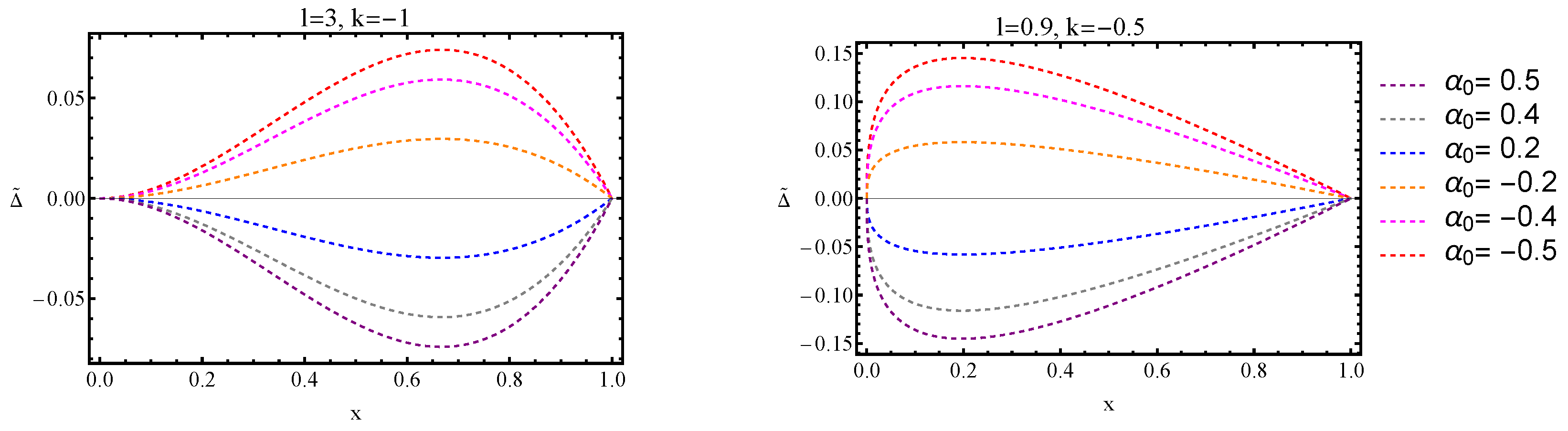
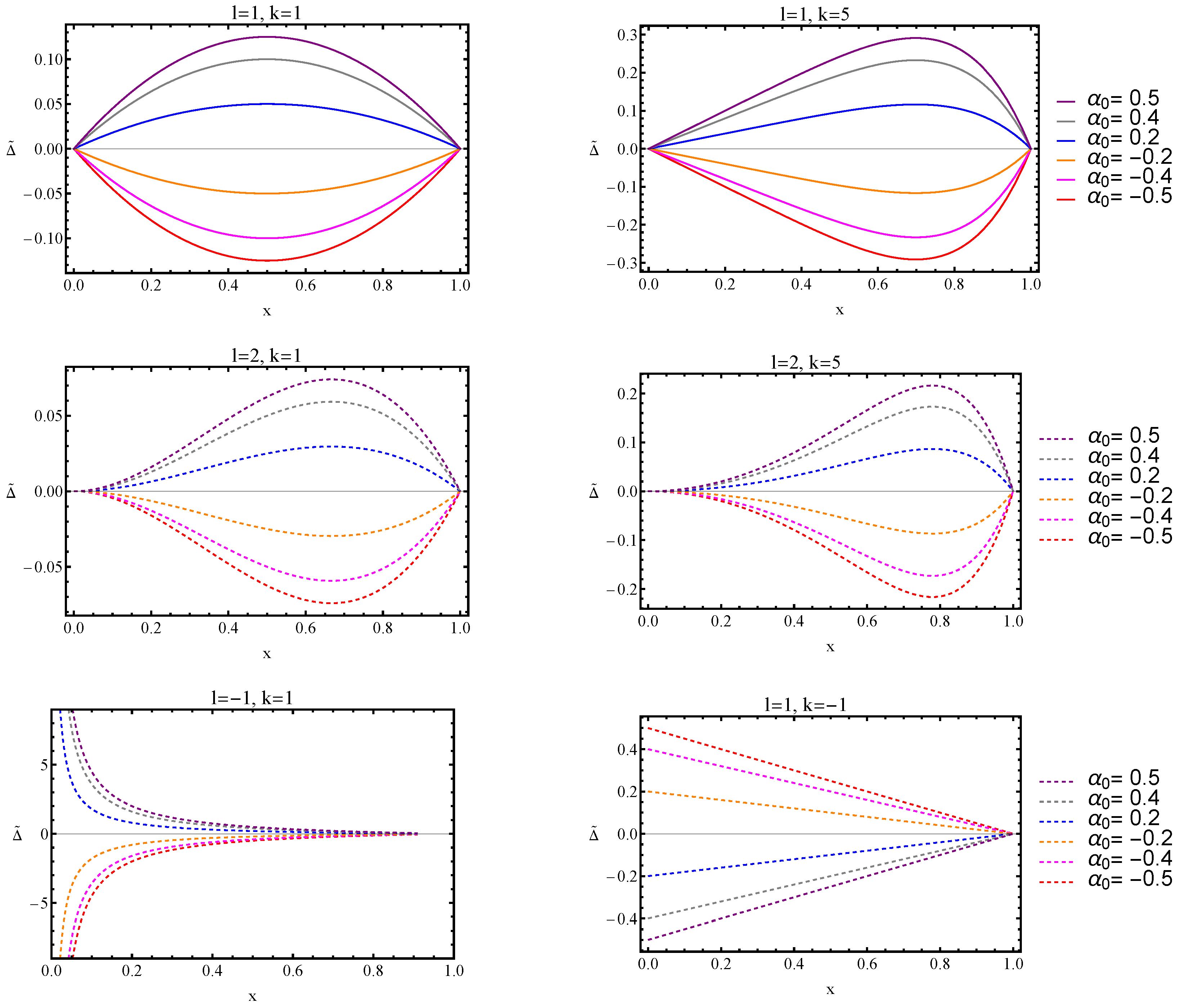
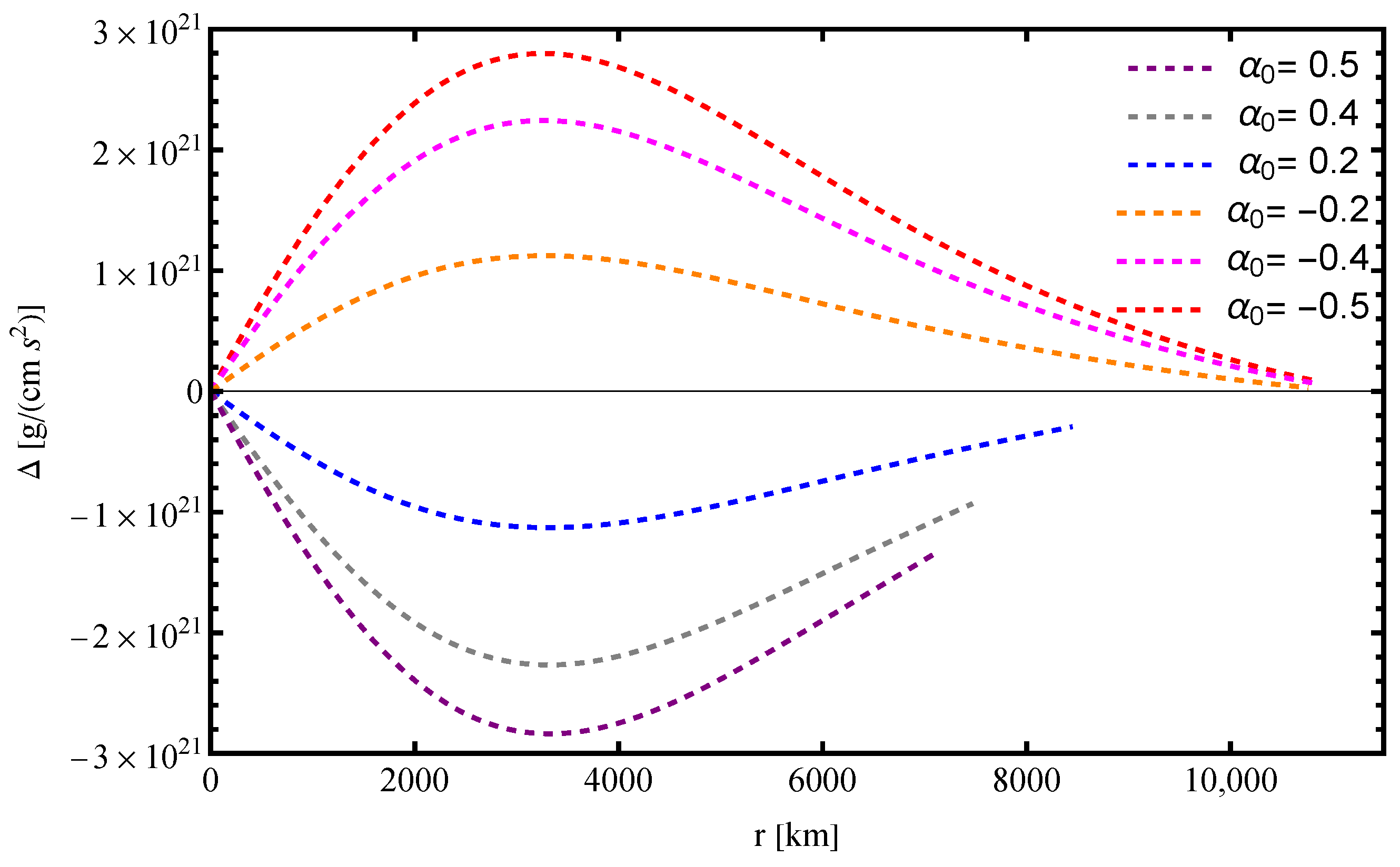
A positive ${\alpha }_0$ results in a negative $\mathsf{\Delta }$, indicating that radial pressure dominates over tangential pressure. Conversely, a negative ${\alpha }_0$ leads to $\mathsf{\Delta }>0$, where tangential pressure becomes dominant.

-

The radial dependence of $\mathsf{\Delta }$ follows a characteristic pattern: it initially grows from zero at the center, reaches a maximum at an intermediate radius, and then diminishes towards the surface. This behavior aligns with expectations for compact stars, where pressure anisotropy is strongest in regions with significant density gradients. The extent of and peak magnitude of anisotropy depend on the choice of ${\alpha }_0$, l, and k, as shown in Figure 7.

-

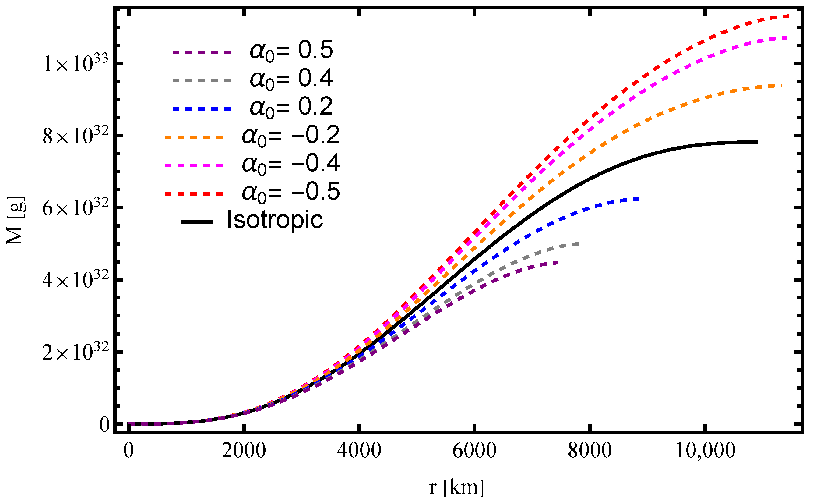
Larger absolute values of ${\alpha }_0$ correspond to stronger deviations between $p_{\perp }$ and $p_{\Vert }$, amplifying the anisotropic effects within the star.

B. Gravitational Redshift

The metric function $\nu \left(r\right)$ is associated with the time–time component of the spacetime metric and determines the gravitational redshift of light emitted from the stellar surface. The surface redshift $z_s$ is given by

$$z_s={\left(1-{\displaystyle \frac{2GM}{c^{2}R}}\right)}^{-1/2}-1={\left(e^{-\nu \left(R\right)}\right)}^{1/2}-1.$$

(46)

This expression links the value of $\nu \left(R\right)$ obtained from the numerical solution to a directly observable quantity: the shift in frequency of photons escaping from the surface of the star. For typical white dwarfs, the redshift is small, usually in the range of ${10}^{-4}$ to ${10}^{-3}$ [71,72,73]. However, in high-density or strongly anisotropic stars, the redshift can become significantly larger and potentially detectable using high-resolution spectroscopy. In this way, the function $\nu \left(r\right)$ provides a meaningful connection between the star’s interior structure and observational data.

To investigate this further, we calculated the surface redshift $z_s$ for each configuration in Table 1. For isotropic models with ${\alpha }_0=0$, the redshift reaches values around $z_s\sim 3.16\times {10}^{-3}$. This value is consistent with typical surface redshifts of massive white dwarfs reported in the literature [72,74]. In anisotropic models with negative ${\alpha }_0$, the redshift decreases noticeably. For example, for ${\alpha }_0=-1$, we find $z_s\sim 0.2\times {10}^{-3}$, which reflects the lower compactness and larger radius of these stars. These results highlight the sensitivity of the redshift to internal pressure anisotropy and suggest that future observations could use this quantity to probe the physical conditions inside white dwarfs.

4.5. Stability Analysis

To examine the compactness and structural stability of the white dwarf, we evaluated the ratio $2M/R$ as a function of the central density ${\rho }_c$ (where ${\rho }_c={10}^n$ g/${\mathrm{cm}}^3$ and n varies from 3 to 12).

The Chandrasekhar limit defines the maximum mass a white dwarf can support before degeneracy pressure becomes insufficient to counteract gravity, leading to a collapse into a neutron star or black hole. The compactness ratio, given by $2M/R$, serves as a key diagnostic for stability. If this ratio approaches the Buchdahl bound ($8/9$) [75], the star becomes unstable against gravitational collapse, indicating a breakdown in hydrostatic equilibrium.

Figure 11 presents the variation of the compactness ratio $2M/R$ as a function of central density ${\rho }_c$. The computed values remain well below the Buchdahl bound, indicating that white dwarfs in this regime maintain hydrostatic equilibrium and do not undergo collapse. Each point in the figure represents a different central density, where the total mass M and radius R are numerically determined. The results confirm that anisotropy does not lead to instability within the considered parameter range.

The structural stability of the anisotropic white dwarf configurations was further examined through the speed of sound condition, which ensures that pressure perturbations propagate at subluminal speeds. The sound speed squared is given by

$$v_s^2={\displaystyle \frac{d{p}_{\Vert }}{d\rho }}.$$

(47)

A physically viable model must satisfy $0\le v_s^2<1$ to ensure causality and stability, preventing superluminal signal propagation and unphysical behavior.

$${\displaystyle \frac{d{p}_{\Vert }}{d\rho }}={\displaystyle \frac{d{p}_{\Vert }}{dr}}{\left({\displaystyle \frac{d\rho }{dr}}\right)}^{-1}=c^2{\displaystyle \frac{d\widetilde{p_{\Vert }}}{dx}}{\left({\displaystyle \frac{d\tilde{\rho }}{dx}}\right)}^{-1},$$

(48)

where the derivatives are obtained from Equation (41) and the differentiation of the dimensionless Equation (29).

Figure 12 presents the variation in $v_s^2$ with radial coordinate r for different values of the anisotropy parameter ${\alpha }_0$. The results demonstrate the following key trends:

-

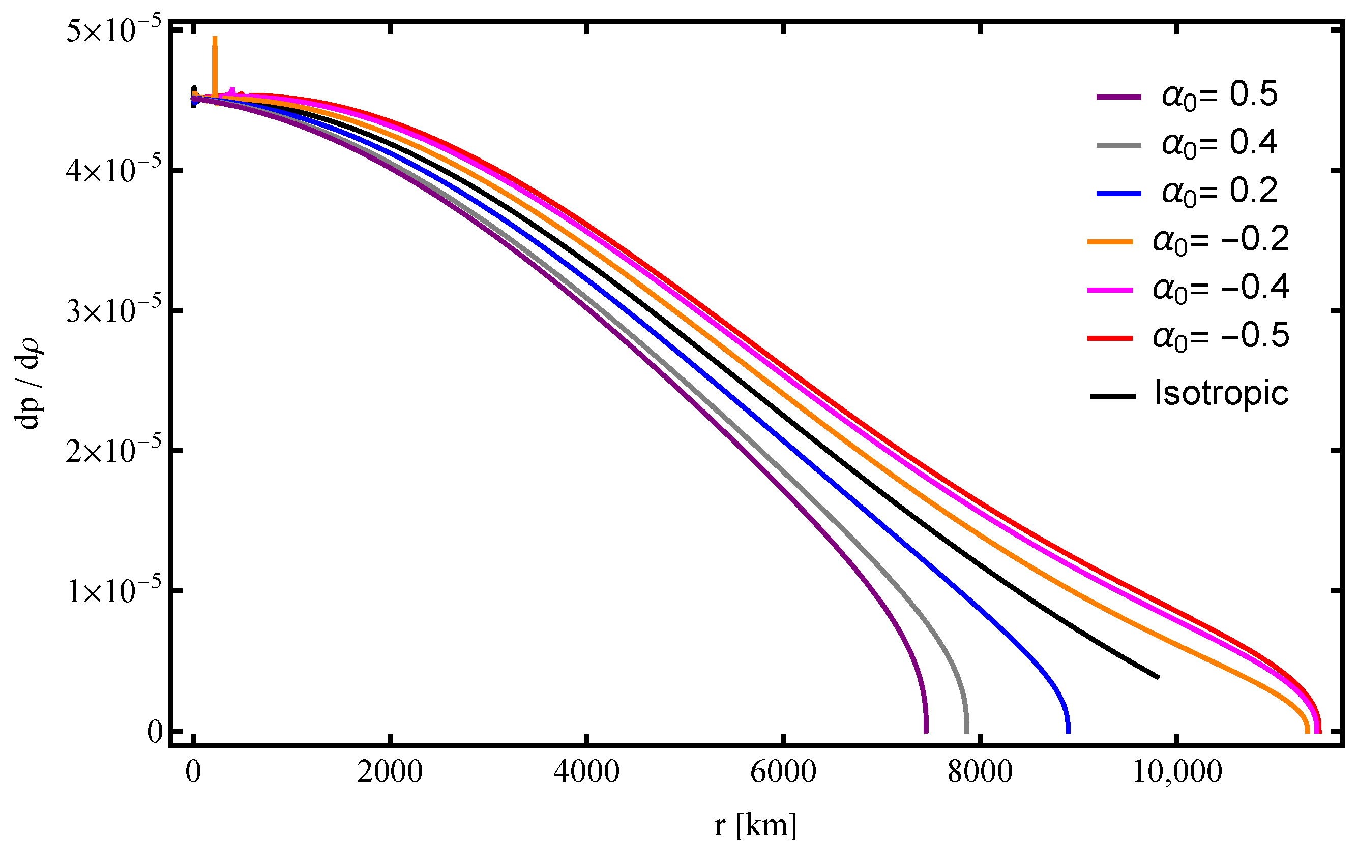
The speed of sound $v_s^2$ remains within the physical bounds across the stellar interior. The sound speed decreases monotonically with increasing radius, which is consistent with expectations for a stable white dwarf. This trend reflects the decreasing pressure gradient toward the surface, where the density is lower.

-

For positive values of ${\alpha }_0$ (e.g., $0.1,0.3,0.5$), $v_s^2$ declines more rapidly, indicating a softer equation of state in the outer layers. Conversely, negative values of ${\alpha }_0$ (e.g., $-0.1,-0.3,-0.5$) correspond to a slower decrease, implying a stiffer equation of state. Despite these variations, the causality condition $v_s^2<1$ is maintained in all cases, confirming the physical viability of the models.

4.6. Sensitivity Analysis

To assess the impact of pressure anisotropy on the equilibrium structure of white dwarfs, we performed a sensitivity analysis by varying the dimensionless anisotropy parameter ${\alpha }_0$ within the physically motivated range $-1\le {\alpha }_0\le 1$. For each selected value of ${\alpha }_0$, equilibrium configurations were computed over a broad range of central densities ${\rho }_c={10}^n\mathrm{g}/{\mathrm{cm}}^3$, where $3\le n\le 12$.

Two types of sensitivity tests were carried out:

(a)

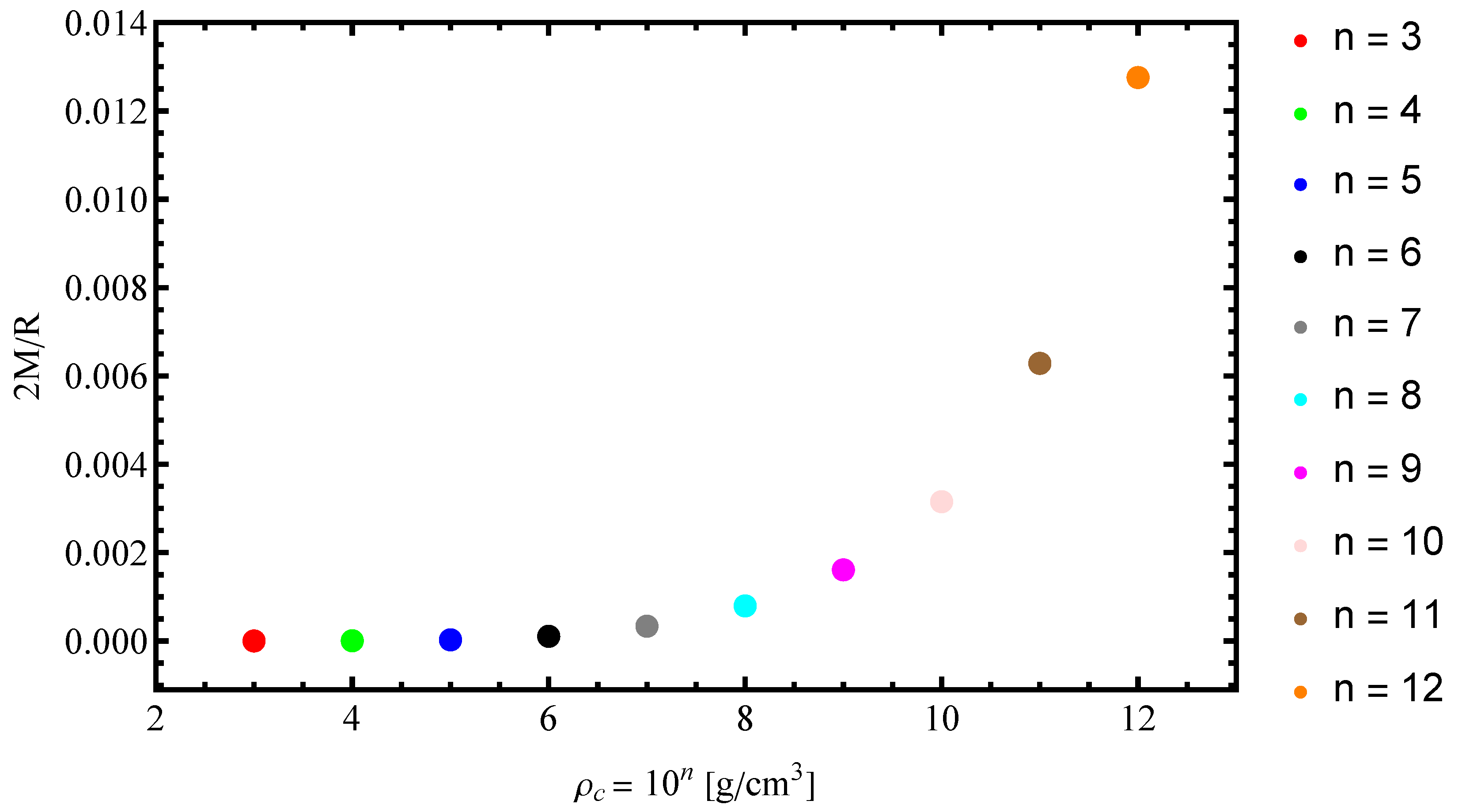
For a fixed ${\alpha }_0$, the central density ${\rho }_c$ was varied to study how structural properties evolve across different density regimes;

(b)

For a fixed central density ${\rho }_c$, the anisotropy parameter ${\alpha }_0$ was varied to examine its influence on stellar mass, radius, and compactness.

For each combination, the modified TOV equations were numerically integrated using the anisotropic pressure term. The results are summarized in Table 1 and

Table 2. Mass, radius, and compactness for various values of ${\alpha }_0$ at a fixed central density ${\rho }_c={10}^{11}\mathrm{g}/{\mathrm{cm}}^3$.

${\mathit{\alpha }}_0$	$(\mathit{R}/{\mathit{R}}_{\odot })\times {10}^{-2}$	$\mathit{M}/{\mathit{M}}_{\odot }$	Compactness $2\mathit{M}/\mathit{R}\times {10}^{-3}$	${\mathit{z}}_{\mathit{s}}\times {10}^{-3}$
$-1$	1.5577	1.44734	0.39349	0.19680
$-0.5$	1.55577	1.41999	0.38653	0.19332
$-0.1$	1.55496	1.39829	0.38082	0.19047
0	0.09385	1.39293	6.28533	3.15756
0.1	0.09384	1.39293	6.28600	3.15789
0.5	0.09382	1.39293	6.28724	3.15852
1	0.09381	1.39293	6.28832	3.15907

.

Negative values of ${\alpha }_0$ result in larger stellar radii and higher masses. Positive values of ${\alpha }_0$ lead to more compact configurations with significantly reduced radii, while the total mass remains nearly constant. This behavior causes compactness to increase for positive ${\alpha }_0$, demonstrating the role of anisotropy in shaping the outer layers of the star.

Table 1 shows that increasing ${\rho }_c$ leads to a monotonic increase in mass and compactness, with the radius slightly decreasing and then stabilizing. For sufficiently high central densities, the mass exceeds the classical Chandrasekhar limit.

For example, at ${\alpha }_0=-1$, the maximum mass reaches $1.447M_{\odot }$. For more negative values such as ${\alpha }_0=-3$, the mass increases to $1.5565M_{\odot }$, significantly above the Chandrasekhar limit. This enhancement results from the dominance of tangential pressure over radial pressure, which provides additional support against gravity.

We do not exclude the possibility that large negative values of the anisotropy parameter (${\alpha }_0<-1$) could substantially affect the global properties of white dwarfs. In particular, the maximum mass may exceed the Chandrasekhar limit by a significant margin. This result aligns with previous investigations suggesting that pronounced anisotropic stresses, originating from mechanisms such as strong magnetic fields, rapid rotation, or unconventional matter interactions, can enhance the mass limits of compact stars beyond those predicted under isotropic assumptions [10,11,12].

Although such configurations are not typical of standard white dwarfs, they may arise in extreme astrophysical environments. In this context, sensitivity analysis provides a valuable framework for probing the extended parameter space of anisotropic stellar models.

Furthermore, the redshift values reported in both tables offer additional insight into the observational implications of anisotropy. As compactness increases with positive values of ${\alpha }_0$, the corresponding surface redshift $z_s$ rises significantly, reaching values up to $z_s\sim 3.16\times {10}^{-3}$ in the most compact configurations. Conversely, for negative ${\alpha }_0$, the redshift remains below $0.2\times {10}^{-3}$, reflecting reduced compactness. These findings suggest that surface redshift measurements may serve as a useful observational tool for identifying or constraining the degree of anisotropy in compact stars.

5. Discussion

The role of anisotropic pressure in white dwarfs was investigated by numerically solving the equilibrium equations using the TOV equation and the Chandrasekhar EoS. The results indicate that anisotropy modifies the internal pressure distribution, leading to systematic deviations in the mass–radius relation compared to isotropic models. Anisotropic effects are most pronounced at intermediate radii but diminish toward the surface, ensuring that the overall equilibrium structure remains consistent with relativistic stellar models. The stability of white dwarfs is preserved, with no indications of large-scale instability.

The structural stability of white dwarf models was assessed using the compactness ratio $2M/R$, which remained well below the Buchdahl bound in all cases. This confirms that moderate anisotropy does not lead to gravitational collapse. The speed of sound criterion further verified that all solutions satisfy causality conditions, ensuring the physical consistency of the models.

The computed mass–radius relation aligns with established results for isotropic models [5,38,64,65]. Previous studies have explored anisotropic pressure effects in various astrophysical contexts, including self-bound stars and relativistic fluids [10,11,12,13]. This study extends these analyses by incorporating a generalized anisotropy framework and evaluating its role in white dwarf stability.

The potential interplay between anisotropic pressure and rotational effects warrants further investigation. Previous studies have demonstrated that, at first order in the quadrupole moment, the gravitational field of a rotating compact object exhibits similar refractive properties to that of a statically deformed source. This suggests that under certain conditions, anisotropic effects may mimic the impact of slow rotation on white dwarf structure and observational signatures such as gravitational lensing and light deflection [16,17,19]. Examining this relationship could provide insights into distinguishing between purely anisotropic and rotationally induced deformations.

Refining the equation of state by incorporating additional microphysical effects, such as Coulomb interactions, magnetic fields, and finite-temperature corrections, could enhance agreement with observational data. Extending this analysis to rotating white dwarfs would provide a more comprehensive understanding of the interplay between anisotropic pressure and rotational deformations. Observational constraints from white dwarf cooling curves and mass–radius measurements could further validate the role of anisotropy in compact star evolution [38,46,76,77]. Analyzing the combined effects of anisotropy, strong magnetic fields, and rapid rotation may provide deeper insights into white dwarf stability and structural properties [78].

In addition to structural modifications, anisotropy may also influence observable quantities such as the surface redshift and thermal evolution of white dwarfs. As discussed in Section 4.4, the metric function $\nu \left(R\right)$ determines the gravitational redshift, which is sensitive to the star’s compactness and, thus, to the degree of anisotropy. Our numerical results in Table 1 show that for isotropic models (${\alpha }_0=0$), the redshift reaches values around $z_s\sim 3.15\times {10}^{-3}$, while for highly anisotropic models with negative ${\alpha }_0$, the redshift drops to $z_s\sim 0.2\times {10}^{-3}$. This trend reflects the decrease in compactness in anisotropic configurations. Since anisotropy modifies the internal pressure and density structure, it may also affect cooling behavior [46]. Future observational data, such as redshift measurements from high-resolution spectroscopy [72,79,80] or observed deviations in white dwarf cooling curves, could help identify and evaluate the presence and strength of pressure anisotropy in real white dwarf populations.

6. Conclusions

This study presented a numerical framework for modeling white dwarfs by solving the field equations coupled with the TOV equations, incorporating anisotropic pressure effects. The introduction of a generalized anisotropic factor provided a systematic approach to analyzing deviations from isotropy and their influence on equilibrium configurations, mass–radius relations, and stability.

Numerical solutions demonstrated that anisotropic pressure alters the internal pressure gradients while preserving hydrostatic equilibrium. The compactness ratio $2M/R$ remained well below the Buchdahl bound, and the speed of sound criterion verified that all models satisfy causality. Sensitivity analysis confirmed the robustness of the results under variations of both the anisotropy parameter ${\alpha }_0$ and central density, reinforcing the reliability of the numerical scheme.

In addition, we computed the gravitational redshift for each configuration and showed that it is sensitive to both compactness and anisotropy. For isotropic models, the redshift reaches values of $z_s\sim 3.15\times {10}^{-3}$, while for anisotropic cases with ${\alpha }_0=-1$, it decreases to $z_s\sim 0.2\times {10}^{-3}$. This variation highlights the potential of redshift measurements as an observational tool to probe pressure anisotropy in compact stars.

We also provided a comparative equation of state (EoS) plot for the Chandrasekhar and Salpeter models, demonstrating that the Salpeter corrections become significant at lower densities. This addition confirms that our numerical framework can accommodate more realistic microphysical inputs, such as electrostatic and Thomas–Fermi effects.

Anisotropic models provide a relevant framework for describing white dwarfs, particularly in astrophysical settings where magnetic fields, strong matter interactions, or rotation may induce deviations from isotropy. Extending this framework to rotating white dwarfs could enhance our understanding of equilibrium structures and stability limits. Future work may also apply this approach to neutron stars and strange stars, contributing to a broader investigation of anisotropic pressure and its role in the structural and dynamical properties of compact astrophysical objects.

References

- Tolman, R.C. Static Solutions of Einstein’s Field Equations for Spheres of Fluid. Phys. Rev. 1939, 55, 364–373. [Google Scholar] [CrossRef]
- Oppenheimer, J.R.; Volkoff, G.M. On Massive Neutron Cores. Phys. Rev. 1939, 55, 374–381. [Google Scholar] [CrossRef]
- Fowler, R.H. On Dense Matter. Mon. Not. R. Astron. Soc. 1926, 87, 114–122. [Google Scholar] [CrossRef]
- Lieb, E.H.; Yau, H.T. The Chandrasekhar theory of stellar collapse as the limit of quantum mechanics. Commun. Math. Phys. 1987, 112, 147–174. [Google Scholar] [CrossRef]
- Chandrasekhar, S. The Maximum Mass of Ideal White Dwarfs. Astrophys. J. 1931, 74, 81. [Google Scholar] [CrossRef]
- Koester, D.; Chanmugam, G. Physics of white dwarf stars. Rep. Prog. Phys. 1990, 53, 837–915. [Google Scholar] [CrossRef]
- Shapiro, S.L.; Teukolsky, S.A. Black Holes, White Dwarfs, and Neutron Stars: The Physics of Compact Objects; Wiley-Interscience: New York, NY, USA, 1983. [Google Scholar]
- Herrera, L.; Santos, N. Local anisotropy in self-gravitating systems. Phys. Rep. 1997, 286, 53–130. [Google Scholar] [CrossRef]
- Giuliani, A.; Rothman, T. Absolute stability limit for relativistic charged spheres. Gen. Relativ. Gravit. 2008, 40, 1427–1447. [Google Scholar] [CrossRef]
- Andréasson, H. Sharp bounds on the critical stability radius for relativistic charged spheres. Commun. Math. Phys. 2009, 288, 715–730. [Google Scholar] [CrossRef]
- Dev, K.; Gleiser, M. Anisotropic stars: Exact solutions. Gen. Relativ. Gravit. 2002, 34, 1793–1818. [Google Scholar] [CrossRef]
- Bowers, R.L.; Liang, E.P.T. Anisotropic Spheres in General Relativity. Astrophys. J. 1974, 188, 657. [Google Scholar] [CrossRef]
- Ivanov, B.V. Maximum bounds on the surface redshift of anisotropic stars. Phys. Rev. D 2002, 65, 104011. [Google Scholar] [CrossRef]
- Zeldovich, Y.B.; Novikov, I.D. Relativistic Astrophysics. Vol.1: Stars and Relativity; University of Chicago Press: Chicago, IL, USA, 1971. [Google Scholar]
- Quevedo, H.; Toktarbay, S. Generating static perfect-fluid solutions of Einstein’s equations. J. Math. Phys. 2015, 56, 052502. [Google Scholar] [CrossRef]
- Toktarbay, S.; Quevedo, H.; Abishev, M.; Muratkhan, A. Gravitational field of slightly deformed naked singularities. Eur. Phys. J. C 2022, 82, 1–8. [Google Scholar] [CrossRef]
- Boshkayev, K.; Quevedo, H.; Toktarbay, S.; Zhami, B.; Abishev, M. On the equivalence of approximate stationary axially symmetric solutions of the Einstein field equations. Gravit. Cosmol. 2016, 22, 305–311. [Google Scholar] [CrossRef]
- Abishev, M.; Beissen, N.; Belissarova, F.; Boshkayev, K.; Mansurova, A.; Muratkhan, A.; Quevedo, H.; Toktarbay, S. Approximate perfect fluid solutions with quadrupole moment. Int. J. Mod. Phys. D 2021, 30, 2150096. [Google Scholar] [CrossRef]
- Beissen, N.; Utepova, D.; Abishev, M.; Quevedo, H.; Khassanov, M.; Toktarbay, S. Gravitational refraction of compact objects with quadrupoles. Symmetry 2023, 15, 614. [Google Scholar] [CrossRef]
- Thorne, K.S.; Misner, C.W.; Wheeler, J.A. Gravitation; Freeman: San Francisco, CA, USA, 2017. [Google Scholar]
- Birkhoff, G.D.; Langer, R.E. Relativity and Modern Physics; Harvard University Press: Cambridge, MA, USA, 1927. [Google Scholar]
- Delgaty, M.; Lake, K. Physical acceptability of isolated, static, spherically symmetric, perfect fluid solutions of Einstein’s equations. Comput. Phys. Commun. 1998, 115, 395–415. [Google Scholar] [CrossRef]
- Landau, L.D. The Classical Theory of Fields; Elsevier: Amsterdam, The Netherlands, 2013; Volume 2. [Google Scholar]
- Weinberg, S. Gravitation and Cosmology: Principles and Applications of the General Theory of Relativity; John Wiley & Sons: Hoboken, NJ, USA, 2013. [Google Scholar]
- Schutz, B. A First Course in General Relativity; Cambridge University Press: Cambridge, UK, 2022. [Google Scholar]
- Cadogan, T.; Poisson, E. Self-gravitating anisotropic fluids. I: Context and overview. Gen. Relativ. Gravit. 2024, 56, 118. [Google Scholar] [CrossRef]
- Duorah, H.; Ray, R. An analytical stellar model. Class. Quantum Gravity 1987, 4, 1691. [Google Scholar] [CrossRef]
- Kepler, S.O.; Pelisoli, I.; Koester, D.; Reindl, N.; Geier, S.; Romero, A.D.; Ourique, G.; Oliveira, C.d.P.; Amaral, L.A. White dwarf and subdwarf stars in the Sloan Digital Sky Survey Data Release 14. Mon. Not. R. Astron. Soc. 2019, 486, 2169–2183. [Google Scholar] [CrossRef]
- Gentile Fusillo, N.P.; Tremblay, P.E.; Gänsicke, B.T.; Manser, C.J.; Cunningham, T.; Cukanovaite, E.; Hollands, M.; Marsh, T.; Raddi, R.; Jordan, S.; et al. A Gaia Data Release 2 catalogue of white dwarfs and a comparison with SDSS. Mon. Not. R. Astron. Soc. 2019, 482, 4570–4591. [Google Scholar] [CrossRef]
- Kilic, M.; Bergeron, P.; Kosakowski, A.; Brown, W.R.; Agüeros, M.A.; Blouin, S. The 100 pc White Dwarf Sample in the SDSS Footprint. Astrophys. J. 2020, 898, 84. [Google Scholar] [CrossRef]
- Boshkayev, K. Equilibrium Configurations of Rotating White Dwarfs at Finite Temperatures. Astron. Rep. 2018, 62, 847–852. [Google Scholar] [CrossRef]
- Miller, M.C.; Lamb, F.K. Observational constraints on neutron star masses and radii. Eur. Phys. J. A 2016, 52, 63. [Google Scholar] [CrossRef]
- Zhao, R.-S.; Yan, Z.; Wu, X.-J.; Shen, Z.-Q.; Manchester, R.N.; Liu, J.; Qiao, G.-J.; Xu, R.-X.; Lee, K.-J. 5.0 GHz TMRT Observations of 71 Pulsars. Astrophys. J. 2019, 874, 64. [Google Scholar] [CrossRef]
- Guillot, S.; Kerr, M.; Ray, P.S.; Bogdanov, S.; Ransom, S.; Deneva, J.S.; Arzoumanian, Z.; Bult, P.; Chakrabarty, D.; Gendreau, K.C.; et al. NICER X-Ray Observations of Seven Nearby Rotation-powered Millisecond Pulsars. Astrophys. J. Lett. 2019, 887, L27. [Google Scholar] [CrossRef]
- Bogdanov, S.; Guillot, S.; Ray, P.S.; Wolff, M.T.; Chakrabarty, D.; Ho, W.C.G.; Kerr, M.; Lamb, F.K.; Lommen, A.; Ludlam, R.M.; et al. Constraining the Neutron Star Mass-Radius Relation and Dense Matter Equation of State with NICER. I. The Millisecond Pulsar X-Ray Data Set. Astrophys. J. 2019, 887, L25. [Google Scholar] [CrossRef]
- Landry, P.; Essick, R.; Chatziioannou, K. Nonparametric constraints on neutron star matter with existing and upcoming gravitational wave and pulsar observations. Phys. Rev. D 2020, 101, 123007. [Google Scholar] [CrossRef]
- Zel’dovich, Y.B.; Novikov, I.D. Theory of Gravitation and the Evolution of Stars; Science: Moscow, Russia, 1971. [Google Scholar]
- Salpeter, E.E. Energy and Pressure of a Zero-Temperature Plasma. Astrophys. J. 1961, 134, 669. [Google Scholar] [CrossRef]
- Takibayev, N.; Kurmangaliyeva, V.; Katō, K.; Vasilevsky, V. Few-Body Reactions and Processes in Neutron Star Envelopes. In Proceedings of the Recent Progress in Few-Body Physics: 22nd International Conference on Few-Body Problems in Physics 22, Caen, France, 9–13 July 2018; Springer: Berlin/Heidelberg, Germany, 2020; pp. 157–161. [Google Scholar]
- Takibayev, N.; Nasirova, D.; Katō, K.; Kurmangaliyeva, V. Excited nuclei, resonances and reactions in neutron star crusts. Proc. J. Phys. Conf. Ser. 2018, 940, 012058. [Google Scholar] [CrossRef]
- Hartle, J.B. Slowly Rotating Relativistic Stars. I. Equations of Structure. Astrophys. J. 1967, 150, 1005. [Google Scholar] [CrossRef]
- Hartle, J.B.; Thorne, K.S. Slowly Rotating Relativistic Stars. III. Static Criterion for Stability. Astrophys. J. 1969, 158, 719. [Google Scholar] [CrossRef]
- Rotondo, M.; Rueda, J.A.; Ruffini, R.; Xue, S.S. Relativistic Feynman-Metropolis-Teller theory for white dwarfs in general relativity. Phys. Rev. D 2011, 84, 084007. [Google Scholar] [CrossRef]
- Chavanis, P.H. Statistical mechanics of self-gravitating systems in general relativity: I. The quantum Fermi gas. Eur. Phys. J. Plus 2020, 135, 290. [Google Scholar] [CrossRef]
- Baiko, D.A.; Yakovlev, D.G. Quantum ion thermodynamics in liquid interiors of white dwarfs. Mon. Not. R. Astron. Soc. 2019, 490, 5839–5847. [Google Scholar] [CrossRef]
- Haensel, P.; Potekhin, A.Y.; Yakovlev, D.G. (Eds.) Neutron Stars 1: Equation of State and Structure; Astrophysics and Space Science Library; Springer: New York, NY, USA, 2007; Volume 326. [Google Scholar]
- de Carvalho, S.M.; Rotondo, M.; Rueda, J.A.; Ruffini, R. Relativistic Feynman-Metropolis-Teller treatment at finite temperatures. Phys. Rev. C 2014, 89, 015801. [Google Scholar] [CrossRef]
- Bauswein, A.; Blacker, S.; Vijayan, V.; Stergioulas, N.; Chatziioannou, K.; Clark, J.A.; Bastian, N.-U.F.; Blaschke, D.B.; Cierniak, M.; Fischer, T.; et al. Equation of State Constraints from the Threshold Binary Mass for Prompt Collapse of Neutron Star Mergers. Phys. Rev. Lett. 2020, 125, 141103. [Google Scholar] [CrossRef]
- Boshkayev, K.A.; Rueda, J.A.; Zhami, B.A.; Kalymova, Z.A.; Balgymbekov, G.S. Equilibrium structure of white dwarfs at finite temperatures. Proc. Int. J. Mod. Phys. Conf. Ser. 2016, 41, 1660129. [Google Scholar] [CrossRef]
- Boshkayev, K.; Rueda, J.A.; Ruffini, R.; Zhami, B.; Kalymova, Z.; Balgimbekov, G. Mass-radius relations of white dwarfs at finite temperatures. In Proceedings of the 14th Marcel Grossmann Meeting on Recent Developments in Theoretical and Experimental General Relativity, Astrophysics, and Relativistic Field Theories, Rome, Italy, 12–18 July 2015. [Google Scholar]
- Faussurier, G. Relativistic finite-temperature Thomas-Fermi model. Phys. Plasmas 2017, 24, 112901. [Google Scholar] [CrossRef]
- Fantoni, R. White-dwarf equation of state and structure: The effect of temperature. J. Stat. Mech. Theory Exp. 2017, 11, 113101. [Google Scholar] [CrossRef]
- Belvedere, R.; Boshkayev, K.; Rueda, J.A.; Ruffini, R. Uniformly rotating neutron stars in the global and local charge neutrality cases. Nucl. Phys. A 2014, 921, 33–59. [Google Scholar] [CrossRef]
- Raithel, C. Constraining the Neutron Star Equation of State with Gravitational Wave Events. In Proceedings of the Constraining the Neutron Star Equation of State with Gravitational Wave, Honolulu, HI, USA, 4–8 January 2020. American Astronomical Society Meeting Abstracts #237.03. [Google Scholar]
- Raaijmakers, G.; Greif, S.K.; Riley, T.E.; Hinderer, T.; Hebeler, K.; Schwenk, A.; Watts, A.L.; Nissanke, S.; Guillot, S.; Lattimer, J.M.; et al. Constraining the dense matter equation of state with joint analysis of NICER and LIGO/Virgo measurements. Astrophys. J. Lett. 2020, 893, L21. [Google Scholar] [CrossRef]
- Burgio, G.F.; Vidana, I. The Equation of State of Nuclear Matter: From Finite Nuclei to Neutron Stars. Universe 2020, 6, 119. [Google Scholar] [CrossRef]
- Chatziioannou, K. Neutron star tidal deformability and equation of state constraints. Gen. Relativ. Gravit. 2020, 52, 109. [Google Scholar] [CrossRef]
- Pretel, J.M.Z.; da Silva, M.F.A. Stability and gravitational collapse of neutron stars with realistic equations of state. Mon. Not. R. Astron. Soc. 2020, 495, 5027–5039. [Google Scholar] [CrossRef]
- Greif, S.K.; Hebeler, K.; Lattimer, J.M.; Pethick, C.J.; Schwenk, A. Equation of state constraints from nuclear physics, neutron star masses, and future moment of inertia measurements. Astrophys. J. 2020, 901, 155. [Google Scholar] [CrossRef]
- Drischler, C.; Furnstahl, R.J.; Melendez, J.A.; Phillips, D.R. How Well Do We Know the Neutron-Matter Equation of State at the Densities Inside Neutron Stars? A Bayesian Approach with Correlated Uncertainties. Phys. Rev. Lett. 2020, 125, 202702. [Google Scholar] [CrossRef]
- Demorest, P.B.; Pennucci, T.; Ransom, S.M.; Roberts, M.S.E.; Hessels, J.W.T. A two-solar-mass neutron star measured using Shapiro delay. Nature 2010, 467, 1081–1083. [Google Scholar] [CrossRef]
- Antoniadis, J.; Freire, P.C.C.; Wex, N.; Tauris, T.M.; Lynch, R.S.; Van Kerkwijk, M.H.; Kramer, M.; Bassa, C.; Dhillon, V.S.; Driebe, T.; et al. A Massive Pulsar in a Compact Relativistic Binary. Science 2013, 340, 1233232. [Google Scholar] [CrossRef]
- Boshkayev, K.; Zhami, B.; Kalymova, Z.A.; Balgimbekov, G.S.; Taukenova, A.; Brisheva, Z.N.; Koyshybaev, N. Theoretical Calculation of the Main Parameters of White Dwarf Stars. Phys.-Math. Ser. 2016, 3, 49–60. [Google Scholar]
- Koester, D.; Reimers, D. White dwarfs in open clusters. VIII. NGC 2516: A test for the mass-radius and initial-final mass relations. Astron. Astrophys. 1996, 313, 810–814. [Google Scholar]
- Panei, J.; Althaus, L.; Benvenuto, O. Mass-radius relations for white dwarf stars of different internal compositions. arXiv 1999, arXiv:astro-ph/9909499. [Google Scholar]
- Kumar, J.; Bharti, P. Relativistic models for anisotropic compact stars: A review. New Astron. Rev. 2022, 95, 101662. [Google Scholar] [CrossRef]
- Cadogan, T.; Poisson, E. Self-gravitating anisotropic fluid. II: Newtonian theory. Gen. Relativ. Gravit. 2024, 56, 119. [Google Scholar] [CrossRef]
- Cadogan, T.; Poisson, E. Self-gravitating anisotropic fluid. III: Relativistic theory. Gen. Relativ. Gravit. 2024, 56, 120. [Google Scholar] [CrossRef]
- Dev, K.; Gleiser, M. Anisotropic stars II: Stability. Gen. Relativ. Gravit. 2003, 35, 1435–1457. [Google Scholar] [CrossRef]
- Maurya, S.; Ratanpal, B.; Govender, M. Anisotropic stars for spherically symmetric spacetimes satisfying the Karmarkar condition. Ann. Phys. 2017, 382, 36–49. [Google Scholar] [CrossRef]
- Barstow, M.A.; Bond, H.E.; Holberg, J.B.; Burleigh, M.R.; Hubeny, I.; Koester, D. Hubble Space Telescope spectroscopy of the Balmer lines in Sirius B★. Mon. Not. R. Astron. Soc. 2005, 362, 1134–1142. [Google Scholar] [CrossRef]
- Bond, H.E.; Schaefer, G.H.; Gilliland, R.L.; Holberg, J.B.; Mason, B.D.; Lindenblad, I.W.; Seitz-McLeese, M.; Arnett, W.D.; Demarque, P.; Spada, F.; et al. The Sirius System and Its Astrophysical Puzzles: Hubble Space Telescope and Ground-based Astrometry*. Astrophys. J. 2017, 840, 70. [Google Scholar] [CrossRef]
- Joyce, S.R.G.; Barstow, M.A.; Holberg, J.B.; Bond, H.E.; Casewell, S.L.; Burleigh, M.R. The gravitational redshift of Sirius B. Mon. Not. R. Astron. Soc. 2018, 481, 2361–2370. [Google Scholar] [CrossRef]
- Koester, D. White Dwarfs: Recent Results and Open Problems. Astrophys. Space Sci. 1987, 131, 351–364. [Google Scholar] [CrossRef]
- Buchdahl, H.A. General Relativistic Fluid Spheres. Phys. Rev. 1959, 116, 1027–1034. [Google Scholar] [CrossRef]
- Boshkayev, K.; Rueda, J.A.; Ruffini, R.; Siutsou, I. On general relativistic uniformly rotating white dwarfs. Astrophys. J. 2012, 762, 117. [Google Scholar] [CrossRef]
- Chabrier, G.; Potekhin, A.Y. Equation of state of fully ionized electron-ion plasmas. Phys. Rev. E 1998, 58, 4941. [Google Scholar] [CrossRef]
- Cardall, C.Y.; Prakash, M.; Lattimer, J.M. Effects of strong magnetic fields on neutron StarStructure. Astrophys. J. 2001, 554, 322. [Google Scholar] [CrossRef]
- Bédard, A.; Bergeron, P.; Fontaine, G.; Billères, M. A Gaia Data Release 2 White Dwarf Mass Distribution: The Need for a Revised Mass-Radius Relation. Astrophys. J. 2020, 901, 93. [Google Scholar] [CrossRef]
- Gentile Fusillo, N.P.; Tremblay, P.E.; Cukanovaite, E.; Vorontseva, A.; Lallement, R.; Hollands, M.; Gänsicke, B.T.; Burdge, K.B.; McCleery, J.; Jordan, S. A Gaia catalogue of white dwarfs I: DA white dwarfs from Gaia EDR3. Mon. Not. R. Astron. Soc. 2021, 508, 3877–3896. [Google Scholar] [CrossRef]