Properties of MAXI J1348-630 during Its Second Outburst in 2019

Abstract

The newly discovered galactic black hole candidate (BHC) MAXI J1348-630 showed two major outbursts in 2019, just after its discovery. Here, we provide a detailed spectral and temporal analysis of the less-studied second outburst using archive data from multiple satellites, namely Swift, MAXI, NICER, NuSTAR and AstroSat. The outburst continued for around two and a half months. Unlike the first outburst from this source, this second outburst was a ‘failed’ one. The source did not transition to soft or intermediate spectral states. During the entire outburst, the source was in the hard state with high dominance of non-thermal photons. The presence of strong shocks are inferred from spectral fitting using a TCAF model. In NuSTAR spectra, weak reflection is observed from spectral fitting. Low-frequency quasi-periodic oscillations are also detected in AstroSat data.

1. Introduction

Black hole X-ray binaries are one of the most interesting astronomical objects as they show rapid variability in timing and spectral properties. A black hole X-ray binary system consists of a black hole (BH) and a companion star. At some later stage during evolution, the companion star fills its Roche lobe and, due to the immense gravitational pull of the BH, mass from the companion starts to accrete towards the black hole through the Lagrangian point L1 [1]. This process is known as the Roche lobe overflow. There may also be wind accretion and tidal deformation. Matter accretes to the BH after forming a spirally rotating accretion disk around the BH. BHs can be explored by detecting the electromagnetic radiation coming out from the accretion disk around them. The gravitational potential energy of the accreting matter is converted into energy that is radiated over the entire electromagnetic wave band (from radio to $\gamma$-ray).

Stellar mass black hole X-ray binaries can be classified as either transient or persistent. Persistent sources always remain in the active phase, whereas transient sources mostly remain in the quiescent phase and occasionally have outbursts. In the case of transient sources, viscosity plays a major role in triggering an outburst. The inflowing matter from the companion initially accumulates at the ‘pile-up’ radius [2,3,4], and when the viscosity increases and exceeds the critical limit, the accumulated matter starts to accrete and triggers an outburst. The outbursts of X-ray novae can be well-explained by the hydrogen instability model [5,6,7]. In the case of low-mass X-ray binaries, the hydrogen ionization instability operating in an accretion disk can describe the shape of outburst light curves [8,9].

An outbursting BH generally goes through four spectral states: low hard state (LHS) or hard state (HS), hard intermediate state (HIMS), soft intermediate state (SIMS) and soft state (SS) or high soft state (HSS) [10,11,12]. Evolution of states can be observed through a hardness intensity diagram (HID) or “q” diagram [13,14] and an accretion-rate ratio intensity diagram [15,16]. A BH is observed with low luminosity in the HS at the beginning of an outburst. As time passes, luminosity increases and the BH moves towards the SS via HIMS and SIMS. In SS, the luminosity remains very high. After that, the source enters the declining phase and moves to the HS through SIMS and HIMS. In short, the BH evolves through the four canonical spectral states, forming a hysteresis loop in the sequence: HS (rising) → HIMS (rising) → SIMS (rising) → SS → SIMS (declining) → HIMS (declining) → HS (declining). An outburst can be classified as normal or failed, depending on its spectral variation [17]. Normal outbursts evolve through all the spectral states and are complete in nature. Failed outbursts do not show softer spectral states (SIMS and SS). Normal outbursts are sometimes defined as ‘successsful’ outbursts, and failed outbursts are ‘hard-only’ outbursts [18].

Generally, the energy spectrum of a BH consists of two components: a multi-color thermal black body or disk black body (DBB) and a non-thermal powerlaw (PL). Non-thermal, high-energy radiation dominates the harder states (HS and HIMS), and thermal black body radiation dominates the softer states (SIMS and SS). Multi-color black body emission originates in the standard disk [19,20], and powerlaw emission originates in a Compton cloud consisting of hot electrons [21,22]. Various models are present in the literature to understand and explain the accretion properties of black holes, such as Bondi flow [23], standard disk model [20], thick disk model [24] and ADAF model [25]. These models can explain the radiation spectra of black holes to some extent. In the mid 1990s, Chakrabarti and his collaborators came up with the Two Component Advective Flow (TCAF) solution based on transonic flow and radiative transport equations [26,27,28]. In this model, the accretion flow consists of two components: a geometrically thin, optically thick, high-viscosity Keplerian disk, and a low-viscosity, optically thin, sub-Keplerian flow or halo. The Keplerian matter accretes on the equatorial plane and is immersed within the sub-Keplerian flow. The sub-Keplerian flow (halo) moves in freefall timescale, and it moves faster than the Keplerian matter moving in a viscous timescale. The sub-Keplerian flow temporarily slows down at the centrifugal barrier and forms an axisymmetric shock [29]. The post-shock region is hot and puffed-up and is known as the CENtrifugal pressure supported BOundary Layer (CENBOL). The CENBOL acts as a Compton cloud in the TCAF solution. Multi-color black body spectra are generated from the soft photons originating in the Keplerian disk. A fraction of these soft photons (from the Keplerian disk) are intercepted by the CENBOL and are inverse-Comptonized by highly energetic ‘hot’ electrons of the CENBOL to produce hard photons. The powerlaw tail in the spectra is produced by these hard photons. Part of the hard photons interact with the Keplerian disk, and for this reason a ‘reflection hump’ is observed at high energy.

The TCAF model has been implemented as an additive table model in XSPEC to obtain direct estimation of flow parameters and mass of the BH from spectral fitting [30]. This model has four basic flow parameters: (i) Keplerian disk rate (${\dot{m}}_d$ in ${\dot{M}}_{Edd}$), (ii) sub-Keplerian halo rate (${\dot{m}}_h$ in ${\dot{M}}_{Edd}$), (iii) shock location ($X_s$ in Schwarzschild radius $r_s$), i.e., the boundary of CENBOL, and (iv) compression ratio (R), i.e., the ratio of the pre-shock matter density to the post-shock matter density and two other parameters: mass of the BH ($M_{BH}$ in $M_{\odot }$) and normalization (N). From recent studies by our group, we can claim that the TCAF model is quite successful for explaining the physics around compact objects. Accretion flow dynamics of black hole candidates (BHCs) can be understood more clearly from the analysis of more than fifteen BHCs [15,16,30,31,32,33,34,35,36] using the TCAF model. The mass of BHCs has also been estimated from spectral analysis using the TCAF model [37,38,39,40].

In BHs, jets/outflows are very important phenomena. In astrophysical jets, mass, energy and angular momentum are channeled as a beam of ionized matter along the axis of rotation. Jets from compact objects are geometrically narrow and conical in shape. In HS, collimated and compact jets are observed, whereas in intermediate states (HIMS and SIMS), jets are observed as discrete and blobby in nature. The contribution of the jet component to the total observed X-ray flux can be estimated from spectral analysis with the TCAF model [41,42]. Generally, no jets are observed in SS. However, there can also be jets in SS for magnetically dominated accretion disks [42]. The precise mechanism of the production of jets is still unknown. Though jets are widely observed, the reasons behind their creation, collimation and acceleration are still up for debate. Several theories have been proposed in the literature to explain jets and outflows, such as de-Laval nozzles [43], an electrodynamical acceleration model [44] and self-similar centrifugally driven outflows [45]. Blandford and Znajek 1977 [46] made one of the earliest models for jet solutions. The Blandford–Znajek process describes how jet power is extracted from the spin energy of the black hole. A jet will be visible in all spectral states if it is driven by spin energy. However, in reality, jets are not observed in the soft spectral state. Generally, it is thought that the magnetic field causes jets to collide [47]. According to Chakrabarti and Bhaskaran 1992 [48], jets or outflows are ejected, accelerated and collimated by hydromagnetic processes. In the TCAF model, the CENBOL acts as the base of the jets. Here, radiation pressure is responsible for launching the jet [49].

BHs exhibit quasi-periodic oscillations (QPOs) in some spectral states. Low-frequency QPOs (LFQPOs) are very common observable features in the power density spectrum (PDS) of stellar mass BHs. A few BHs show high-frequency QPOs in their PDSs. These X-ray transient sources exhibit QPOs with frequencies ranging from mHz to a few hundred Hz [50]. Many scientific groups have reported low- (~0.01–30 Hz) as well as high- (~40–450 Hz) frequency QPOs in black hole X-ray binaries (BHXRBs) (for a review see [10,12] and references therein). Depending on their nature (Q value, RMS amplitude, noise, etc.), LFQPOs can be divided into three types: type-A, type-B and type-C [51,52]. In HS and HIMS, type-C QPOs can be seen. In SIMS, type-A or type-B QPOs are observed. Generally QPOs are not observed in SS. The origin of the QPOs can be described as the oscillation of the CENBOL in the TCAF model [30,33,53,54]. When the radiative cooling timescale and the infall timescale roughly match, the outer boundary of the CENBOL oscillates, and the emerging photons produce QPOs [54,55,56]. QPOs are also observed if Rankine–Hugoniot conditions for the stable shock are not satisfied [56].

The Galactic BHC MAXI J1348-630 was discovered on 26 January 2019 by the gas slit camera (GSC) onboard Monitor of All-sky X-ray Image (MAXI) [57,58], and based on its estimated mass and spectral features, it was classified as a BH binary [59]. Swift/XRT observation localized the source at R.A. = ${13}^h$48${}^{\prime }$12.73${}^{″}$, Decl. = $-{63}^{\circ }$16${}^{\prime }$26.8${}^{″}$ [60]. The source was also observed by several X-ray observatories, such as INTEGRAL, NICER, Insight-HXMT, AstroSat, Swift and NuSTAR [61,62,63]. After completion of the first outburst, there was a quiescence of ~20 days, and the source again re-brightened and started a new outburst that lasted for two and a half months from MJD ~ 58,630 to MJD ~ 58,700. After completion of this second large outburst, six mini outbursts were detected during the centroid time of MJD ~ 58,747.6 ± 0.4, MJD ~ 58,812.7 ± 0.3, MJD ~ 58,886.8 ± 0.4, MJD ~ 58,975.8 ± 1.0, MJD ~ 59,033.3 ± 1.6 and MJD 59,098.0 [64,65,66].

The first outburst lasted for four months, and the source showed all four canonical spectral states. A detailed study of the spectral evolution of the first outburst was performed with MAXI [39,59], Swift [39,67] and Insight-HXMT [67]. Chauhan et al. (2020) [68] estimated the most-probable distance of MAXI J1348-630 as ${2.2}_{-0.6}^{+0.5}$ kpc. Based on spectral analysis, Tominaga et al. (2020) [59] predicted that MAXI J1348-630 hosts a relatively massive black hole and reported a range of mass of the BH dependent on different spinning parameters and inclination angles. However, Jana et al., 2020 [39], estimated the mass of the BH as ${9.1}_{-1.2}^{+1.8}$$M_{\odot }$ from spectral analysis with the physically motivated TCAF model. The spin parameter was estimated as $a={0.78}_{-0.04}^{+0.04}$, and the inclination angle of the inner disc was estimated to be $i={29.2}_{-0.5}^{+0.3}$ from reflection spectroscopy using NuSTAR observations [69]. The reflection was found to be from a high-density accretion disk [70]. During the first outburst, type-B QPO was observed from NICER observations [71,72]. A time lag between different energy bands was observed during the first outburst [73].

Although the first outburst of MAXI J1348-630 has been studied extensively, the second outburst has not been studied in detail. In this paper, we study the evolution of the spectral and timing properties of the second outburst in detail using data obtained from Swift, MAXI, NICER, NuSTAR and AstroSat observatories. The paper is organized as follows. In Section 2 and Section 3, we discuss data reduction and analysis methods, respectively. In Section 4, we present our results. In Section 5, we discuss findings and draw our conclusions.

2. Data Reduction

We studied the BHC MAXI J1348-630 during its second outburst (2019 May to 2019 August). The outburst continued for two and a half months. In our analysis, we used the data from Swift, NICER, NuSTAR and MAXI for spectral analysis. A total of 21 observations were used for the spectral study. Out of these 21 observations, 8 are combined Swift/XRT and MAXI/GSC, 2 are Swift/XRT-only, 8 are combined NICER and MAXI/GSC, and 3 are NuSTAR-only (check

Table 1. Log of Swift, NICER and NuSTAR observations of the transient BHC MAXI J1348-630.

ID	Obs. ID	Satellite/Instrument	MJD	Date of Obs.	Exposure
				YYYY-MM-DD	(ks)
(1)	(2)	(3)	(4)	(5)	(6)
X1	00011107040	XRT+GSC	58,630.70	2019-05-27	1.02
X2	00011107041	XRT+GSC	58,633.39	2019-05-30	0.86
X3	00011107042	XRT+GSC	58,639.67	2019-06-05	1.00
X4	00011107043	XRT+GSC	58,647.82	2019-06-13	1.07
X5	00011107044	XRT+GSC	58,650.84	2019-06-16	1.00
X6	00011107045	XRT	58,685.02	2019-07-21	0.93
X7	00011107046	XRT+GSC	58,689.63	2019-07-25	2.01
X8	00011107047	XRT+GSC	58,690.23	2019-07-26	1.60
X9	00011107048	XRT	58,699.84	2019-08-04	1.00
X10	00011107049	XRT+GSC	58,706.42	2019-08-11	0.90
NI1	2200530143	NICER+GSC	58,634.04	2019-05-31	1.37
NI2	2200530144	NICER+GSC	58,637.81	2019-06-03	1.11
NI3	2200530170	NICER+GSC	58,675.91	2019-07-11	0.49
NI4	2200530172	NICER+GSC	58,678.44	2019-07-14	1.35
NI5	2200530175	NICER+GSC	58,681.43	2019-07-17	1.23
NI6	2200530185	NICER+GSC	58,691.62	2019-07-27	1.70
NI7	2200530187	NICER+GSC	58,693.49	2019-07-29	0.78
NI8	2200530190	NICER+GSC	58,696.14	2019-08-01	0.71
NU1	80502304002	NuSTAR	58,655.60	2019-06-21	13.78
NU2	80502304004	NuSTAR	58,660.73	2019-06-26	15.37
NU3	80502304006	NuSTAR	58,672.61	2019-07-08	17.18

). Furthermore, for timing analysis, we used AstroSat/LAXPC and NICER data.

2.1. Swift/XRT

First, we used the XRTPIPWLINE 1 command to generate cleaned level-2 event files from the level-1 data files. Using the XSELECT task, a circular region of radius 30 arcseconds was chosen around the source location to generate the source region file. We also chose a background region of radius 30 arcseconds away from the source to produce the background region file. Using the region files, we extracted spectra for both the source and the background. With the help of the tool XRTMKARF, we created corresponding ARFs. We obtained the appropriate RMFs from the CALDB. Using the grppha task, we re-binned the spectra with a minimum of 20 counts/bin.

2.2. NICER

NICER has unprecedented spectral and timing resolutions of ~85 eV at 1 keV and ~100 nanoseconds, respectively. We used the latest calibration files (20210707) for data reduction. To analyze the NICER data, we first processed the data with the NICERL2 script, which runs a standard pipeline and produces cleaned level-2 event files with the use of standard calibration. Then, we ran the command barycorr to produce the barycenter-corrected cleaned event file. The barycentered-corrected cleaned event files were used to extract the light curve and spectrum in the XSELECT environment. The nibackgen3C50 tool was used to produce the background spectra corresponding to each of the observation IDs. The spectra were re-binned with a minimum of 20 counts per bin with the use of grppha. To search for QPOs, we extracted the 0.01 s binned light curves from the barycenter-corrected cleaned event file using xselect.

2.3. NuSTAR

We used NuSTAR/FPMA data in the 4–78 keV energy band to get broad energy information. Data reduction was done using the NuSTAR data analysis software NUSTARDAS. First, the NUPIPELINE command was run to get the stage-II data for the Focal Plane Module FPMA. A circular region of 80 arcseconds was chosen at the source location to generate the source region file. We also chose a region of 80 arcseconds away from the source to generate the background region file. We generated spectra, RMF and ARF files using nuproduct. The extracted spectra were re-binned to have at least 30 counts per bin with the tool grppha.

2.4. MAXI/GSC

We used the MAXI on-demand process web tool to generate 6–20 keV MAXI/GSC spectra using the process mentioned in Matsuoka et al., 2009 [58]. The MAXI/GSC spectrum files are available from (http://maxi.riken.jp/mxondem, accessed on 15 January 2022). We downloaded the MAXI/GSC spectral observations that were simultaneous/quasi-simultaneous with those of XRT and NICER. One-day-averaged light curves in different energy ranges available from (http://maxi.riken.jp/top/lc.html, accessed on 11 January 2022) were used to observe the variation of flux.

2.5. AstroSat/LAXPC

We used publicly available code from the LAXPC Software website to produce cleaned level-2 data from the level-1 data files from LAXPC20. For each observation, we initially ran the ‘laxpcl1.f’ program to process multiple orbits of level-1 data. This program outputs event files, light curves, spectra and GTI files in both ASCII and FITS formats. Then, the ‘backshiftv3.f’ program was used to apply background correction to the light curve files. For each observation, we initially ran the program ‘laxpcl1.f’ with a time bin of 1 s and the full range of anodes and channels. The program produced output files along with the lxp1level2.gti, which was moved to the file gti.inp. Once the gti.inp file was prepared, we extracted the 0.01 s binned light curve by running the program ‘laxpcl1.f’ again with the full range of anodes and channels. We used the 0.01 s time binned light curves (3–80 keV) to search for the QPOs.

3. Data Analysis

3.1. Temporal Analysis

Archival data from MAXI/GSC2 (2–10 keV) and SWIFT/BAT3 (15–50 keV) were used to observe the variation of fluxes during the outburst. The one-day-averaged light curves were converted into $Crab$ units using proper conversion factors. The Crab conversion factor for GSC (2–10 keV) data is 2.82 photons cm⁻² s⁻¹, and for BAT, the Crab conversion factor is 0.218 counts cm⁻² s⁻¹. To search for the QPOs, we generated the white-noise-subtracted power density spectra (PDS) using 0.01 s time binned light curves of AstroSat (3–80 keV) and NICER (1–10 keV) data. The powspec task of the XRONOS software package was used to generate the PDS from the 0.01 s time binned light curves. Each light curve was divided into 8192 intervals, and a PDS for each interval was generated; these were normalized so that their integral gave the squared rms fractional variability. To obtain the final PDS, all individual PDSs were then averaged. We used geometrical re-binning constants of $-1.02$ or $-1.05$ as needed on the final PDSs. We used a multiple Lorentzian model to fit the PDS. From this, we obtained the fitted values of QPO frequencies (${\nu }_{QPO}$), width ($\Delta \nu$), Q-value ($Q={\nu }_{QPO}/\Delta \nu$) and RMS (%) amplitude. With the help of these values, we classified the nature of the QPOs.

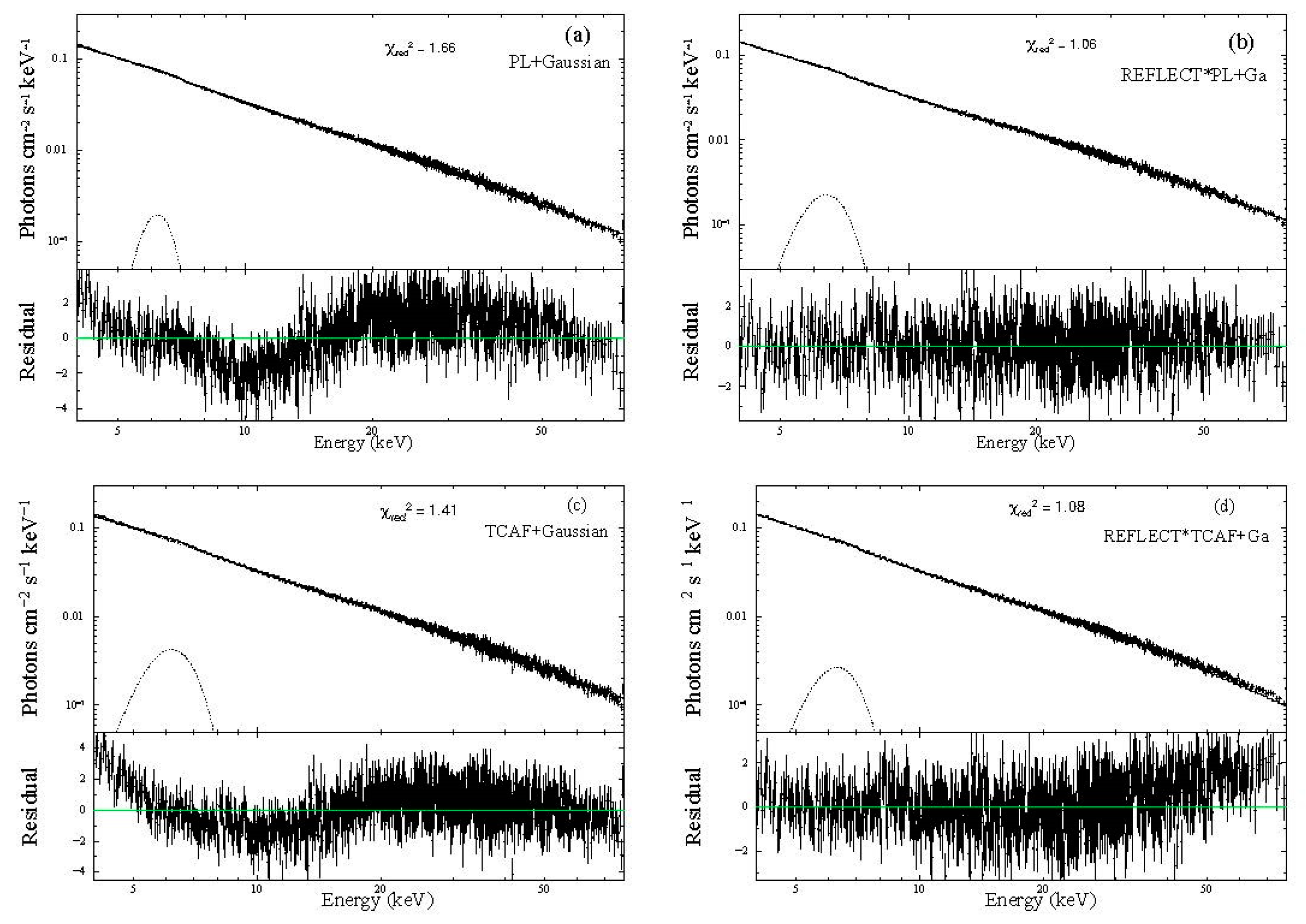
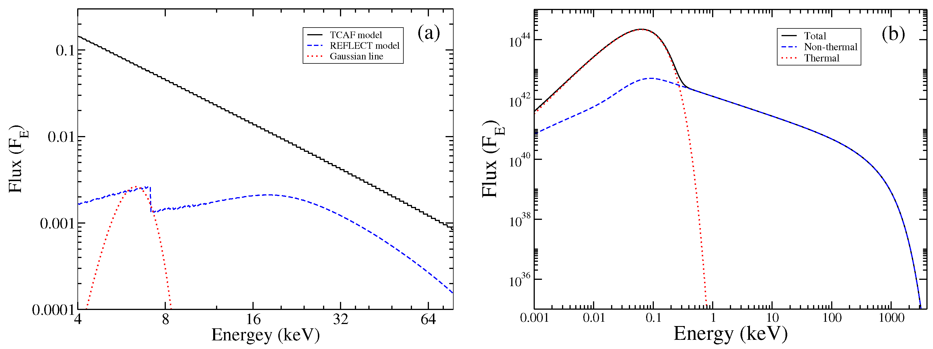
3.2. Spectral Analysis

  For spectral analysis, we used XRT spectra from 1–8 keV, GSC from 6–20 keV, NICER from 1–10 keV and NuSTAR from 4–78 keV energy ranges. For our spectral study, we used 21 total observations. We analyzed simultaneous/quasi-simultaneous XRT and GSC data from 8 observations in the energy range of 1–20 keV. Since no simultaneous GSC data were found, 2 XRT-only observations were used in the energy range of 1–8 keV. Combined GSC and NICER data were studied in the 1–20 keV energy range from 8 observations. We also studied three NuSTAR observations in the 4–78 keV energy range (see Table 1). First, the 1–20 keV and 1–8 keV spectra were fitted with the absorbed powerlaw model. We also fitted 4–78 keV NuSTAR spectra with the absorbed powerlaw model; however, a sign of reflection was seen in the residuals near 10 keV. We used convolution model REFLECT for the reprocessed emission with the powerlaw model. The model REFLECT is a convolution model for reflection from neutral material in accordance with the approach of Magdziarz and Zdziarski (1995) [74]. The model has five parameters: reflection scaling factor ($re{l}_{refl}$), redshift (z), abundance of elements heavier than He relative to solar abundances, iron abundance and cosine of inclination angle (cosIncl). While fitting, we froze the iron abundance and heavy-element abundance to the solar value (i.e., 1) and redshift as 0.0 in the REFLECT model. We allowed the relative reflection ($re{l}_{refl}$) and inclination angle of the system (as cosIncl) to vary. The model read in XSPEC as REFLECT*powerlaw. We also added a Gaussian at 6.4 keV to incorporate the Fe Kα line.

Next, we used the physical model TCAF for spectral analysis. The 1–20 keV and 1–8 keV spectra were fitted with the absorbed TCAF model. The 4–78 keV NuSTAR spectra were fitted with the REFLECT*TCAF model. Similar to the powerlaw model, we used REFLECT for the reprocessed emission in the TCAF model. A Gaussian line at 6.4 keV was also added to incorporate the Fe Kα line. For all of the 21 observations, we used the TBabs model to account for absorption in the interstellar medium. We used a 1% systematic error for the Swift, combined Swift/XRT and MAXI/GSC and combined NICER and MAXI/GSC spectra.

4. Results

During this second outburst of the BHC MAXI J1348-630 in 2019, the source was in the active phase for around two and a half months. We have studied the temporal and spectral properties of the BHC during this outburst. Here, we present the results of our analysis.

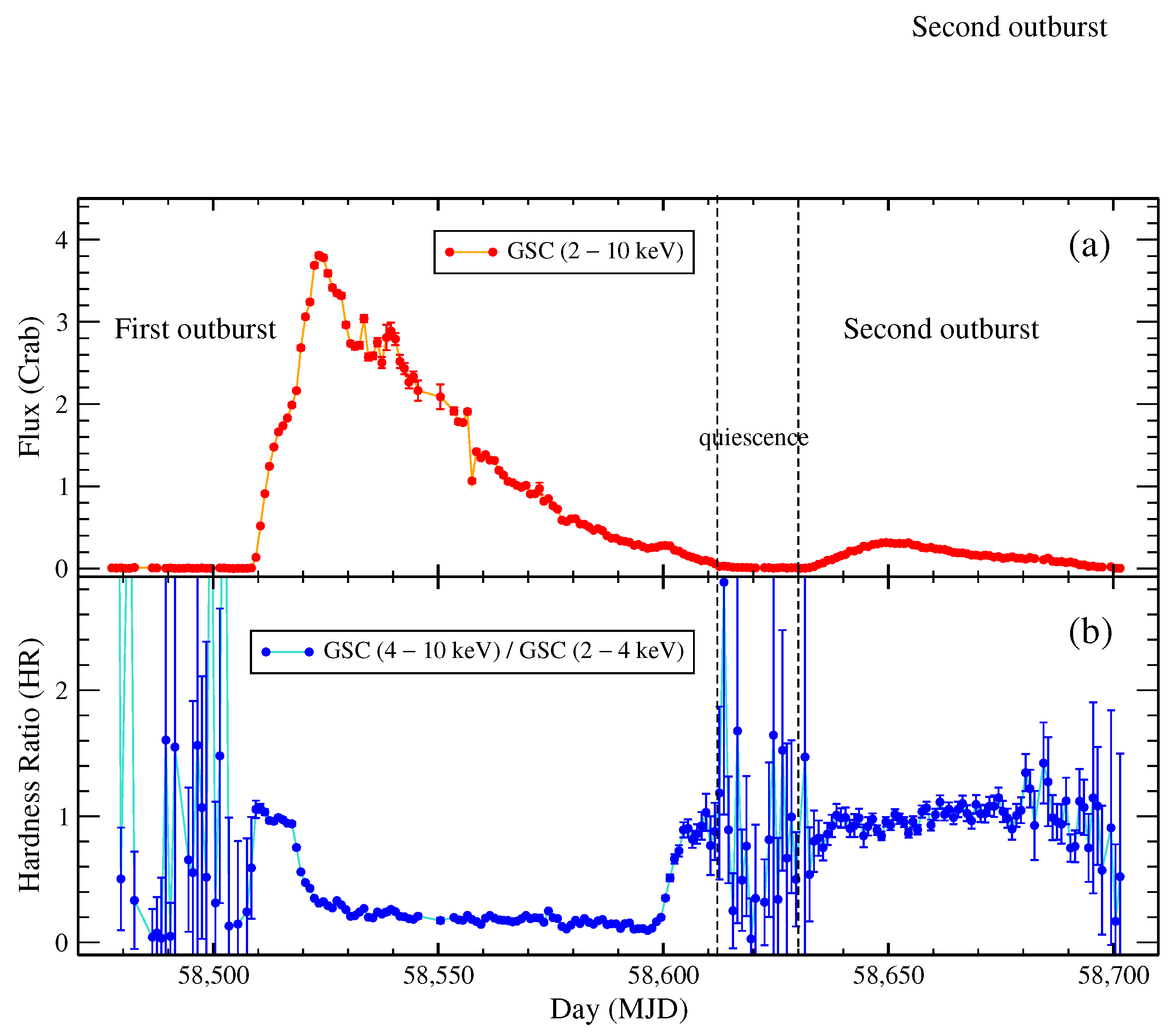
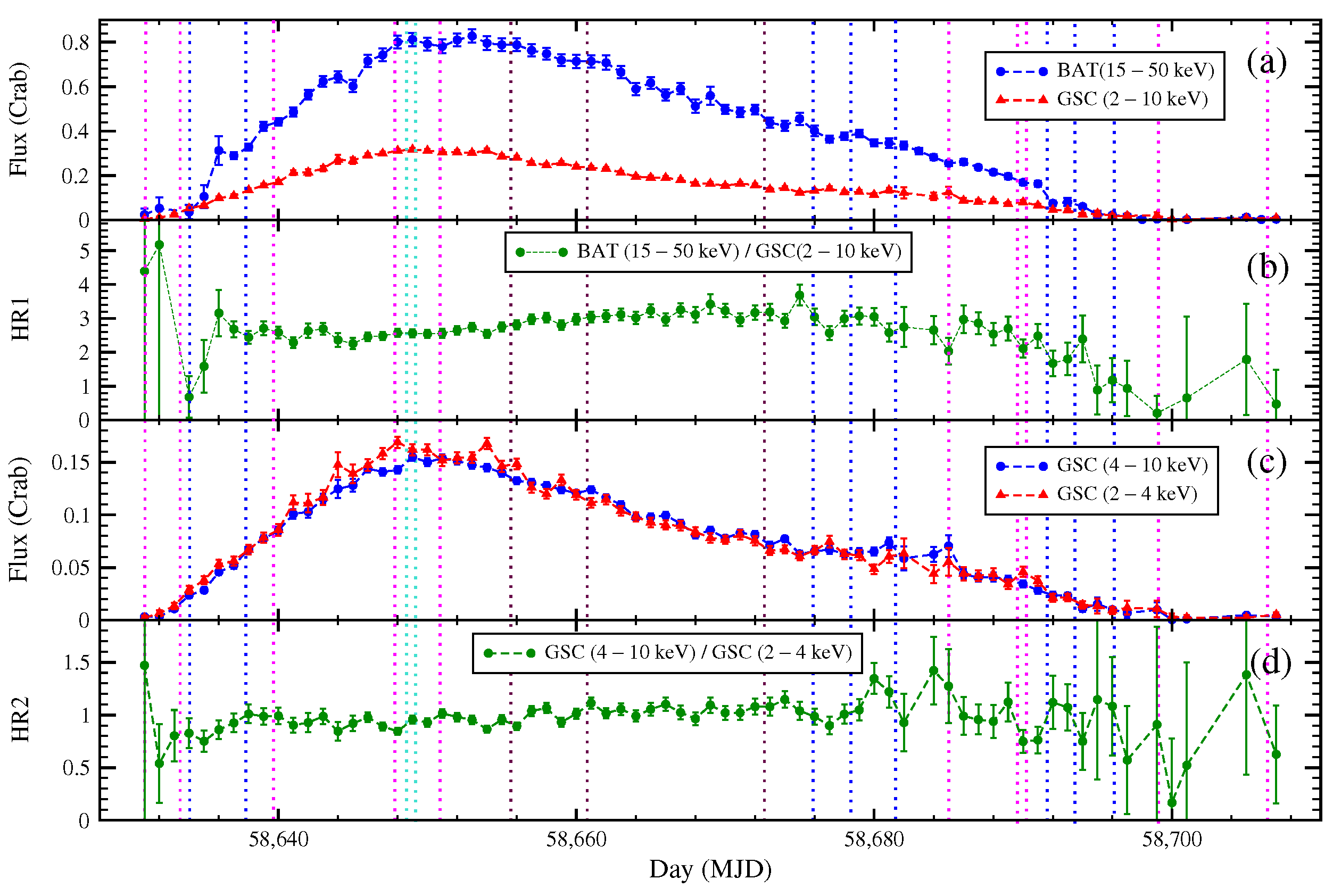
4.1. Temporal Properties

4.1.1. Outburst Profiles

Figure 1 shows the outburst profile, 2–10 keV MAXI/GSC flux (a) and hardness ratio (HR) diagram (b) of BHC MAXI J1348-630 during the first and second outbursts. From the figure, we can see that the source went to quiescence (for ~20 days) after the completion of its first outburst (MJD ~ 58,500 to MJD ~ 58,610) and again rebrightened from MJD ~ 58,630. The second outburst was a mini outburst compared to the first one.

Figure 2 shows the light curves in different energy ranges and the hardness ratios of the second outburst in 2019 of BHC MAXI J1348-630. Panel (a) of Figure 2 shows the variation of 15–50 keV Swift/BAT flux (online blue) and 2–10 keV MAXI/GSC flux (online red). Panel (c) shows the variation of MAXI/GSC flux in two different energy bands: 4–10 keV (online blue) and 2–4 keV (online red). The outburst started on MJD ~ 58,630 (27 May 2019) and returned to quiescence after MJD ~ 58,707 (12 August 2019). According to the variation of flux or count rates in light curve profiles, outbursts are generally divided into two categories: fast-rise slow-decay (FRSD) and slow-rise slow-decay (SRSD) [75]. From light curve profiles, this outburst can be characterized as slow-rise slow-decay (SRSD). As seen in panel (a), both the Swift/BAT flux (15–50 keV) and the total MAXI/GSC flux (2–10 keV) started to increase slowly from MJD ~ 58,630. At MJD ~ 58,650, both the fluxes reached their maximum values, and afterward started to decrease slowly. The fluxes reached quiescence after MJD ~ 58,701. Hard (BAT) flux was dominant over soft (GSC) flux during the entire outburst. Panel (c) shows that flux is low in both energy bands at the start of the outburst. Here, the fluxes gained maximum values near MJD ~ 58,650. Afterwards, both fluxes declined slowly till the end of the outburst.

4.1.2. Hardness Ratio

Hardness ratio (HR) is defined as the ratio of hard X-ray flux to soft X-ray flux. Variation of the HR provides us with a rough idea of the evolution of the flow dynamics of the source, as it is believed that the origin of soft X-ray flux is thermal and hard X-ray flux is non-thermal. The HR is generally high in harder states (HS and HIMS), since high-energy photons dominate over soft photons in harder states. The HR is low in softer states (SIMS and SS) as the reverse condition takes place in softer states. For a complete outburst, the HR remains high at the beginning of the outburst since the BH remains in the hard state (rising). As time progresses the HR gradually decreases in the rising intermediate states (HIMS and SIMS). In the SS, HR has a low value and remains almost constant. The HR gradually increases in the declining intermediate states and becomes roughly constant at a high value in the HS (declining).

In Figure 2, we show two HRs in (HR1 and HR2 in (b) and (d), respectively): (b) shows the ratio of 15–50 keV Swift/BAT flux to 2–10 keV total MAXI/GSC flux, and (d) shows the ratio of 4–10 keV MAXI/GSC hard flux to 2–4 keV MAXI/GSC soft flux. In HR1 (b) we notice that at the beginning of the outburst, the HR has a value of ~2.7 near MJD ~ 58,639. The value slowly increases to 3.42 around MJD ~ 58,669, and after that it slowly decreases till the end of the outburst. In HR2 (d), at the beginning of the outburst, the HR was around ~1, and it stayed there until MJD ~ 58,679. After that, the HR slightly increased to a value of 1.42 at MJD 58,684 and decreased afterwards till the end of the outburst. There, we did not find any signatures of state transition in either of the HRs (HR1 and HR2) as could be seen for a complete or normal outburst of classical BH sources. The HRs varied a little around a certain value throughout the outburst. From the hardness ratio, we can roughly say that the source did not go to softer states; rather, it remained in harder states throughout the outburst. To confirm this, we need to perform spectral analysis.

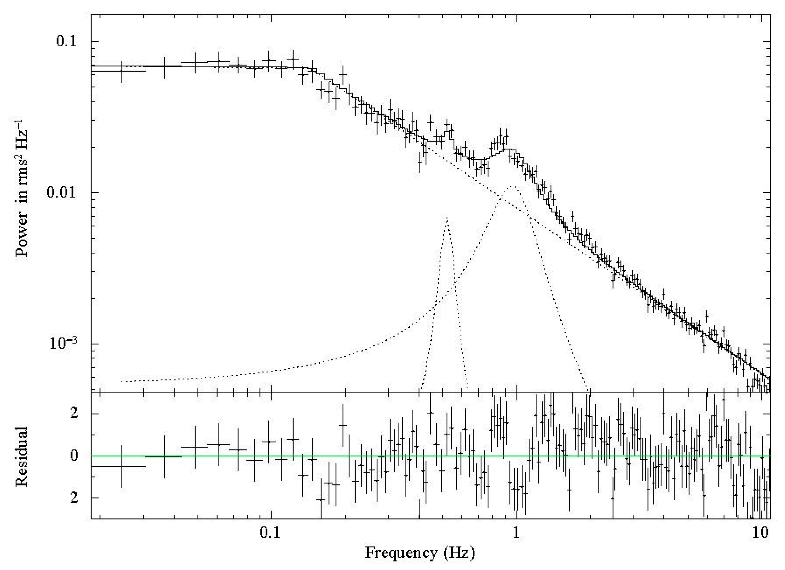
4.1.3. Power Density Spectra

We studied the power-density spectra (PDS) generated with the 0.01 s light curves of AstroSat/LAXPC (3–80 keV) and NICER (1–10 keV). We observed QPOs only on two days, 14 June 2019 and 15 June 2019, in AstroSat/LAXPC data. A QPO of centroid frequency $0.96\pm 0.01$ Hz was observed on 14 June 2019 (MJD = 58,648.6) with a Q-value of $2.23\pm 0.21$ and $6.87\pm 0.4\%$ rms. Figure 3 is a continuum-fitted PDS observed on 14 June 2019. We fitted the PDS with a broken powerlaw and two Lorentzian models. In the PDS, it can be seen that along with the primary QPO at $0.96\pm 0.01$ Hz, there is one more QPO feature at $0.52\pm 0.01$ Hz. The Q-value of this weaker QPO is $8.67\pm 1.45$, and the rms value is $0.80\pm 0.1\%$. This is a sub-harmonic of the primary QPO observed at $0.96\pm 0.01$ Hz. Another QPO was observed on 15 June 2019 (MJD = 58,649.2) with a centroid frequency of $0.95\pm 0.02$ Hz and a Q-value of $2.57\pm 0.42$ and $12.0\pm 1.1\%$ rms. We also calculated the value of the characteristic frequency with the formula ${\nu }_{max}=\sqrt{{\nu }_0^2+{(\Delta /2)}^2}$, where ${\nu }_0$ is the centroid frequency, and $\Delta$ is the FWHM of the Lorentzian [76,77,78]. For 14 June 2019, the value of the characteristic frequency of the primary QPO is $0.98\pm 0.02$ Hz, and on the next day it is observed at $0.98\pm 0.03$ Hz. Note, we did not observe any prominent QPO nature in the NICER data; this might be due to lower effective area and lower energy band compared to AstroSat/LAXPC.

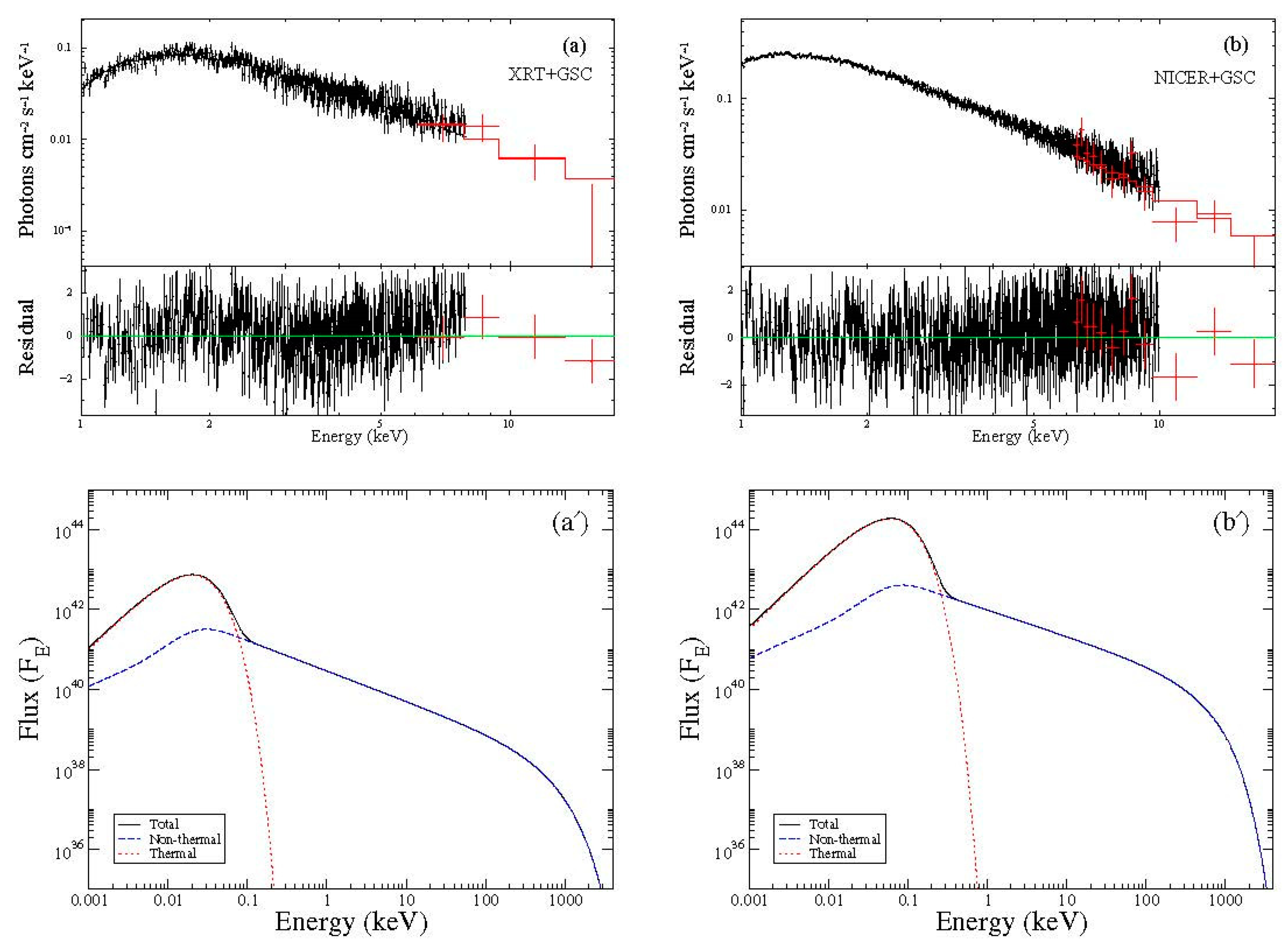
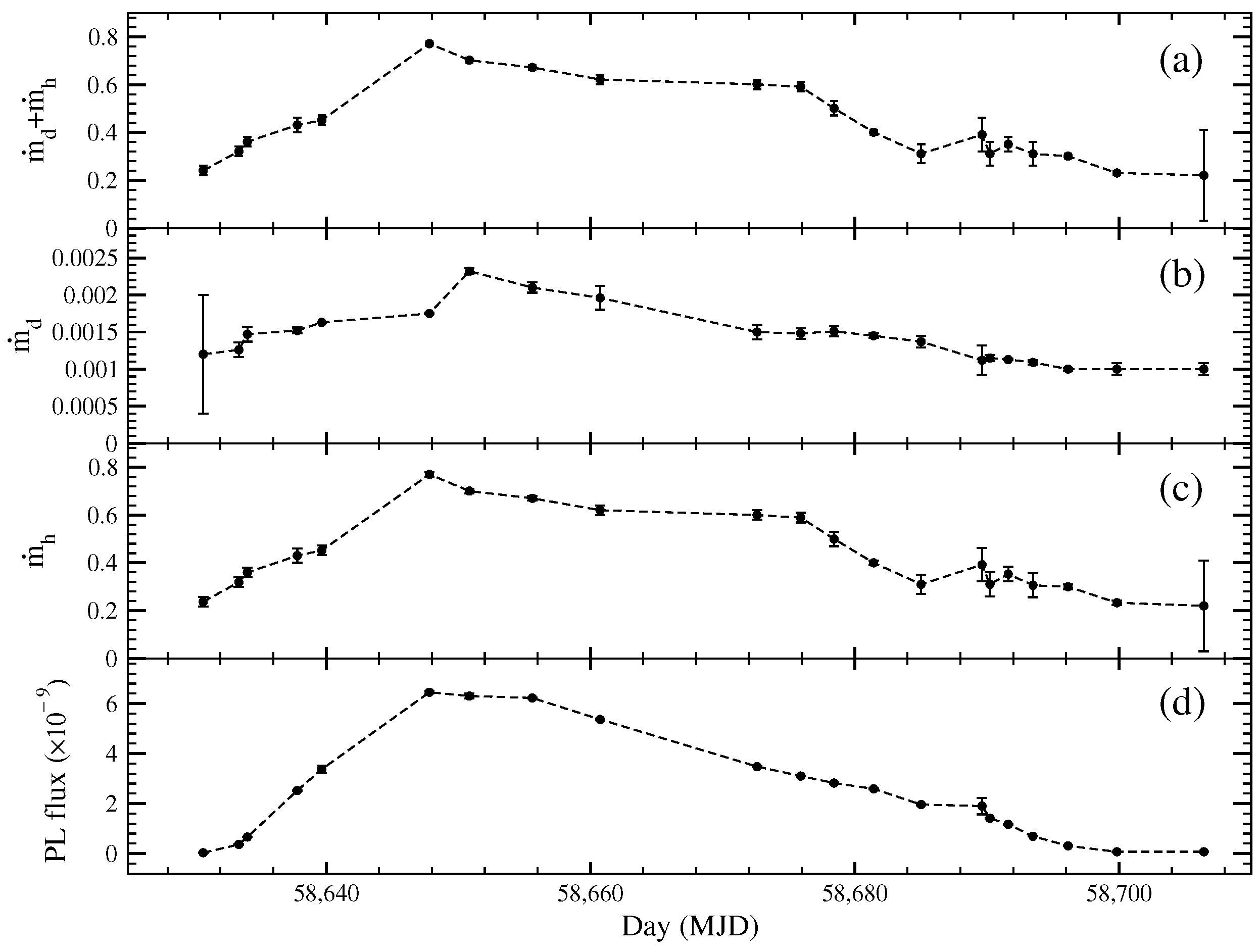
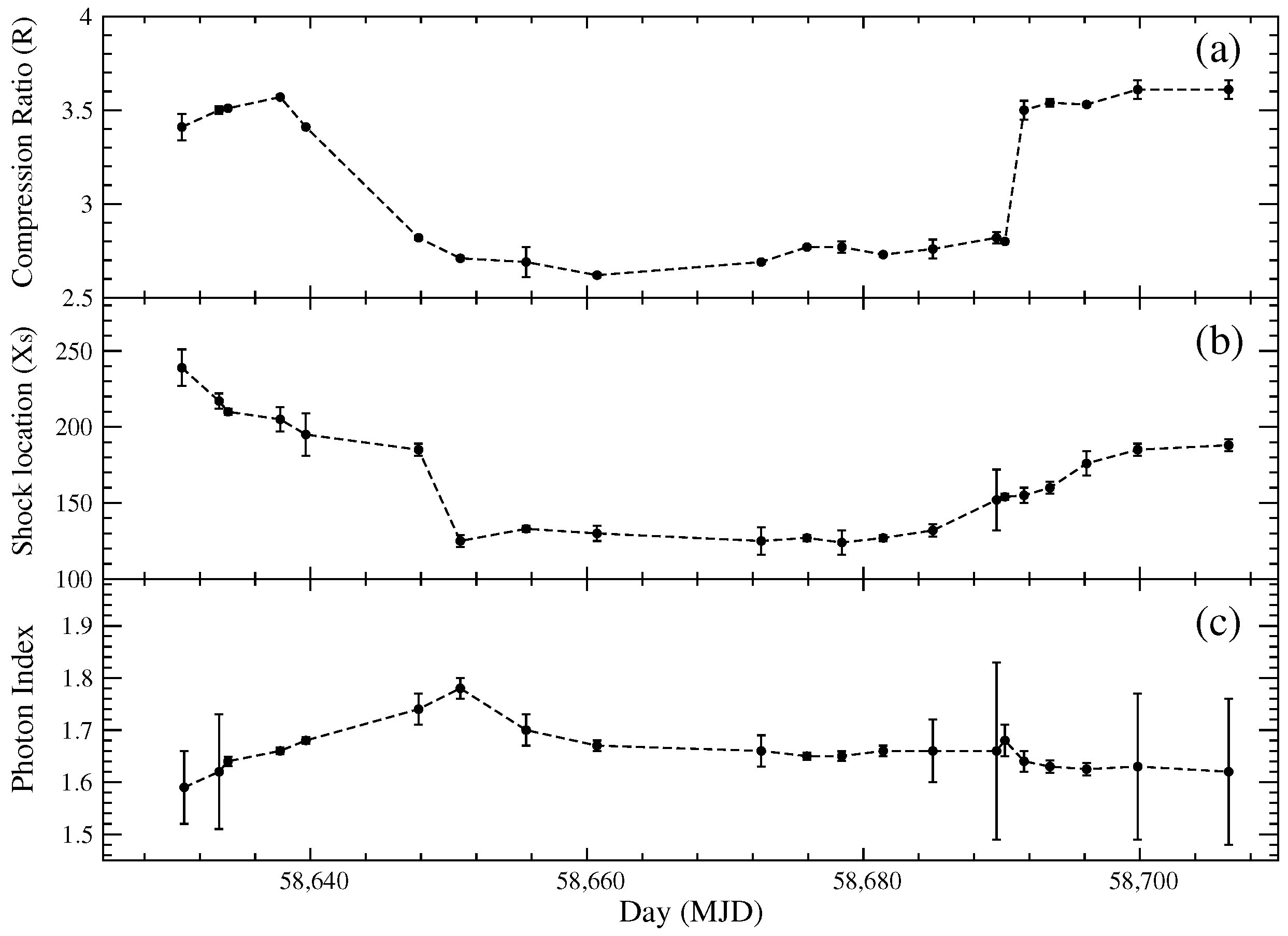
4.2. Spectral Properties

To get an idea about the source and its evolution during the outburst, the study of the spectral properties is very important. As discussed earlier, we used 1–20 keV combined data from Swift/XRT and MAXI/GSC (8 OBSIDs), 1–20 keV NICER and MAXI/GSC (8 OBSIDs), 1–8 keV Swift/XRT (2 OBSIDs) and 4–78 keV NuSTAR data (3 OBSIDs) for the spectral analysis of BHC MAXI J1348-630 during this outburst. First, we fitted all 15 observations of Swift/XRT, (Swift/XRT+MAXI/GSC) data and (NICER+MAXI/GSC) data with the powerlaw (PL) model. The fitted parameters are shown in

Table 2. Model-fitted parameters for Swift/XRT, combined NICER+MAXI/GSC and Swift/XRT+MAXI/GSC spectra (mass, $M_{BH}$, is frozen at 9.1 $M_{\odot }$ for TCAF model).

ID${}^{\left[1\right]}$	${\mathit{n}}_{\mathit{H}}^{\left[2\right]}$	${\mathsf{\Gamma }}^{\left[3\right]}$	${\mathit{f}\mathit{l}\mathit{u}\mathit{x}}^{\left[3\right]}$	${\mathit{\chi }}^2$/dof${}^{\left[5\right]}$	${\dot{\mathit{m}}}_{\mathit{d}}$${}^{\left[4\right]}$	${\dot{\mathit{m}}}_{\mathit{h}}$${}^{\left[4\right]}$	R${}^{\left[4\right]}$	${\mathit{X}}_{\mathit{s}}$${}^{\left[4\right]}$	${\mathit{\chi }}^2$/dof${}^{\left[5\right]}$
(1)	(2)	(3)	(4)	(5)	(6)	(7)	(8)	(9)	(10)
X1	${0.64}^{\pm 0.20}$	${1.59}^{\pm 0.07}$	${0.36}^{\pm 0.04}$	22/27	${1.20}^{\pm 0.08}$	${0.24}^{\pm 0.02}$	${3.41}^{\pm 0.07}$	${239}^{\pm 12}$	19/24
X2	${0.78}^{\pm 0.14}$	${1.62}^{\pm 0.11}$	${3.67}^{\pm 0.25}$	199/197	${1.26}^{\pm 0.10}$	${0.32}^{\pm 0.02}$	${3.50}^{\pm 0.02}$	${217}^{\pm 5}$	197/194
NI1	${0.66}^{\pm 0.05}$	${1.64}^{\pm 0.01}$	${6.64}^{\pm 0.03}$	764/709	${1.50}^{\pm 0.10}$	${0.36}^{\pm 0.02}$	${3.51}^{\pm 0.002}$	${210}^{\pm 2}$	777/706
NI2	${0.51}^{\pm 0.03}$	${1.66}^{\pm 0.01}$	${25.2}^{\pm 0.10}$	924/839	${1.52}^{\pm 0.04}$	${0.43}^{\pm 0.03}$	${3.57}^{\pm 0.008}$	${205}^{\pm 8}$	996/836
X3	${0.65}^{\pm 0.09}$	${1.68}^{\pm 0.06}$	${33.7}^{\pm 1.50}$	721/622	${1.63}^{\pm 0.01}$	${0.45}^{\pm 0.02}$	${3.41}^{\pm 0.01}$	${195}^{\pm 14}$	725/619
X4	${0.62}^{\pm 0.05}$	${1.74}^{\pm 0.03}$	${64.5}^{\pm 0.50}$	959/686	${1.75}^{\pm 0.01}$	${0.77}^{\pm 0.01}$	${2.82}^{\pm 0.01}$	${185}^{\pm 4}$	932/683
X5	${0.50}^{\pm 0.13}$	${1.78}^{\pm 0.02}$	${63.0}^{\pm 1.00}$	707/627	${2.32}^{\pm 0.04}$	${0.70}^{\pm 0.01}$	${2.71}^{\pm 0.01}$	${125}^{\pm 4}$	725/624
NI3	${0.51}^{\pm 0.03}$	${1.65}^{\pm 0.01}$	${31.0}^{\pm 0.10}$	788/779	${1.48}^{\pm 0.07}$	${0.59}^{\pm 0.02}$	${2.77}^{\pm 0.01}$	${127}^{\pm 2}$	816/776
NI4	${0.53}^{\pm 0.02}$	${1.65}^{\pm 0.01}$	${28.2}^{\pm 0.20}$	1037/872	${1.51}^{\pm 0.07}$	${0.50}^{\pm 0.03}$	${2.77}^{\pm 0.03}$	${124}^{\pm 8}$	1099/869
NI5	${0.55}^{\pm 0.03}$	${1.66}^{\pm 0.01}$	${25.9}^{\pm 0.20}$	979/841	${1.45}^{\pm 0.03}$	${0.40}^{\pm 0.01}$	${2.73}^{\pm 0.01}$	${127}^{\pm 2}$	964/838
X6	${0.79}^{\pm 0.20}$	${1.66}^{\pm 0.06}$	${19.6}^{\pm 0.40}$	561/522	${1.37}^{\pm 0.08}$	${0.31}^{\pm 0.04}$	${2.76}^{\pm 0.05}$	${132}^{\pm 4}$	570/519
X7	${0.50}^{\pm 0.29}$	${1.66}^{\pm 0.17}$	${19.0}^{\pm 3.30}$	57/48	${1.12}^{\pm 0.20}$	${0.39}^{\pm 0.07}$	${2.82}^{\pm 0.03}$	${152}^{\pm 20}$	55/45
X8	${0.93}^{\pm 0.25}$	${1.68}^{\pm 0.03}$	${14.1}^{\pm 0.20}$	596/489	${1.15}^{\pm 0.04}$	${0.31}^{\pm 0.05}$	${2.80}^{\pm 0.01}$	${154}^{\pm 2}$	596/486
NI6	${0.61}^{\pm 0.01}$	${1.64}^{\pm 0.02}$	${11.7}^{\pm 0.20}$	771/801	${1.13}^{\pm 0.01}$	${0.35}^{\pm 0.03}$	${3.50}^{\pm 0.05}$	${155}^{\pm 5}$	899/798
NI7	${0.60}^{\pm 0.02}$	${1.63}^{\pm 0.01}$	${6.91}^{\pm 0.03}$	612/637	${1.09}^{\pm 0.03}$	${0.31}^{\pm 0.05}$	${3.54}^{\pm 0.02}$	${160}^{\pm 4}$	639/634
NI8	${0.63}^{\pm 0.04}$	${1.62}^{\pm 0.01}$	${3.11}^{\pm 0.05}$	469/517	${1.00}^{\pm 0.02}$	${0.30}^{\pm 0.01}$	${3.53}^{\pm 0.01}$	${176}^{\pm 8}$	468/514
X9	${0.83}^{\pm 0.13}$	${1.63}^{\pm 0.14}$	${0.71}^{\pm 0.04}$	55/50	${1.00}^{\pm 0.08}$	${0.23}^{\pm 0.01}$	${3.61}^{\pm 0.05}$	${185}^{\pm 4}$	56/47
X10	${0.84}^{\pm 0.04}$	${1.62}^{\pm 0.14}$	${0.72}^{\pm 0.04}$	64/52	${1.00}^{\pm 0.08}$	${0.22}^{\pm 0.19}$	${3.61}^{\pm 0.05}$	${188}^{\pm 4}$	65/49

^[1] ID of the observed dates as mentioned in Table 1 (Col. 1). ^[2] Model-fitted value of hydrogen column density (n_H) in 10²² atoms per cm⁻² (Col. 2). ^[3] PL model-fitted photon index (Γ) in Col. 3. ^[3] PL model-fitted flux in Col. 4 in 10⁻¹⁰ order ^[4] TCAF model-fitted parameters: disk rate (${\dot{m}}_d$ in Eddington rate ${\dot{M}}_{Edd}$) in 10⁻³ order, halo rate (${\dot{m}}_h$ in ${\dot{M}}_{Edd}$) compression ratio (R) and shock location (X_s in Schwarzschild radius r_s); Cols. 6–9, respectively. ^[5] PL and TCAF model-fitted ${\chi }_{red}^2$ values; Cols. 5 and 10, respectively, as ${\chi }^2$/dof, where ‘dof’ represents degrees of freedom. Note: We present average values of 90% confidence ± parameter error values, which are obtained using ‘err’ task in XSPEC.

. Since there were hints of presence of reflection in the NuSTAR spectra (after fitting spectra with only the PL or TCAF model), we fitted the three publicly available NuSTAR data with the REFLECT*powerlaw model along with a Gaussian line. The values of the fitted parameters are shown in

Table 3. Fitted parameters for NuSTAR data with PL/REFLECT*PL model along with a Gaussian line.

	ID${}^{\left[1\right]}$	${\mathit{n}}_{\mathit{H}}$${}^{\left[2\right]}$	${rel}_{refl}$${}^{\left[3\right]}$	$\mathit{c}\mathit{o}\mathit{s}\mathit{I}\mathit{n}\mathit{c}\mathit{l}$${}^{\left[3\right]}$	${\mathsf{\Gamma }}^{\left[4\right]}$	${\mathit{f}\mathit{l}\mathit{u}\mathit{x}}^{\left[4\right]}$	${\mathit{n}\mathit{o}\mathit{r}\mathit{m}}^{\left[4\right]}$	lineE${}^{\left[5\right]}$	${\mathit{\sigma }}^{\left[5\right]}$	norm${}^{\left[5\right]}$	${\mathit{\chi }}^2$/dof${}^{\left[6\right]}$
	(1)	(2)	(3)	(4)	(5)	(6)	(7)	(8)	(9)	(10)	(11)
Model 1:	NU1	${1.01}^{\pm 0.12}$			${1.63}^{\pm 0.01}$	${59.5}^{\pm 0.30}$	${1.46}^{\pm 0.01}$	${6.20}^{\pm 0.19}$	${0.49}^{\pm 0.11}$	$2^{\pm 0.5}$	2494/1500
TBabs*(PL	NU2	${1.04}^{\pm 0.12}$			${1.60}^{\pm 0.01}$	${52.4}^{\pm 0.10}$	${1.17}^{\pm 0.01}$	${6.20}^{\pm 0.17}$	${0.51}^{\pm 0.10}$	$2^{\pm 0.5}$	2689/1501
+Gaussian)	NU3	${1.01}^{\pm 0.13}$			${1.58}^{\pm 0.01}$	${34.3}^{\pm 0.20}$	${0.74}^{\pm 0.01}$	${6.46}^{\pm 0.05}$	${0.22}^{\pm 0.01}$	$1^{\pm 0.1}$	2248/1439
Model 2:	NU1	${0.74}^{\pm 0.14}$	${0.23}^{\pm 0.05}$	${0.86}^{\pm 0.15}$	${1.70}^{\pm 0.01}$	${62.2}^{\pm 0.20}$	${1.55}^{\pm 0.03}$	${6.40}^{\pm 0.07}$	${0.75}^{\pm 0.08}$	$4^{\pm 0.6}$	1594/1498
TBabs*(reflect	NU2	${0.50}^{\pm 0.26}$	${0.26}^{\pm 0.05}$	${0.70}^{\pm 0.14}$	${1.67}^{\pm 0.01}$	${53.6}^{\pm 0.30}$	${1.28}^{\pm 0.02}$	${6.31}^{\pm 0.08}$	${0.65}^{\pm 0.08}$	$3^{\pm 0.5}$	1553/1499
PL+Gaussian)	NU3	${0.74}^{\pm 0.14}$	${0.26}^{\pm 0.06}$	${0.70}^{\pm 0.17}$	${1.66}^{\pm 0.01}$	${34.8}^{\pm 0.20}$	${0.84}^{\pm 0.01}$	${6.51}^{\pm 0.05}$	${0.25}^{\pm 0.06}$	$1^{\pm 0.2}$	1464/1437

^[1] ID of the observed dates as described in Table 1 (Col. 1). ^[2] Model-fitted value of hydrogen column density n_H in 10²² atoms per cm⁻² (Col. 2). ^[3] In case of reflect model, reflection scaling factor (${rel}_{refl}$) and cosine of inclination angle (cosIncl) are mentioned in Cols. (3–4), respectively. ^[4] In case of PL model, photon index (Γ), flux and norm are mentioned in Cols. 5, 6 and 7, respectively. ^[5] Line energy of the Gaussian line energy (lineE) in keV, line width (sigma) in keV and total photons/cm²/s in the line (norm) in 10⁻³ order; Cols. 8–10, respectively. ^[6] Model-fitted ${\chi }_{red}^2$; Col. 11 as ${\chi }^2$/dof, where ‘dof’ represents degrees of freedom.

.

The PL model gives us a rough idea about the spectral states. To know about the variation of the accretion flow parameters during the outburst, we fitted all the observations with the TCAF model also. Initially, we fitted the spectra with the TCAF model keeping the BH mass ($M_{BH}$) free. From each spectral fit, we obtained the best-fitted value of $M_{BH}$. The $M_{BH}$ values varied between 7.9 $M_{\odot }$ and 10.3 $M_{\odot }$. We averaged these best-fitted mass values to get 9.1 $M_{\odot }$. Then, we kept $M_{BH}$ frozen at this value and refitted all the spectra to obtain the final result. The preliminary values of the fitted parameters of the 1–20 keV XRT+GSC data, 1–8 keV XRT data and the 1–20 keV NICER+GSC spectra are mentioned in

Table A1. Model-fitted parameters for Swift/XRT, combined NICER+MAXI/GSC and Swift/XRT+MAXI/GSC spectra (taking mass ($M_{BH}$) as a free parameter for TCAF model).

ID${}^{\left[1\right]}$	${\mathit{n}}_{\mathit{H}}^{\left[2\right]}$	${\mathsf{\Gamma }}^{\left[3\right]}$	${\mathit{flux}}^{\left[3\right]}$	${\mathit{\chi }}^2$/dof${}^{\left[5\right]}$	${\dot{\mathit{m}}}_{\mathit{d}}$${}^{\left[4\right]}$	${\dot{\mathit{m}}}_{\mathit{h}}$${}^{\left[4\right]}$	R${}^{\left[4\right]}$	${\mathit{X}}_{\mathit{s}}$${}^{\left[4\right]}$	${\mathit{M}}_{\mathbf{BH}}$${}^{\left[4\right]}$	${\mathit{\chi }}^2$/dof${}^{\left[5\right]}$
(1)	(2)	(3)	(4)	(5)	(6)	(7)	(8)	(9)	(10)	(11)
X1	${0.64}^{\pm 0.20}$	${1.59}^{\pm 0.07}$	${0.36}^{\pm 0.04}$	22/27	${1.20}^{\pm 0.08}$	${0.24}^{\pm 0.19}$	${3.41}^{\pm 0.04}$	${239}^{\pm 14}$	${10.1}^{\pm 0.53}$	19/23
X2	${0.78}^{\pm 0.14}$	${1.62}^{\pm 0.11}$	${3.67}^{\pm 0.25}$	199/197	${1.31}^{\pm 0.10}$	${0.32}^{\pm 0.02}$	${3.50}^{\pm 0.02}$	${219}^{\pm 5}$	${7.9}^{\pm 0.21}$	197/193
NI1	${0.66}^{\pm 0.05}$	${1.64}^{\pm 0.01}$	${6.64}^{\pm 0.03}$	764/709	${1.37}^{\pm 0.03}$	${0.34}^{\pm 0.02}$	${3.60}^{\pm 0.002}$	${210}^{\pm 1}$	${7.9}^{\pm 0.05}$	776/705
NI2	${0.51}^{\pm 0.03}$	${1.66}^{\pm 0.01}$	${25.2}^{\pm 0.10}$	924/839	${1.50}^{\pm 0.04}$	${0.38}^{\pm 0.02}$	${3.57}^{\pm 0.003}$	${205}^{\pm 2}$	${7.9}^{\pm 0.03}$	1011/835
X3	${0.65}^{\pm 0.09}$	${1.68}^{\pm 0.06}$	${33.7}^{\pm 1.50}$	721/622	${1.63}^{\pm 0.30}$	${0.45}^{\pm 0.03}$	${3.41}^{\pm 0.01}$	${195}^{\pm 13}$	${8.1}^{\pm 0.08}$	724/618
X4	${0.63}^{\pm 0.06}$	${1.74}^{\pm 0.03}$	${64.5}^{\pm 0.50}$	959/686	${1.79}^{\pm 0.08}$	${0.78}^{\pm 0.01}$	${2.80}^{\pm 0.06}$	${180}^{\pm 14}$	${10.3}^{\pm 0.08}$	931/682
X5	${0.53}^{\pm 0.13}$	${1.78}^{\pm 0.02}$	${63.0}^{\pm 1.00}$	707/627	${2.32}^{\pm 0.04}$	${0.67}^{\pm 0.05}$	${2.70}^{\pm 0.04}$	${125}^{\pm 1}$	${10.2}^{\pm 0.16}$	723/623
NI3	${0.51}^{\pm 0.02}$	${1.65}^{\pm 0.01}$	${31.0}^{\pm 0.10}$	788/779	${1.48}^{\pm 0.07}$	${0.59}^{\pm 0.03}$	${2.77}^{\pm 0.01}$	${127}^{\pm 2}$	${8.0}^{\pm 0.02}$	811/775
NI4	${0.52}^{\pm 0.02}$	${1.65}^{\pm 0.01}$	${28.2}^{\pm 0.20}$	1037/872	${1.50}^{\pm 0.07}$	${0.50}^{\pm 0.03}$	${2.77}^{\pm 0.03}$	${124}^{\pm 7}$	${8.5}^{\pm 0.02}$	1046/868
NI5	${0.55}^{\pm 0.03}$	${1.66}^{\pm 0.01}$	${25.9}^{\pm 0.20}$	979/841	${1.45}^{\pm 0.04}$	${0.40}^{\pm 0.01}$	${2.73}^{\pm 0.01}$	${127}^{\pm 1}$	${7.9}^{\pm 0.03}$	964/837
X6	${0.79}^{\pm 0.20}$	${1.66}^{\pm 0.06}$	${19.6}^{\pm 0.40}$	561/522	${1.39}^{\pm 0.02}$	${0.31}^{\pm 0.04}$	${2.76}^{\pm 0.01}$	${132}^{\pm 1}$	${7.9}^{\pm 0.11}$	569/518
X7	${0.50}^{\pm 0.29}$	${1.66}^{\pm 0.17}$	${19.0}^{\pm 3.30}$	57/48	${1.12}^{\pm 0.20}$	${0.39}^{\pm 0.07}$	${2.82}^{\pm 0.03}$	${152}^{\pm 21}$	${10.2}^{\pm 0.87}$	54/44
X8	${0.93}^{\pm 0.25}$	${1.68}^{\pm 0.03}$	${14.1}^{\pm 0.20}$	596/489	${1.15}^{\pm 0.04}$	${0.30}^{\pm 0.07}$	${2.80}^{\pm 0.01}$	${153}^{\pm 12}$	${7.9}^{\pm 0.07}$	596/485
NI6	${0.61}^{\pm 0.01}$	${1.64}^{\pm 0.02}$	${11.7}^{\pm 0.20}$	771/801	${1.13}^{\pm 0.01}$	${0.35}^{\pm 0.09}$	${3.50}^{\pm 0.01}$	${155}^{\pm 18}$	${8.0}^{\pm 0.02}$	894/797
NI7	${0.60}^{\pm 0.02}$	${1.63}^{\pm 0.01}$	${6.91}^{\pm 0.03}$	612/637	${1.09}^{\pm 0.40}$	${0.31}^{\pm 0.01}$	${3.54}^{\pm 0.02}$	${160}^{\pm 19}$	${9.4}^{\pm 0.03}$	639/633
NI8	${0.63}^{\pm 0.04}$	${1.62}^{\pm 0.01}$	${3.11}^{\pm 0.05}$	469/517	${1.00}^{\pm 0.03}$	${0.30}^{\pm 0.01}$	${3.53}^{\pm 0.17}$	${176}^{\pm 6}$	${8.2}^{\pm 0.05}$	468/513
X9	${0.83}^{\pm 0.13}$	${1.63}^{\pm 0.14}$	${0.71}^{\pm 0.04}$	55/50	${1.00}^{\pm 0.09}$	${0.23}^{\pm 0.01}$	${3.60}^{\pm 0.05}$	${187}^{\pm 3}$	${8.1}^{\pm 0.33}$	56/46
X10	${0.84}^{\pm 0.04}$	${1.62}^{\pm 0.14}$	${0.72}^{\pm 0.04}$	64/52	${1.00}^{\pm 0.08}$	${0.22}^{\pm 0.19}$	${3.61}^{\pm 0.05}$	${188}^{\pm 4}$	${7.9}^{\pm 0.44}$	64/48

^[1] ID of the observed dates as mentioned in Table 1 (Col. 1). ^[2] Model-fitted value of hydrogen column density (n_H) in 10²² atoms per cm⁻² (Col. 2). ^[3] PL model-fitted photon index (Γ); Col. 3. ^[3] PL model-fitted flux; Col. 4 in 10⁻¹⁰ order ^[4] TCAF model-fitted parameters: disk rate (${\dot{m}}_d$ in Eddington rate ${\dot{M}}_{Edd}$) in 10⁻³ order, halo rate (${\dot{m}}_h$ in ${\dot{M}}_{Edd}$) , compression ratio (R), shock location (X_s in Schwarzschild radius r_s) and mass of the black hole (M_BH in solar mass $M_{\odot }$); Cols. 6–10, respectively. ^[5] PL and TCAF model-fitted ${\chi }_{red}^2$ values; Cols. 5 and 11, respectively, as ${\chi }^2$/dof, where ‘dof’ represents degrees of freedom. Note: We present average values of 90% confidence ± parameter error values, which are obtained using ‘err’ task in XSPEC.

. The final results are shown in Table 2. The NuSTAR data is fitted with the TCAF model along with REFLECT model (to account for the reflection) and a Gaussian line to incorporate the Fe K$\alpha$ emission line. The preliminary values of the fitted parameters are shown in

Table A2. Fitted parameters for NuSTAR data with TCAF/REFLECT*TCAF model along with a Gaussian line (taking mass ($M_{BH}$) as a free parameter).

	ID${}^{\left[1\right]}$	${\mathit{n}}_{\mathit{H}}$${}^{\left[2\right]}$	${\mathit{rel}}_{\mathit{refl}}$${}^{\left[3\right]}$	$\mathit{cosIncl}$${}^{\left[3\right]}$	${\dot{\mathit{m}}}_{\mathit{d}}$${}^{\left[4\right]}$	${\dot{\mathit{m}}}_{\mathit{h}}$${}^{\left[4\right]}$	R${}^{\left[4\right]}$	${\mathit{X}}_{\mathit{s}}$${}^{\left[4\right]}$	${\mathit{M}}_{\mathbf{BH}}$${}^{\left[4\right]}$	lineE${}^{\left[5\right]}$	sigma${}^{\left[5\right]}$	norm${}^{\left[5\right]}$	${\mathit{\chi }}^2$/dof${}^{\left[6\right]}$
	(1)	(2)	(3)	(4)	(5)	(6)	(7)	(8)	(9)	(10)	(11)	(12)	(13)
Model 1:	NU1	${0.50}^{\pm 0.12}$			${1.48}^{\pm 0.03}$	${0.61}^{\pm 0.02}$	${3.46}^{\pm 0.13}$	${134}^{\pm 1}$	${7.9}^{\pm 0.03}$	${6.20}^{\pm 0.19}$	${0.80}^{\pm 0.15}$	$4^{\pm 0.8}$	2121/1496
TBabs*(TCAF+	NU2	${0.50}^{\pm 0.12}$			${1.50}^{\pm 0.08}$	${0.60}^{\pm 0.02}$	${3.65}^{\pm 0.12}$	${134}^{\pm 1}$	${10.2}^{\pm 0.08}$	${6.20}^{\pm 0.21}$	${0.79}^{\pm 0.11}$	$6^{\pm 0.7}$	2079/1497
Gaussian)	NU3	${0.50}^{\pm 0.13}$			${1.04}^{\pm 0.04}$	${0.60}^{\pm 0.01}$	${3.42}^{\pm 0.15}$	${134}^{\pm 1}$	${8.4}^{\pm 0.30}$	${6.20}^{\pm 0.24}$	${0.70}^{\pm 0.10}$	$3^{\pm 0.9}$	1767/1435
Model 2:	NU1	${0.50}^{\pm 0.23}$	${0.29}^{\pm 0.03}$	${0.86}^{\pm 0.20}$	${2.10}^{\pm 0.03}$	${0.67}^{\pm 0.01}$	${2.70}^{\pm 0.08}$	${132}^{\pm 1}$	${7.9}^{\pm 0.02}$	${6.30}^{\pm 0.17}$	${0.80}^{\pm 0.24}$	$5^{\pm 0.2}$	1607/1494
TBabs*(reflect*	NU2	${0.50}^{\pm 0.43}$	${0.32}^{\pm 0.12}$	${0.72}^{\pm 0.14}$	${2.00}^{\pm 0.03}$	${0.63}^{\pm 0.02}$	${2.65}^{\pm 0.11}$	${125}^{\pm 3}$	${7.9}^{\pm 0.21}$	${6.31}^{\pm 0.18}$	${0.71}^{\pm 0.24}$	$3^{\pm 0.9}$	1647/1495
TCAF+Gaussian)	NU3	${0.83}^{\pm 0.21}$	${0.32}^{\pm 0.05}$	${0.70}^{\pm 0.17}$	${1.50}^{\pm 0.03}$	${0.60}^{\pm 0.02}$	${2.69}^{\pm 0.12}$	${125}^{\pm 2}$	${10.1}^{\pm 0.25}$	${6.51}^{\pm 0.14}$	${0.21}^{\pm 0.18}$	$1^{\pm 0.1}$	1694/1433

^[1] ID of the observed dates as described in Table 1 (Col. 1). ^[2] Model-fitted value of hydrogen column density n_H in 10²² atoms per cm⁻² (Col. 2). ^[3] For REFLECT*TCAF+Gaussian model, the value of reflection scaling factor (${rel}_{refl}$) and the cosine of inclination angle (cosIncl); Col. 3 and Col. 4, respectively. ^[4] TCAF model-fitted parameters: disk rate (${\dot{m}}_d$ in Eddington rate ${\dot{M}}_{Edd}$) in 10⁻³ order, halo rate (${\dot{m}}_h$ in ${\dot{M}}_{Edd}$), compression ratio (R), shock location (X_s in Schwarzschild radius r_s) and mass of the black hole (M_BH in solar mass $M_{\odot }$); Cols. 5–9, respectively. ^[5] Line energy of the Gaussian line energy (lineE) in keV, line width (sigma) in keV and total photons/cm²/s in the line (norm) in 10⁻³ order; Cols. 10, 11, and 12, respectively. ^[6] Model-fitted ${\chi }_{red}^2$; Col. 13 as ${\chi }^2$/dof, where ‘dof’ represents degrees of freedom.

(where we kept the $M_{BH}$ as a free parameter). The final fitted parameters are mentioned in

Table 4. Fitted parameters for NuSTAR data with TCAF/REFLECT*TCAF model along with a Gaussian line (mass, $M_{BH}$, is frozen at 9.1 $M_{\odot }$ for TCAF model).

	ID${}^{\left[1\right]}$	${\mathit{n}}_{\mathit{H}}$${}^{\left[2\right]}$	${\mathit{rel}}_{\mathit{refl}}$${}^{\left[3\right]}$	$\mathit{cosIncl}$${}^{\left[3\right]}$	${\dot{\mathit{m}}}_{\mathit{d}}$${}^{\left[4\right]}$	${\dot{\mathit{m}}}_{\mathit{h}}$${}^{\left[4\right]}$	R${}^{\left[4\right]}$	${\mathit{X}}_{\mathit{s}}$${}^{\left[4\right]}$	lineE${}^{\left[5\right]}$	sigma${}^{\left[5\right]}$	norm${}^{\left[5\right]}$	${\mathit{\chi }}^2$/dof${}^{\left[6\right]}$
	(1)	(2)	(3)	(4)	(5)	(6)	(7)	(8)	(9)	(10)	(11)	(12)
Model 1:	NU1	${0.50}^{\pm 0.12}$			${1.48}^{\pm 0.02}$	${0.61}^{\pm 0.02}$	${3.44}^{\pm 0.10}$	${134}^{\pm 1}$	${6.20}^{\pm 0.20}$	${0.80}^{\pm 0.16}$	$4^{\pm 0.8}$	2113/1497
TBabs*(TCAF+	NU2	${0.50}^{\pm 0.12}$			${1.50}^{\pm 0.10}$	${0.60}^{\pm 0.04}$	${3.65}^{\pm 0.11}$	${134}^{\pm 1}$	${6.20}^{\pm 0.21}$	${0.76}^{\pm 0.08}$	$6^{\pm 0.7}$	1995/1498
Gaussian)	NU3	${0.50}^{\pm 0.13}$			${1.04}^{\pm 0.03}$	${0.60}^{\pm 0.03}$	${3.43}^{\pm 0.12}$	${134}^{\pm 1}$	${6.20}^{\pm 0.24}$	${0.73}^{\pm 0.10}$	$3^{\pm 0.9}$	1791/1436
Model 2:	NU1	${0.50}^{\pm 0.23}$	${0.29}^{\pm 0.05}$	${0.86}^{\pm 0.20}$	${2.10}^{\pm 0.07}$	${0.67}^{\pm 0.01}$	${2.70}^{\pm 0.08}$	${133}^{\pm 2}$	${6.33}^{\pm 0.17}$	${0.80}^{\pm 0.25}$	$5^{\pm 0.2}$	1621/1495
TBabs*(reflect*	NU2	${0.50}^{\pm 0.43}$	${0.32}^{\pm 0.13}$	${0.74}^{\pm 0.21}$	${2.00}^{\pm 0.16}$	${0.62}^{\pm 0.02}$	${2.62}^{\pm 0.01}$	${130}^{\pm 5}$	${6.33}^{\pm 0.18}$	${0.69}^{\pm 0.19}$	$3^{\pm 0.9}$	1670/1496
TCAF+Gaussian)	NU3	${0.80}^{\pm 0.21}$	${0.33}^{\pm 0.06}$	${0.72}^{\pm 0.17}$	${1.50}^{\pm 0.10}$	${0.60}^{\pm 0.02}$	${2.69}^{\pm 0.01}$	${125}^{\pm 9}$	${6.51}^{\pm 0.05}$	${0.22}^{\pm 0.07}$	$1^{\pm 0.2}$	1684/1434

^[1] IDs of the observed dates as described in Table 1 (Col. 1). ^[2] Model-fitted value of hydrogen column density n_H in 10²² atoms per cm⁻² (Col. 2). ^[3] In case of REFLECT*TCAF+Gaussian model, the value of reflection scaling factor (${rel}_{refl}$) and the cosine of inclination angle (cosIncl); Col. 3 and Col. 4, respectively. ^[4] TCAF model-fitted parameters: disk rate (${\dot{m}}_d$ in Eddington rate ${\dot{M}}_{Edd}$) in 10⁻³ order, halo rate (${\dot{m}}_h$ in ${\dot{M}}_{Edd}$), compression ratio (R) and shock location (X_s in Schwarzschild radius r_s); Cols. 5–8. ^[5] Line energy of the Gaussian line energy (lineE) in keV, line width (sigma) in keV and total photons/cm²/s in the line (norm) in 10⁻³ order; Cols. 9, 10 and 11, respectively. ^[6] Model-fitted ${\chi }_{red}^2$; Col. 12 as ${\chi }^2$/dof, where ‘dof’ represents degrees of freedom.

(where we froze the $M_{BH}$ at 9.1 $M_{\odot }$).

Figure 4a,b show TCAF model-fitted spectra using different spectral data. The left panel shows the TCAF model-fitted combined spectrum of Swift/XRT (OBSID 00011107047) with MAXI/GSC in 1–20 keV energy band during MJD = 58,690.23, and the right panel shows the TCAF model-fitted spectrum of the combined NICER (OBSID 2200530170) and simultaneous MAXI/GSC during MJD = 58,675.9 in 1–20 keV enery band. The bottom panels of Figure 4 (${\mathrm{a}}^{\prime }$,${\mathrm{b}}^{\prime }$ show two theoretical model unabsorbed raw spectra, which were used to fit observed spectra in the top panels. We can see the thermal and non-thermal components of the theoretical spectra separately in the plots. The thermal part originates from the pre-shock flow via bremsstrahlung and Comptonization processes, while the non-thermal part of the spectra originates from the emitted photons from the hot Compton cloud or CENBOL via inverse Comptonization of the intercepted thermal photons (see [26,32] and references therein).

Figure 5 shows the fitted spectrum of the NuSTAR data (OBSID 80502304002) with different models. Panel (a) shows the PL+Gaussian model-fitted spectrum, which shows a signature of the reflection component in the disk ~10 keV. Thus, we refitted the spectrum with REFLECT*powerlaw+Gaussian model (panel (b)). The model-fitted reduced ${\chi }^2$ is improved from 1.66 to 1.06. This signifies the spectrum is fitted better with the REFLECT*powerlaw+Gaussian model. Panels (c) and (d) show the fitted spectrum of that particular observation with TCAF+Gaussian model and REFLECT*TCAF+Gaussian model. In the last set, continuum due to primary emission is fitted with TCAF and REFLECT, where REFLECT is used to fit the reflection part (due to reprocessed photons) of the spectrum. It is clear from the figure that the spectrum is fitted better when we added the REFLECT model with the TCAF model to account for the reflection. The reduced ${\chi }^2$ value decreased from 1.41 to 1.08.

Figure 6a shows the unabsorbed model components of the fitted spectrum shown in Figure 5d for the NuSTAR OBSID 80502304002 (MJD = 58,655.60) from XSPEC. Here, the contribution of the TCAF model, REFLECT model and the Gaussian line are shown separately. The theoretical TCAF model-generated unabsorbed raw spectrum with its two components (thermal and non-thermal) is shown in panel (b) of Figure 6.

Figure 7 and Figure 8 show variation of the different model-fitted parameters. In Figure 7, we show the evolution of (a) the TCAF model-fitted total accretion rate (${\dot{m}}_d$ + ${\dot{m}}_h$), (b) the Keplerian disk rate (${\dot{m}}_d$) and (c) the sub-Keplerian halo rate (${\dot{m}}_h$). Both the rates (disk rate and halo rate) are in units of Eddington rate (${\dot{M}}_{Edd}$). Panel (d) of Figure 7 shows the variation of powerlaw flux. In Figure 8, we show the variation of the TCAF model-fitted (a) shock compression ratio (R) and (b) the shock location ($X_s$) in ($r_s$). Panel (c) of Figure 8 shows the variation of the photon index.

The photon index of powerlaw ($\mathsf{\Gamma }$) varied from 1.59–1.78 (Figure 8c). On the first day of observation, the value of $\mathsf{\Gamma }$ was 1.59. Then, it gradually increased to a maximum value of 1.78 on MJD ~ 58,650. After that, $\mathsf{\Gamma }$ started to decrease; it attained a minimum value of 1.63 on MJD ~ 58,693 and remained there till the end of the outburst.

At the start of the outburst, the halo accretion rate (${\dot{m}}_h$) was ~0.237 ${\dot{M}}_{Edd}$ (Figure 7c). As the outburst continued, the ${\dot{m}}_h$ gradually increased and reached its maximum on MJD ~ 58,648. After that, the halo rate started to decrease and attained its minimum on MJD ~ 58,685. The ${\dot{m}}_h$ again increased briefly after MJD ~ 58,685, and shortly after MJD ~ 58,692, it declined again till the end of the outburst. At the start of the outburst, the disk rate (${\dot{m}}_d$) was 0.0012 ${\dot{M}}_{Edd}$ (very small compared to the halo rate). The disk rate gradually increased and attained its maximum on MJD ~ 58,651 (3 days after the peak of the halo rate). Thereafter, the disk rate started to decrease and attained the minimum value on MJD ~ 58,696 and remained at this value till the end of the observed period. Since the value of the disk rate was very small compared to the halo rate, the nature of the variation of total accretion rate (${\dot{m}}_d$ + ${\dot{m}}_h$) is same as the halo rate. The powerlaw continuum and its high-energy cutoff powerlaw models signify the non-thermal inverse-Comptonized high energy part of the spectra, whereas the ${\dot{m}}_h$ parameter of TCAF measures the rate of accretion of sub-Keplerian mass, which is responsible for forming the corona and inverse-Comptonization cloud. There is bound to be some correlation between ${\dot{m}}_h$ and powerlaw flux. Indeed, as can be seen from Figure 7d, the powerlaw flux and the ${\dot{m}}_h$ shows similar variation during the course of the outburst. When ${\dot{m}}_h$ becomes high, it signifies the presence of large amounts of sub-Keplerian matter, which emits a large amount of inverse-Comptonized high-energy X-rays, which in turn increases the flux of the powerlaw part of the spectrum. When ${\dot{m}}_h$ becomes low, the opposite phenomena happens, and powerlaw flux also reduces.

In Figure 8, it can be noticed that the shock compression ratio (R) is high, and the shock location ($X_s$) is far away from the BH at the start of the outburst ((a) and (b)). On the first day (MJD ~ 58,630) of the outburst, the shock ($X_s$) was located at a distance of ~240 $r_s$. The $X_s$ started to decrease slowly with time and attained its minimum of ~125 $r_s$ on MJD ~ 58,651. It remained between 125 $r_s$–132 $r_s$ till MJD ~ 58,685, and after that, it started to increase gradually. On the last day of the outburst (MJD = 58,706), the shock moved away at a distance of 188 $r_s$. The variation of the shock compression ratio (R), i.e., the ratio of post shock to pre-shock matter density, is shown in Figure 8a. The value of R varied from 2.7 to 3.61. Initially, the value of R was around ~3.5 at the start of the outburst. After that, it decreased to a value 2.8 at MJD ~ 58,647. The value of R varied from 2.7–2.8 up to MJD ~ 58,690, and afterwards it started to increase. R reached 3.61 on the last day of our observation.

The spectral results depict the absence of the softer states during the outburst. The photon index ($\mathsf{\Gamma }$) never exceeded 1.8. Throughout the outburst, the halo rate (${\dot{m}}_h$) was dominant over the disk rate (${\dot{m}}_d$). Although the shock location moved slightly closer to the BH during the middle phase of the outburst, $X_s$ was never smaller than 125 $r_s$. The minimum value of the compression ratio was 2.7 during the outburst. From these results, we can conclude that BHC MAXI J1348-630 went through the hard state (HS) only during the second outburst of 2019 (May 2019 to August 2019).

We kept hydrogen column density ($n_H$) free during our analysis. The $n_H$ varied within a range of 0.50 × 10${}^{22}$–0.93 × ${10}^{22}$ during the observation period. The 2D contour plots of disk rate (${\dot{m}}_d$) vs. halo rate (${\dot{m}}_h$) for Swift Observation ID 00011107045 (MJD = 58,685) and for the combined data of NICER (Observation ID 2200530187) and MAXI/GSC (MJD = 58,693) are shown in Figure 9.

For NuSTAR spectra, we found the presence of weak reflection, with the reflection fraction ($R_{refl}$) in the range of 0.23–0.32. The reflection fraction was found to be between 0.10–0.15 by fitting the NuSTAR observations using the relxillCp model [69]. The far away location of the Keplerian disk and the lower value of the accretion rate may be the reasons behind this weak reflection. The cos(incl) angle varied between 0.70–0.86, which depicts the inclination angle as ~30–46 deg. Our estimation of inclination angle is consistent with a previous report of inclination angle of i = 30–40 degrees [70].

Viscous Time Scale

The time taken for high-viscosity matter to travel from the pile up radius to the BH is known as the viscous time scale ([15] and references therein). The low-viscosity sub-Keplerian matter or halo moves roughly in freefall time scale, whereas the high-viscosity Keplerian matter moves slowly in viscous time scale. As the halo moves faster than the Keplerian matter, it reaches the BH earlier than the Keplerian matter in the rising phase when an outburst occurs. As a result, the halo rate peaks before the disk rate. Thus, the viscous time scale can be calculated by determining the difference between the peaks of the two accretion rates (for more details, see [15]). In the present outburst, it can be seen that the halo rate became maximum on MJD = 58,648, whereas the disk rate attained its maximum value 3 days later (MJD = 58,651) (Figure 7b,c). Considering this, we can conclude that the viscous time scale for this outburst is roughly 3 days.

5. Discussion and Conclusions

The galactic BHC MAXI J1348-630 was discovered on 2019 January 26 by MAXI/GSC. It has shown two large outbursts (from MJD = 58,509 to MJD = 58,610 and from MJD = 58,630 to MJD = 58,700) and six mini outbursts since its discovery [64,65,66]. In Jana et al. (2020) [39], the timing and spectral properties of the first outburst (MJD = 58,509 to MJD = 58,610) were studied in detail with the physical TCAF model. In this paper, we studied the spectral and timing properties of the source during its second outburst (MJD = 58,630 to MJD = 58,700) in 2019. We performed spectral analysis of MAXI J1348-630 using Swift/XRT(1–8 keV), NICER (1–10 keV), MAXI/GSC (6–20 keV) and NuSTAR (4–78 keV) archival data. For the spectral analysis, we combined MAXI/GSC with Swift/XRT and NICER data and analyzed the 1–20 keV energy band. Swift/XRT+MAXI/GSC and NICER+MAXI/GSC were first fitted with the phenomenological powerlaw (PL) model and then with the physical TCAF model. We studied the NuSTAR data separately. NuSTAR data was fitted with REFLECT*powerlaw+Gaussian model and REFLECT*TCAF+Gaussian model.

From the spectral analysis, we classified the spectral nature of the source during the outburst. From the low value of the photon index ($\mathsf{\Gamma }<$ 1.8), we can roughly say that the source remained in the harder states. In softer states, the powerlaw photon index is much higher (≳2). Further, from the TCAF analysis, we observed that throughout the outburst, the disk rate was very low (in the order of ~${10}^{-3}$) compared to the halo rate. Moreover, the shock did not come close to the BH and was found to be at ≳125 $r_s$ with high R (≳2.7). In softer states, one would expect a weak shock to be located close to the BH. From these spectral parameters, we conclude that the source remained in the hard state (HS) throughout the outburst. In all three observations of NuSTAR spectra, we found the presence of weak reflection. The distant location of the Keplerian disk may be the reason for this weak reflection. From the REFLECT model, we found that the inclination angle of the source varied from 30–46°.

In the harder states of BHs, low-frequency quasi-periodic oscillations are very commonly observed. We performed timing analysis using LAXPC (3–80 keV) and NICER (1–10 keV) 0.01 s time binned light curves. We found QPOs in two successive dates, 14 June 2019 and 15 June 2019, with QPO frequencies of 0.96 Hz and 0.95 Hz, respectively using the LAXPC data. We did not observe any prominent QPO nature in the NICER data. From 14 June 2019 data, we also found a sub-harmonic of the primary QPO at 0.5 Hz. The same nature of QPOs have also been found in BHs XRBs XTE J1550-564 and XTE J1859+226 [79,80]. Neither of the two observed QPOs (14 June 2019 and 15 June 2019) fit the mold, i.e., generalized types (A, B or C) of QPOs mentioned in [51,52,81]. Thus, we are unable to classify the types of the observed QPOs. Shang et al. 2019 [82] also found an unknown type of LFQPO around ~0.41 Hz for the BHC MAXI J1535-571.

We performed a detailed spectral and temporal analysis of the second outburst of the BHC MAXI J1348-630 in this paper. Although a detailed study of the first outburst has been completed by many authors, the second outburst was less-studied. The earlier (first) outburst of MAXI J1348-630 was a complete or normal type outburst, during which all spectral states were found to form a hysteresis loop in the following sequence: HS → HIMS → SIMS → SS → SIMS → HIMS → HS (Jana et al. 2020). However, here the source was found only in HS. No evolution of the spectral states was observed. Thus, we termed this outburst as a failed outburst. Although there are various papers in the literature, no detailed study covering the entire outburst hsa been performed for this particular outburst. We found QPOs in two orbits (20064 and 20073) of AstroSat data (observation ID = T03 120T01 9000002990), while no QPO was found in NICER observations. We also found the presence of a weak reflection component in the NuSTAR spectra. We found that only the physical TCAF model was not able to fit these spectra. This was also an important finding from our analysis. We also predicted the value of the inclination angle of the source to be in the range of 30–46°, which is consistent with the previous report by Chakraborty et al. (2021) [70].

In our recent studies on understanding the triggering mechanism of an outburst of transient BHCs, we predicted that the accreted matter from the companion star accumulates at the pile-up radius ($X_p$) during the quiescence phase prior to the start of an outburst [2]. A good linear relation between outbursts with quiescent (or accumulation) periods was established while studying recurring transient BH X-ray binaries: H 1743-322 [2], GX 339-4 [3]. As the amount of accumulated matter increases at $X_p$, thermal pressure rises, which in turn increases the turbulence and creates instability in the disk. Due to this, viscosity rises, and when it exceeds a certain critical value at this temporary reservoir, matter starts to accrete, and an outburst is triggered [83]. When viscosity falls below a critical value, the accretion stops. All the matter that had accumulated before an outburst may not have been cleared during the outburst. Hence, the matter remains stuck at the $X_p$. The $X_p$ may move closer to the BH during the outburst. The leftover matter gets combined with freshly supplied matter from the companion. Once enough matter has accumulated, instability may trigger another outburst when the viscosity rises above the critical value again. The smaller the $X_p$, the shorter the quiescence phase. This is because a smaller $X_p$ requires a lower viscosity to trigger the outburst, and so less mass accumulation is sufficient to trigger the outburst [2,3]. The quiescence period between the first and second outbursts of BHC MAXI J1348-630 was comparatively small at ~20 days. The second outburst was a ‘failed outburst’ and continued for almost two and half months. Thus, the scenario here may be that all the matter that had accumulated prior to the first outburst was not cleared during the first outburst. The leftover matter combined with freshly supplied matter and triggered the second outburst after a very small quiescent period.

References

1. Frank, J.; King, A.; Raine, D. Accretion Power in Astrophysics, 3rd ed.; Cambridge University Press: Cambridge, UK, 2002. [Google Scholar]
2. Chakrabarti, S.K.; Debnath, D.; Nagarkoti, S. Delayed outburst of H 1743-322 in 2003 and relation with its other outbursts. Adv. Space Res. 2019, 63, 3749–3759. [Google Scholar] [CrossRef]
3. Bhowmick, R.; Debnath, D.; Chatterjee, K.; Nagarkoti, S.; Chakrabarti, S.K.; Sarkar, R.; Chatterjee, D.; Jana, A. Relation Between Quiescence and Outbursting Properties of GX 339-4. Astrophys. J. 2021, 910, 138. [Google Scholar] [CrossRef]
4. Chatterjee, K.; Debnath, D.; Bhowmick, R.; Nath, S.K.; Chatterjee, D. Anomalous nature of outbursts of black hole candidate 4U 1630-472. Mon. Not. R. Astron. Soc. 2022, 510, 1128. [Google Scholar] [CrossRef]
5. Cannizzo, J.K.; Ghosh, P.; Wheeler, J.C. Convective accretion disks and the onset of dwarf nova outbursts. Astrophys. J. 1982, 260, L83–L86. [Google Scholar] [CrossRef]
6. Dubus, G.; Hameury, J.-M.; Lasota, J.-P. The disc instability model for X-ray transients: Evidence for truncation and irradiation. Astron. Astrophys. 2001, 373, 251–271. [Google Scholar] [CrossRef]
7. Lasota, J.-P. The disc instability model of dwarf novae and low-mass X-ray binary transients. New Astron. Rev. 2001, 45, 449–508. [Google Scholar] [CrossRef]
8. Janiuk, A.; Czerny, B. On different types of instabilities in black hole accretion discs: Implications for X-ray binaries and active galactic nuclei. Mon. Not. R. Astron. Soc. 2011, 414, 2186. [Google Scholar] [CrossRef]
9. Bagińska, P.; Różańska, A.; Czerny, B.; Janiuk, A. Ionization Instability Driven Outbursts in SXTs. Astrophys. J. Lett. 2021, 912, 110B. [Google Scholar] [CrossRef]
10. Remillard, R.A.; McClintock, J.E. X-ray Properties of Black-Hole Binaries. Annu. Rev. Astron. Astrophys. 2006, 44, 49–92. [Google Scholar] [CrossRef]
11. McClintock, J.E.; Remillard, R.A. Compact Stellar X-ray Sources; Cambridge University Press: Cambridge, UK, 2009; pp. 157–214. [Google Scholar]
12. Debnath, D.; Chakrabarti, S.K.; Nandi, A. Evolution of the temporal and the spectral properties in 2010 and 2011 outbursts of H 1743-322. Adv. Space Res. 2013, 52, 2143–2155. [Google Scholar] [CrossRef] [Green Version]
13. Belloni, T.; Homan, J.; Casella, P.; van der Klis, M.; Nespoli, E.; Lewin, W.H.G.; Miller, J.; Mèndez, M. The evolution of the timing properties of the black-hole transientGX 339-4 during its 2002/2003 outburst. Astron. Astrophys. 2005, 440, 207–222. [Google Scholar] [CrossRef]
14. Belloni, T.M. (Ed.) States and Transitions in Black Hole Binaries. In The Jet Paradigm: From Microquasars to Quasars; Springer: Berlin, Germany, 2010; Volume 794, pp. 53–84. [Google Scholar]
15. Jana, A.; Debnath, D.; Chakrabarti, S.K.; Mondal, S.; Molla, A.A. Accretion Flow Dynamics of MAXI J1836-194 During Its 2011 Outburst from TCAF Solution. Astrophys. J. Lett. 2016, 819, 107–117. [Google Scholar] [CrossRef]
16. Chatterjee, K.; Debnath, D.; Chatterjee, D.; Jana, A.; Chakrabarti, S.K. Inference on accretion flow properties of XTE J1752-223 during its 2009–10 outburst. Mon. Not. R. Astron. Soc. 2020, 493, 2452–2462. [Google Scholar] [CrossRef]
17. Debnath, D.; Jana, A.; Chakrabarti, S.K.; Chatterjee, D.; Mondal, S. Accretion Flow Properties of Swift J1753.5-0127 during Its 2005 Outburst. Astrophys. J. Lett. 2017, 850, 92. [Google Scholar] [CrossRef]
18. Tetarenko, B.E.; Sivakoff, G.R.; Heinke, C.O.; Gladstone, J.C. WATCHDOG: A Comprehensive All-sky Database of Galactic Black Hole X-ray Binaries. Astrophys. J. Suppl. Ser. 2016, 222, 15–112. [Google Scholar] [CrossRef]
19. Novikov, I.D.; Thorne, K.S. Black Holes; DeWitt, C., DeWitt, B., Eds.; Gordon and Breach: New York, NY, USA, 1973. [Google Scholar]
20. Shakura, N.I.; Sunyaev, R.A. Black holes in binary systems. Observational appearance. Astron. Astrophys. 1973, 24, 337–355. [Google Scholar]
21. Sunyaev, R.A.; Titarchuk, L.G. Comptonization of X-rays in plasma clouds. Typical radiation spectra. Astron. Astrophys. 1980, 86, 121–138. [Google Scholar]
22. Sunyaev, R.A.; Titarchuk, L.G. Comptonization of low-frequency radiation in accretion disks Angular distribution and polarization of hard radiation. Astron. Astrophys. 1985, 143, 374–388. [Google Scholar] [CrossRef]
23. Bondi, H. On spherically symmetrical accretion. Mon. Not. R. Astron. Soc. 1950, 112, 195. [Google Scholar] [CrossRef]
24. Paczynski, B.; Wiita, P. Thick Accretion Disks and Supercritical Luminosities. Astron. Astrophys. 1980, 88, 23. [Google Scholar]
25. Narayan, R.; Yi, I. Advection-dominated Accretion: A Self-similar Solution. Astrophys. J. Lett. 1994, 428, L13. [Google Scholar] [CrossRef]
26. Chakrabarti, S.K.; Titarchuk, L.G. Spectral Properties of Accretion Disks around Galactic and Extragalactic Black Holes. Astrophys. J. Lett. 1995, 455, 623–639. [Google Scholar] [CrossRef]
27. Chakrabarti, S.K. Spectral Properties of Accretion Disks around Black Holes. II. Sub-Keplerian Flows with and without Shocks. Astrophys. J. Lett. 1997, 484, 313–322. [Google Scholar] [CrossRef] [Green Version]
28. Chakrabarti, S.K. Study of accretion processes around black holes becomes ‘Science’: Tell tale observational signatures of two component advective flows. In The Fourteenth Marcel Grossmann Meeting on Recent Developments in Theoretical and Experimental General Relativity, Astrophysics, and Relativistic Field Theories: Proceedings of the MG14 Meeting on General Relativity, University of Rome “La Sapienza”, Rome, Italy, 12–18 July 2015; Ruffini, R., Jantzen, R., Bianchi, M., Eds.; World Scientific: Singapore, 2016. [Google Scholar]
29. Chakrabarti, S.K. Theory of Transonic Astrophysical Flows; World Scientific: Singapore, 1990. [Google Scholar]
30. Debnath, D.; Mondal, S.; Chakrabarti, S.K. Implementation of two-component advective flow solution in xspec. Mon. Not. R. Astron. Soc. 2014, 440, L121–L125. [Google Scholar] [CrossRef]
31. Debnath, D.; Molla, A.A.; Chakrabarti, S.K.; Mondal, S. Accretion Flow Dynamics of MAXI J1659-152 from the Spectral Evolution Study of its 2010 Outburst using the TCAF Solution. Astrophys. J. Lett. 2015, 803, 59. [Google Scholar] [CrossRef]
32. Debnath, D.; Mondal, S.; Chakrabarti, S.K. Characterization of GX 339-4 outburst of 2010-11: Analysis by XSPEC using two component advective flow model. Mon. Not. R. Astron. Soc. 2015, 447, 1984. [Google Scholar] [CrossRef]
33. Chatterjee, D.; Debnath, D.; Chakrabarti, S.K.; Mondal, S.; Jana, A. Accretion Flow Properties of MAXI J1543-564 during 2011 Outburst from the TCAF Solution. Astrophys. J. Lett. 2016, 827, 88. [Google Scholar] [CrossRef]
34. Chatterjee, D.; Debnath, D.; Jana, A.; Chakrabarti, S.K. Properties of the black hole candidate XTE J1118+480 with the TCAF solution during its jet activity induced 2000 outburst. Astrophys. Space Sci. 2019, 364, 14. [Google Scholar] [CrossRef]
35. Chatterjee, D.; Debnath, D.; Jana, A.; Shang, J.R.; Chakrabarti, S.K.; Chang, H.K.; Banerjee, A.; Bhattacharjee, A.; Chatterjee, K.; Bhowmick, R.; et al. AstroSat observation of non-resonant type-C QPOs in MAXI J1535-571. Astrophys. Space Sci. 2021, 366, 82. [Google Scholar] [CrossRef]
36. Chatterjee, K.; Debnath, D.; Chatterjee, D.; Jana, A.; Nath, S.K.; Bhowmick, R.; Chakrabarti, S.K. Accretion flow properties of GRS 1716-249 during its 2016–17 ‘failed’ outburst. Astrophys. Space Sci. 2021, 366, 63. [Google Scholar] [CrossRef]
37. Molla, A.A.; Debnath, D.; Chakrabarti, S.K.; Monda, S. Estimation of the mass of the black hole candidate MAXI J1659-152 using TCAF and POS models. Mon. Not. R. Astron. Soc. 2016, 460, 3163–3169. [Google Scholar] [CrossRef]
38. Molla, A.A.; Chakrabarti, S.K.; Debnath, D.; Mondal, S. Estimation of Mass of Compact Object in H 1743-322 from 2010 and 2011 Outbursts using TCAF Solution and Spectral Index-QPO Frequency Correlation. Astrophys. J. Lett. 2017, 834, 88. [Google Scholar] [CrossRef]
39. Jana, A.; Debnath, D.; Chatterjee, D.; Chatterjee, K.; Chakrabarti, S.K.; Naik, S.; Bhowmick, R.; Kumari, N. Accretion Flow Evolution of a New Black Hole Candidate MAXI J1348-630 during the 2019 Outburst. Astrophys. J. Lett. 2020, 897, 3. [Google Scholar] [CrossRef]
40. Nath, S.K.; Debnath, D.; Chatterjee, K.; Jana, A.; Chatterjee, D.; Bhowmick, R. Accretion Flow Properties of MAXI J1910-057/Swift J1910.2-0546 During Its 2012–13 Outburst. Adv. Space Res. 2022. [Google Scholar] [CrossRef]
41. Jana, A.; Chakrabarti, S.K.; Debnath, D. Properties of X-ray Flux of Jets during the 2005 Outburst of Swift J1753.5-0127 Using the TCAF Solution. Astrophys. J. Lett. 2017, 850, 91. [Google Scholar] [CrossRef]
42. Debnath, D.; Chatterjee, K.; Chatterjee, D.; Jana, A.; Chakrabarti, S.K. Jet properties of XTE J1752-223 during its 2009–2010 outburst. Mon. Not. R. Astron. Soc. 2021, 504, 4242. [Google Scholar] [CrossRef]
43. Blandford, R.D.; Rees, M.J. A “twin-exhaust” model for double radio sources. Mon. Not. R. Astron. Soc. 1974, 169, 395. [Google Scholar] [CrossRef]
44. Znajek, R.L. The electric and magnetic conductivity of a Kerr hole. Mon. Not. R. Astron. Soc. 1978, 185, 833. [Google Scholar] [CrossRef]
45. Blandford, R.D.; Payne, D.G. Hydromagnetic flows from accretion disks and the production of radio jets. Mon. Not. R. Astron. Soc. 1982, 199, 883. [Google Scholar] [CrossRef]
46. Blandford, R.D.; Znajek, R.L. Electromagnetic extraction of energy from Kerr black holes. Mon. Not. R. Astron. Soc. 1977, 179, 433. [Google Scholar] [CrossRef]
47. Camenzind, M. Hydromagnetic Flows from Rapidly Rotating Compact Objects and the Formation of Relativistic Jets. In Accretion Disks and Magnetic Fields in Astrophysics; Springer: Dordrecht, The Netherlands, 1989; Volume 156, pp. 129–143. [Google Scholar]
48. Chakrabarti, S.K.; Bhaskaran, P. On the origin, acceleration and collimation of bipolar outflows and cosmic radio jets. Mon. Not. R. Astron. Soc. 1992, 255, 255. [Google Scholar] [CrossRef]
49. Chakrabarti, S.K. Estimation and effects of the mass outflowfrom shock compressed flow around compact objects. Astron. Astrophys. 1999, 351, 185–191. [Google Scholar]
50. Morgan, E.H.; Remillard, R.A.; Greiner, J. RXTE Observations of QPOs in the Black Hole Candidate GRS 1915+105. Astrophys. J. Lett. 1997, 482, 993M. [Google Scholar] [CrossRef]
51. Casella, P.; Belloni, T.; Stella, L. The ABC of Low-Frequency Quasi-periodic Oscillations in Black Hole Candidates: Analogies with Z Sources. Astrophys. J. Lett. 2005, 629, 403–407. [Google Scholar] [CrossRef] [Green Version]
52. Motta, S.E. Quasi periodic oscillations in black hole binaries. Astron. Nachrichten 2016, 337, 398. [Google Scholar] [CrossRef]
53. Mondal, S.; Chakrabarti, S.K.; Debnath, D. Is Compton Cooling Sufficient to Explain Evolution of Observed Quasi-periodic Oscillations in Outburst Sources? Astrophys. J. Lett. 2015, 798, 57. [Google Scholar] [CrossRef]
54. Chakrabarti, S.K.; Mondal, S.; Debnath, D. Resonance condition and low-frequency quasi-periodic oscillations of the outbursting source H1743-322. Mon. Not. R. Astron. Soc. 2015, 452, 3451. [Google Scholar] [CrossRef]
55. Molteni, D.; Sponholz, H.; Chakrabarti, S.K. Resonance Oscillation of Radiative Shock Waves in Accretion Disks around Compact Objects. Astrophys. J. Lett. 1996, 457, 805–812. [Google Scholar] [CrossRef]
56. Ryu, D.; Chakrabarti, S.K.; Molteni, D. Zero-Energy Rotating Accretion Flows near a Black Hole. Astrophys. J. 1997, 474, 378. [Google Scholar] [CrossRef]
57. Yatabe, F.; Negoro, H.; Nakajima, M.; Sakamaki, A.; Maruyama, W.; Aoki, M.; Kobayashi, K.; Mihara, T.; Nakahira, S.; Takao, Y.; et al. MAXI/GSC discovery of a new X-ray transient MAXI J1348-630. Astron. Telegr. 2019, 12425, 1. [Google Scholar]
58. Matsuoka, M.; Kawasaki, K.; Ueno, S.; Tomida, H.; Kohama, M.; Suzuki, M.; Adachi, Y.; Ishikawa, M.; Mihara, T.; Sugizaki, M.; et al. The MAXI Mission on the ISS: Science and Instruments for Monitoring All-Sky X-ray Images. Publ. Astron. Soc. Jpn. 2009, 61, 999–1010. [Google Scholar] [CrossRef]
59. Tominaga, M.; Nakahira, S.; Shidatsu, M.; Oeda, M.; Ebisawa, K.; Sugawara, Y.; Negoro, H.; Kawai, N.; Sugizaki, M.; Ueda, Y.; et al. Discovery of the Black Hole X-ray Binary Transient MAXI J1348-630. Astrophys. J. Lett. 2019, 899, L20. [Google Scholar] [CrossRef]
60. Kennea, J.A.; Negoro, H. MAXI J1348-630: Swift XRT localization, possible periodicity. Astron. Telegr. 2019, 12434, 1. [Google Scholar]
61. Lepingwell, A.V.; Fiocchi, M.; Bird, A.J.; Chenevez, J.; Bazzano, A.; Onori, F.; Natalucci, L.; Ubertini, P.; Sguera, V.; Malizia, A.; et al. INTEGRAL’s detection of evolution in MAXI J1348-630. Astron. Telegr. 2019, 12441, 1. [Google Scholar]
62. Sanna, A.; Uttley, P.; Altamirano, D.; Homan, J.; Jaisawal, G.K.; Gendreau, K.; Arzoumanian, Z.; Guver, T.; Bozzo, E.; Ferrigno, C.; et al. NICER identification of MAXI J1348-630 as a probable black hole X-ray binary. Astron. Telegr. 2019, 12447, 1. [Google Scholar]
63. Chen, Y.P.; Ma, X.; Huang, Y.; Ge, M.Y.; Tao, L.; Qu, J.L.; Zhang, S.; Zhang, S.N. [HXMT Collaboration]. Insight-HXMT observations of MAXI J1348-630. Astron. Telegr. 2019, 12470, 1. [Google Scholar]
64. Negoro, H.; Nakajima, M.; Aoki, M.; Kobayashi, K.; Takagi, R.; Asakura, K.; Seino, K.; Mihara, T.; Guo, C.; Zhou, Y.; et al. MAXI/GSC detection of successive mini-outbursts from the black hole candidate MAXI J1348-630. Astron. Telegr. 2020, 13994, 1. [Google Scholar]
65. Baglio, M.C.; Russel, D.M.; Saikia, P.; Bramich, D.M.; Lewis, F. Mini-outburst from the black hole candidate MAXI J1348-630 detected at optical frequencies by XB-NEWS. Astron. Telegr. 2020, 14016, 1. [Google Scholar]
66. Carotenuto, F.; Corbel, S.; Tremou, E.; Fender, R.; Woudt, P.; Miller-Jones, J.; Atri, P. [ThunderKAT Collaboration]. MeerKAT and ATCA detection of MAXI J1348-630. Astron. Telegr. 2020, 14029, 1. [Google Scholar]
67. Zhang, W.; Tao, L.; Soria, R.; Qu, J.L.; Zhang, S.N.; Weng, S.S.; Zhang, L.; Wang, Y.N.; Huang, Y.; Ma, R.C.; et al. Peculiar Disk Behaviors of the Black Hole Candidate MAXI J1348-630 in the Hard State Observed by Insight-HXMT and Swift. Astrophys. J. Lett. 2022, 927, 210. [Google Scholar] [CrossRef]
68. Chauhan, J.; Miller-Jones, J.C.A.; Raja, W.; Allison, J.R.; Jacob, P.F.L.; Anderson, G.E.; Carotenuto, F.; Corbel, S.; Fender, R.; Hotan, A.; et al. Measuring the distance to the black hole candidate X-ray binary MAXI J1348-630 using HI absorption. Mon. Not. R. Astron. Soc. 2020, 501, L60–L64. [Google Scholar] [CrossRef]
69. Jia, N.; Zhao, X.; Gou, L.; García, J.A.; Liao, Z.; Feng, Y.; Li, Y.; Wang, Y.; Li, H.; Wu, J. Detailed analysis on the reflection component for the black hole candidate MAXI J1348-630. Mon. Not. R. Astron. Soc. 2022, 511, 3125–3132. [Google Scholar] [CrossRef]
70. Chakraborty, S.; Ratheesh, A.; Bhattacharyya, S.; Tomsick, J.A.; Tombesi, F.; Fukumura, K.; Jaisawal, G.K. NuSTAR monitoring of MAXI J1348-630: Evidence of high density disc reflection. Mon. Not. R. Astron. Soc. 2021, 508, 475–488. [Google Scholar] [CrossRef]
71. Belloni, T.M.; Zhang, L.; Kylafis, N.D.; Reig, P.; Altamirano, D. Time lags of the type-B quasi-periodic oscillation in MAXI J1348-630. Mon. Not. R. Astron. Soc. 2020, 496, 4366–4371. [Google Scholar] [CrossRef]
72. Zhang, L.; Altamirano, D.; Uttley, P.; García, F.; Méndez, M.; Homan, J.; Steiner, J.F.; Alabarta, K.; Buisson, D.J.K.; Remillard, R.A.; et al. NICER uncovers the transient nature of the type-B quasi-periodic oscillation in the black hole candidate MAXI J1348-630. Mon. Not. R. Astron. Soc. 2021, 505, 3823–3843. [Google Scholar] [CrossRef]
73. Weng, S.S.; Cai, Z.Y.; Zhang, S.N.; Zhang, W.; Chen, Y.P.; Huang, Y.; Tao, L. Time-lag Between Disk and Corona Radiation Leads to Hysteresis Effect Observed in Black hole X-ray Binary MAXI J1348-630. Astrophys. J. Lett. 2021, 915, L15. [Google Scholar] [CrossRef]
74. Magdziarz, P.; Zdziarski, A.A. Angle-dependent Compton reflection of X-rays and gamma-rays. Mon. Not. R. Astron. Soc. 1995, 273, 837–848. [Google Scholar] [CrossRef]
75. Debnath, D.; Chakrabarti, S.K.; Nandi, A. Properties of the propagating shock wave in the accretion flow around GX 339-4 in the 2010 outburst. Astron. Astrophys. 2010, 520A, 98D. [Google Scholar] [CrossRef]
76. Belloni, T.M.; Psaltis, D.; Van der Klis, M. A Unified Description of the Timing Features of Accreting X-ray Binaries. Astrophys. J. Lett. 2002, 572, 392B. [Google Scholar] [CrossRef]
77. Belloni, T.; Van Der Klis, M.; Lewin, W.H.G.; Van Paradijs, J.; Dotani, T.; Mitsuda, K.; Miyamoto, S. Energy dependence in the quasi-periodic oscillations and noise of black hole candidates in the very high state. Astron. Astrophys. 1997, 322, 857–867. [Google Scholar]
78. Van Straaten, S.; Van der Klis, M.; Salvo, T.; Belloni, T.M. A Multi-Lorentzian Timing Study of the Atoll Sources 4U 0614+09 and 4U 1728-34. Astrophys. J. Lett. 2002, 568, 912–930. [Google Scholar] [CrossRef]
79. Remillard, R.A.; Sobczak, G.J.; Muno, M.P.; McClintock, J.E. Characterizing the quasi-periodic oscillation behavior of the X-ray nova XTE J1550-564. Astrophys. J. Lett. 2002, 562, 962–973. [Google Scholar] [CrossRef]
80. Casella, P.; Belloni, T.; Homan, J.; Stella, L. A study of the low-frequency quasi-periodic oscillations in the X-ray light curves of the black hole candidate XTE J1859+226. Astron. Astrophys. 2004, 426, 587–600. [Google Scholar] [CrossRef] [Green Version]
81. Remillard, R.A.; Muno, M.P.; McClintock, J.E.; Orosz, J.A. Evidence for Harmonic Relationships in the High-Frequency Quasi-periodic Oscillations of XTE J1550-564 and GRO J1655-40. Astrophys. J. Lett. 2002, 580, 1030–1042. [Google Scholar] [CrossRef]
82. Shang, J.-R.; Debnath, D.; Chatterjee, D.; Jana, A.; Chakrabarti, S.K.; Chang, H.-K.; Yap, Y.-X.; Chiu, C.-L. Evolution of X-ray Properties of MAXI J1535-571: Analysis with the TCAF Solution. Astrophys. J. Lett. 2019, 875, 9. [Google Scholar] [CrossRef]
83. Ebisawa, K.; Titarchuk, L.; Chakrabarti, S.K. On the Spectral Slopes of Hard X-ray Emission from Black Hole Candidates. Publ. Astron. Soc. Jpn. 1996, 48, 59–65. [Google Scholar] [CrossRef] [Green Version]
Figure 1. Variation of (a) 2–10 keV MAXI/GSC flux and (b) hardness ratio (HR) of 4–10 keV to 2–4 keV MAXI/GSC fluxes of the BHC MAXI J1348-630 during the first and second outbursts.
Galaxies 10 00095 g001
Figure 2. The variation of (a) Swift/BAT flux in 15–50 keV (blue) and 2–10 keV MAXI/GSC (red) fluxes; (b) hardness ratio (HR1) of BAT (15–50 keV) and GSC (2–10 keV) fluxes; (c) MAXI/GSC fluxes in 4–10 keV (blue) and 2–4 keV (red); (d) hardness ratio (HR2) of 4–10 keV to 2–4 keV MAXI/GSC fluxes. Vertical lines indicates dates of the observation IDs used in the work. Magenta indicates Swift/XRT, blue indicates NICER, and maroon indicates NuSTAR observation IDs. Turquoise indicates the epoch of the AstroSat observations for timing analysis.
Galaxies 10 00095 g002
Figure 3. Continuum-fitted power density spectrum using 0.01 s time binned 3–80 keV AstroSat/LAXPC light curve from orbit 20064 of observation ID = T03_120T01_9000002990 with a QPO of frequency 0.96 ± 0.01 Hz along with a sub-harmonic at 0.52 ± 0.01 Hz.
Galaxies 10 00095 g003
Figure 4. TCAF model-fitted combined spectra of (a) Swift/XRT (OBSID 00011107047) with MAXI/GSC (MJD = 58,690.23) in 1–20 keV in the top left panel, and (b) NICER (OBSID 2200530170) with MAXI/GSC (MJD = 58,675.9) in 1–20 keV in the top right panel. Bottom panels ( a , b ) shows the unabsorbed TCAF model-generated spectra, which were used to fit the top panel spectra. Here, model flux ( F E ) is plotted in units of photons cm−2 s−1 keV−1. Total flux is plotted with the solid curve. The dotted red curve marks the thermal component through bremsstrahlung and Comptonization processes from the Keplerian disk of the pre-shock flow, and the dashed blue curve marks the non-thermal component through inverse Comptonization from the hot Compton cloud or CENBOL.
Galaxies 10 00095 g004
Figure 5. Fitted spectrum of NuSTAR of OBSID 80502304002 (MJD = 58,655.60) in the energy range 4–78 keV with (a) PL+Gaussian model, (b) REFLECT*PL+Gaussian model, (c) TCAF+Gaussian model and (d) REFLECT*TCAF+Gaussian model.
Galaxies 10 00095 g005
Figure 6. (a) Unabsorbed spectra of model components of the fitted spectrum shown in Figure 5d for the NuSTAR OBSID 80502304002 (MJD = 58,655.60) from XSPEC, where the contributions of the TCAF model (black solid curve), REFLECT model (blue dashed curve) and the Gaussian line (red dotted curve) are shown separately. (b) Unabsorbed theoretical TCAF model raw spectrum with its two components, generated from the TCAF code using best-fitted TCAF model parameters of the same spectrum. Flux ( F E ) is plotted in photons cm−2 s−1 keV−1.
Galaxies 10 00095 g006
Figure 7. Variation of TCAF model-fitted (a) total accretion rate ( m ˙ d + m ˙ h ), (b) disk rate ( m ˙ d ) and (c) halo rate ( m ˙ h ). The accretion rates are in units of Eddington rate ( M ˙ E d d ); (d) 2–10 keV powerlaw flux (obtained from powerlaw model) in photons cm−2 s−1.
Galaxies 10 00095 g007
Figure 8. Variation of TCAF model-fitted (a) compression ratio (R), (b) shock location ( X s ) and (c) powerlaw model-fitted photon index ( Γ ).
Galaxies 10 00095 g008
Figure 9. Confidence contours of disk rate ( m ˙ d ) vs. halo rate ( m ˙ h ) for two datasets: (a) Swift/XRT Obs. ID = 00011107045 (MJD = 58,685) in the left panel and (b) the combined data of NICER Obs. ID = 2200530187 with MAXI/GSC (MJD = 58,693) in the right panel.
Galaxies 10 00095 g009