Halo Models of Large Scale Structure and Reliability of Cosmological N-Body Simulations

Abstract

Halo models of the large scale structure of the Universe are critically examined, focusing on the definition of halos as smooth distributions of cold dark matter. This definition is essentially based on the results of cosmological N-body simulations. By a careful analysis of the standard assumptions of halo models and N-body simulations and by taking into account previous studies of self-similarity of the cosmic web structure, we conclude that N-body cosmological simulations are not fully reliable in the range of scales where halos appear. Therefore, to have a consistent definition of halos is necessary either to define them as entities of arbitrary size with a grainy rather than smooth structure or to define their size in terms of small-scale baryonic physics.

1. Introduction

Halo models of the large scale structure of matter are now very popular, as simple searches on the Internet show: for example, a Google search with the three words “halo model cosmology” produces 4,680,000 results, and an ArXiv search for “halo model” yields “too many hits” and recommends a more specific search. Naturally, the halos to which halo models refer are dark matter halos, initially introduced to model the invisible matter surrounding galaxies. However, present halo models are concerned with the large scale distribution of halos in space as well as with the distribution of matter within a single halo. In this respect, the modern report on halo models by Cooray and Sheth [1] traces the appearance of these models to 1952, in a paper about the spatial distribution of galaxies written by Neyman and Scott [2], where they argue that it is “useful to think of the galaxy distribution as being made up of distinct clusters with a range of sizes.” Thus, Neyman and Scott propose that the statistical theory of the galaxy distribution is simplified by separating the full distribution into one part corresponding to the distribution of galaxies within clusters and another corresponding to the distribution of cluster centers in space. In particular, they favor “quasi-uniform” distributions of clusters and mention the Poisson distribution. Of course, this hypothesis is not in accord with modern ideas, in which the strong clustering of clusters plays a fundamental role in the large scale structure of matter. When galaxy clusters are replaced with dark matter halos and we consider the distribution of halo centers in space, we have the basic halo model. This distribution is indeed assumed to be non-uniform and the study of halo correlation functions is an important part of halo models [1].

At any rate, halo models are not sufficiently supported by observations of the large scale structure of matter, inasmuch as dark matter has not been observed directly and the indirect observations of it, through gravity, are strongly model dependent. Actually, our knowledge of the dark matter distribution is mainly due to the results of cosmological N-body simulations. As collisionless cold dark matter is assumed to be the main component of the cosmic fluid and its dynamics is very simple to simulate, many N-body simulations with large N have been carried out and the type of structure to which they give rise is well studied. Halo models seem to adapt well to this type of structure, since the particles (or bodies) tend to form smooth distributions on small scales that one can associate with halos, and these halos are, on larger scales, clustered in irregular distributions with definite features, such as filaments. Therefore, there appear distinct halos with a range of sizes, which make up the large scale structure of matter.

As the cold dark matter (CDM) dynamics is purely gravitational and does not introduce any scale, one may ask what determines the range of sizes of halos. This is one of the points we intend to unveil. In fact, the absence of scales immediately suggests that the CDM distribution should be scale invariant, namely, a fractal distribution. In fact, fractal models and halo models of the large scale structure can be merged in a model of fractal distributions of halos [3]. However, the resulting model is actually a multifractal model in which halos are characterized by point-like singularities and, if the full matter distribution is statistically homogeneous, halos consist of grainy rather than smooth mass distributions, of arbitrary size. Point-like singularities can also be present at the centers of smooth halos, but halos of this type have, in addition, smooth components and definite sizes, in contrast with multifractal halos, in which both definite sizes and smoothness are precluded by scale invariance and statistical homogeneity.

Of course, multifractal singularities only appear in continuous matter distributions, and N-body simulations amount to a discretization of matter that breaks the scale invariance of CDM dynamics. The discreteness limitations of cosmological N-body simulations have been studied by Splinter et al. [4]. Their conclusions are very relevant to our problem and are reproduced at the end, after examining the definition of halos in cosmological N-body simulations.

In summary, our main concern is to find out if halo models of the large scale structure are well justified, specifically, if smooth halos with a range of sizes are well justified by cosmological N-body simulations. Regarding this problem, we have to assess the spherical collapse and virialization model that is supposed to lead to the formation of halos. The large scale distribution of matter, whether made up by halos or not, displays definite features, namely, filaments and walls, which constitute the famous “cosmic web” structure. This structure is reproduced by the adhesion model, which is worth studying with regard to the formation of halos. Taking account of the conclusions from our study of the spherical collapse and adhesion models, the results of N-body simulations are reconsidered, to establish the role of the breaking of scale invariance in them and its consequences for halo models. At the end, some critical conclusions are presented and discussed.

2. The Spherical Collapse Model and Virialization

The spherical collapse model is a simplified model of gravitational collapse that is supposed to give rise to the simplest type of halo germs. Its main interest is that the spherical collapse, namely, the collapse of an initial matter distribution that is spherically symmetric, is soluble, in the sense that it consists of the one-dimensional gravitational dynamics of spherical shells. In particular, let us consider, in a spatially flat Friedmann–Lemaitre–Robertson–Walker universe, the collapse of an initial “top-hat” overdensity, namely, a sphere with constant density slightly larger than the background density. Its evolution has a straightforward solution in Lagrangian coordinates, and it undergoes several stages: (i) an initial expansion that follows the Hubble expansion at a slower rate; (ii) as the expansion decelerates, the “top-hat” overdensity reaches a maximum size and begins to contract; (iii) then, it collapses and, if it stays spherically symmetric, its size tends to zero, but in practice it is supposed to virialize and stabilize at some non-zero size.

Thus, the spherical collapse model leads to the formation of what one may call a spherical halo, but the model per se does not prescribe its size. It just assumes that a different process, namely, “virialization”, takes over at the end and produces an object of a definite size. On the other hand, there is no way to predict this size, so the virialized object is supposed to be a spherical object with a radius that is precisely one half of the turn-around radius. This has the advantage of linking the sizes of the final virialized halos to the initial spectrum of linear overdensities. On the other hand, this link may look suspicious, because virialization embodies the nonlinear and chaotic nature of gravitational dynamics, and chaos implies erasure of initial conditions. Therefore, it is necessary to look into the meaning of virialization in some detail.

2.1. Virialization

Naturally, the stage of contraction in the spherical collapse of a uniform sphere produces homologous spheres of decreasing size and increasing density until reaching zero size and infinite density. This is as true for CDM as for a gas, assuming that the process is adiabatic, namely, that the entropy does not increase in it. A point of infinite density is a singularity, but one can predict, under the assumption of reversibility, that it is followed by a rebound and an expansion, until the sphere’s radius gets back to the turn-around radius. Therefore, the motion is oscillatory. However, this reversibility is not realistic and one must expect irreversibility and entropy growth, and, plausibly, the formation of a stable state of smaller size. This stable, collapsed state must fulfill the (scalar) virial theorem, namely, $E=-K+3PV$, where E is its total energy, K its (average) kinetic energy, V its (average) volume and P the external pressure, which vanishes in the “top-hat” collapse model. On the other hand, the reversible oscillatory motion also fulfills the virial theorem, so “virialization” is actually a misnomer. In fact, there is no way in which the virial theorem can select a preferred size for the stable state. This stable, collapsed state is rather the consequence of the type of processes known as “violent relaxation” (redistribution in a rapidly varying gravitational potential) or “chaotic mixing” (exponential spreading of trajectories in phase space). We must consider these processes to unveil how the collapse proceeds.

Of course, relaxation and mixing take place because the initial “top-hat” overdensity cannot be taken totally uniform and must contain density perturbations inside. The inner overdensities (or underdensities) evolve and grow just as the total overdensity does. Therefore, the spherical symmetry is lost and the infalling particles do not converge to a point. Anyway, some effects of non-uniformity can be studied within the spherical collapse model, so that solubility in Lagrangian coordinates is maintained until shell-crossing takes place. Sánchez-Conde et al. [5] undertake this study, after criticizing the standard assumptions of the spherical collapse model, in particular the stabilization radius at one half of the turn-around radius (“the justification … is poor and lack a solid theoretical background”). Their results do not support the common assumptions, namely, the collapse factor $1/2$ and the time of “virialization”. Presumably, the breaking of spherical symmetry makes the common assumptions even less justifiable.

As a matter of principle, the characteristics of a stable state that has undergone a relaxation process in which the thermodynamical entropy grows cannot be determined by the initial conditions. Actually, entropy growth is equivalent to loss of information, and the more entropy, the less information about the process that has led to the stable state. Indeed, as we know from thermodynamics, the most stable state is the one with the maximum entropy allowed by the boundary conditions. In the gravitational case, the maximum-entropy spherically-symmetric states are called isothermal spheres. However, these are only local maxima of entropy, and there is no global maximum. This is a consequence of the “gravothermal catastrophe”: a sufficient large central density tends to keep growing indefinitely (such an isothermal sphere has negative specific heat). This shows, on the one hand, that there can be temporary stable states of various sizes and, on the other hand, that one must inevitably deal with singularities in the end.

At any rate, since the spherical collapse is unstable against non-radial perturbations and, furthermore, cosmological N-body simulations show that gravitational collapse is usually anisotropic and involves tidal interactions with the surrounding matter, we consider next a more advanced model of structure formation that includes these aspects.

3. The Zeldovich Approximation and the Adhesion Model

The Zeldovich approximation somewhat resembles the spherical collapse model, insofar as it is soluble and indeed consists of a very simple dynamics in Lagrangian coordinates, which holds until (non-spherical) shells cross. However, the Zeldovich approximation, complemented by the adhesion model, which gives a simple prescription for the dynamics after shell-crossing, constitutes a more powerful and successful approach to the formation of the large scale structure of the Universe [6]. Interestingly, the Zeldovich approximation implies that “spherical collapse is specifically forbidden” [6], because its probability vanishes.

The Zeldovich approximation can be understood as the first order perturbative approximation to the gravitational motion in Lagrangian coordinates [7]; namely, the motion is given by $\mathit{x}={\mathit{x}}_0+D\left(t\right)\mathit{g}\left({\mathit{x}}_0\right)$, where x is the comoving coordinate, g the peculiar gravitational field, and $D\left(t\right)$ the growth rate of linear density fluctuations. Redefining time as $\tau =D\left(t\right)$, the motion is simply uniform linear motion, with a constant velocity given by the initial peculiar gravitational field. Naturally, nearby particles have different velocities, and, as the linear solution is prolonged into the nonlinear regime, trajectories cross at caustic surfaces, called “Zeldovich pancakes” in this context [6]. On the other hand, the formation of caustics is a general feature of irrotational dust models, in Newtonian dynamics or in general relativity, so it is reasonable to assume that caustics are indeed the first cosmological structures.

After a set of particles merge at a caustic, their subsequent evolution is undefined. If no kinetic energy is dissipated (adiabatic collapse), the particles cross (or rebound), like in a spherical collapse. Hence, if there was no dissipation in caustics, there would be no real structure formation. Therefore, the linear motion in the Zeldovich approximation is supplemented with a viscosity term, resulting in the equation

$$\frac{d\tilde{\mathit{u}}}{d\tau }\equiv \frac{\partial \tilde{\mathit{u}}}{\partial \tau }+\tilde{\mathit{u}}·\nabla \tilde{\mathit{u}}=\nu {\nabla }^2\tilde{\mathit{u}}$$

(1)

where $\tilde{\mathit{u}}$ is the peculiar velocity in τ-time. Let us remark that dissipation and viscosity in CDM dynamics may not have the same origin as in normal baryonic fluids [8,9]. To Equation (1), it must be added the no-vorticity (potential flow) condition, $\nabla \times \tilde{\mathit{u}}=0$, implied by $\nabla \times \mathit{g}\left({\mathit{x}}_0\right)=0$. Thus, Equation (1) is the three-dimensional form of the Burgers equation for very compressible (pressureless) fluids [6]. The limit $\nu \to 0$ might seem to recover the caustic-crossing solutions but actually is the high Reynolds-number limit and gives rise to Burgers turbulence. Whereas incompressible turbulence is associated with the development of vorticity, Burgers turbulence is associated with the development of shock fronts, namely, discontinuities of the velocity. These discontinuities arise at caustics and give rise to matter accumulation by inelastic collision of particles. The viscosity ν measures the thickness of shock fronts, which become true singularities in the limit $\nu \to 0$. This is the adhesion model, which produces, with the appropriate random initial conditions, a characteristic network of sheets, filaments and nodes, called “the cosmic web” [6]. This distribution of caustics is actually self-similar, with multifractal features [10]. A simulation of the Burgers equation in the limit $\nu \to 0$ is shown in Figure 1.

Figure 1. Cosmic web produced by the Burgers equation with random initial conditions.

Figure 1. Cosmic web produced by the Burgers equation with random initial conditions.

One might think of identifying the nodes of the cosmic web with halos, but the nodes produced by the adhesion model are just Dirac-delta singularities of vanishing size. If ν is not zero, nodes have a size proportional to ν. This size will be negligible if ν is identified with molecular (baryon) viscosity, but it may be the right size if “viscosity” is due to the mechanism proposed by Buchert and Domínguez [9]. At any rate, nodes are just one of the three types of singularities predicted by the adhesion model, and the other types, namely, filaments and sheets, cannot be identified with halos.

4. N-Body Simulations

N-body simulations of gravitational dynamics [11] have been very helpful in the study of large scale structure formation and, in a way, have been complementary to observations, since observations are biased towards the baryonic matter, while N-body simulations take full account of the dark matter, in particular, of non-baryonic matter. Collisionless non-baryonic CDM is only subjected to gravitational forces, so it is fairly simple to simulate its dynamics. Moreover, due to the advances in both hardware and software, now it is possible to simulate the combined dynamics of CDM and baryon gas with relatively good resolution. At any rate, the large scale dynamics is ruled by the dominant component, namely, CDM. We employ the data from a large simulation of CDM and gas carried out by the Mare Nostrum supercomputer in Barcelona [12]. This simulation contains ${1024}^3$ dark matter particles and the same number of gas particles in a comoving cube of 500 $h^{-1}$ Mpc edges. Later, we also employ, for a comparison, the CDM-only Virgo Consortium GIF2 simulation, with ${400}^3$ particles in a 110 $h^{-1}$ Mpc cube, as described by Gao et al. [13]. Both simulations have already been the object of multifractal analyses, by means of counts-in-cells [14,15], and we can take advantage of the methods and results of these analyses.

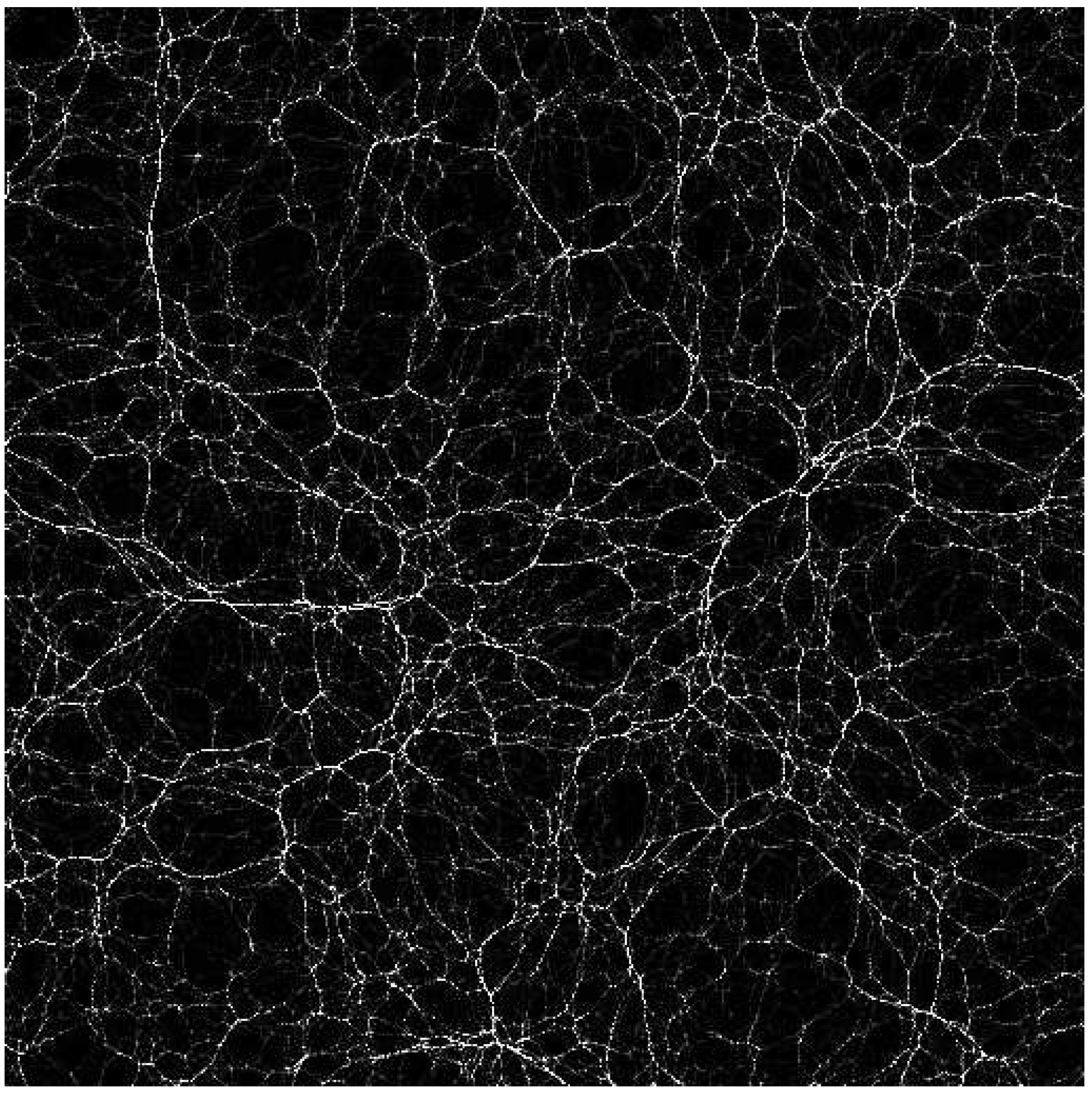
Naturally, we use the zero-redshift (present time) snapshots of either simulation. A representative image of the matter distribution is given by the distribution in a slice, see Figure 2. This slice is prepared as follows. First of all, we focus on the dominant CDM component of the Mare Nostrum simulation. Since the number of particles is very large, it is useful to coarse-grain the particle distribution to obtain a density representation [14,15]. The coarse-graining is carried out by using a mesh of cubes with length such that the average density is one particle per cube [15], so the mesh-cube’s edge is $1/1024$ of the simulation cube’s edge. Furthermore, given that the homogeneity scale is about 3% of the simulation cube’s edge [15], a quarter of a full slice is adequate to perceive the features of the matter distribution (the lower left quarter is taken). In summary, our slice consists of $512\times 512$ mesh-cubes, and the density is given by the number of particles in each one. To each mesh-cube corresponds a pixel in the image, with an intensity proportional to the density in the mesh-cube. In addition, in the slice represented in Figure 2, the density field has been cut off at $\varrho =4$ ($\varrho =1$ is the average density), so that the contrast does not render invisible the pixels corresponding to low-density cubes and one can appreciate the full cosmic-web structure. Indeed, Figure 2 shows a self-similar structure that looks like the structure in Figure 1.

Figure 2. Dark matter slice of Mare Nostrum N-body simulation (cut off at $\varrho =4$).

Figure 2. Dark matter slice of Mare Nostrum N-body simulation (cut off at $\varrho =4$).

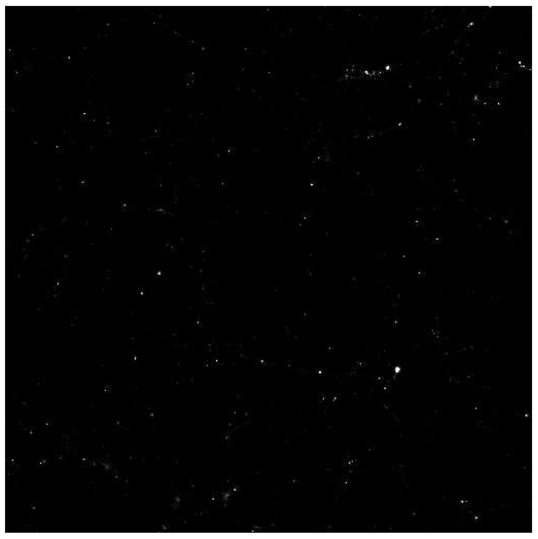
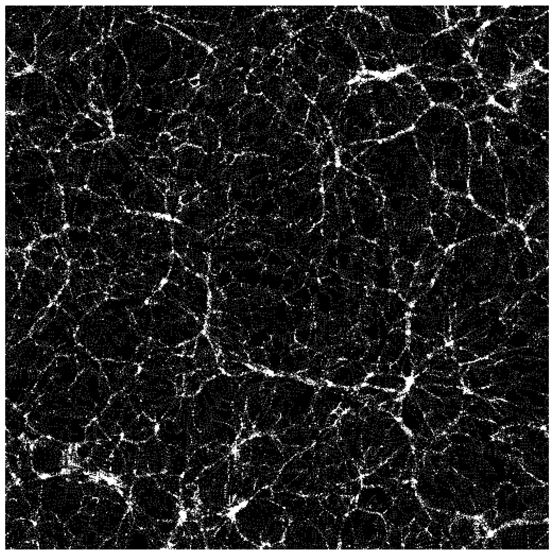
Nevertheless, one can wonder what is the appearance of the full density, namely, including $\varrho >4$. To see this, let us raise the cutoff to $\varrho =256$, a value that is only exceeded by a few mesh-cubes and that, at the same time, preserves some contrast in the picture. Amazingly, this change makes the cosmic-web structure of Figure 2 vanish and the new image, Figure 3, resembles what one can see in a starry night, namely, distinct bright spots with a (small) range of sizes. Naturally, these bright spots must be identified with dark matter halos rather than with stars. To understand the transformation from a cosmic web structure to a distribution of halos of similar size, we must spell out the various scales that play a role in cosmological N-body simulations.

Figure 3. The same slice of Figure 2 but cut off at $\varrho =256$. Notice the halos.

Figure 3. The same slice of Figure 2 but cut off at $\varrho =256$. Notice the halos.

Of course, the first scale is the simulation cube’s edge, but we can refer the remaining scales to it and, hence, assign it the value of unity. The next scale is the discretization length $N^{-1/3}$, namely, the length of the edge of the mesh cube such that there is one particle per cube on average. Naturally, the mesh of these cubes is used for the counts-in-cells and $N^{-1/3}=1/1024$ is the coarse-graining length (in physical units, $0.5h^{-1}$ Mpc, in the Mare Nostrum simulation). There is another scale: the gravity cutoff or softening length, which is necessary to avoid numerical problems when two particles get close and the force between them gets too large. The softening length is of the order of some Kpc, in particular, it is $15h^{-1}$ Kpc in the Mare Nostrum simulation. (In the GIF2 simulation, the discretization length is $0.25h^{-1}$ Mpc and the softening length is $=7h^{-1}$ Kpc, so their ratio is almost the same.) Besides, there are other scales in the initial conditions, but we are only concerned with the scales in the dynamics. In summary, while CDM dynamics is scale free, we see that N-body simulations of it introduce two scales. Therefore, the appearance of halos in Figure 3 must be due to the presence of these scales, which prevent the formation of a truly self-similar cosmic web. Indeed, scale invariance can certainly be measured for scales between the homogeneity scale and the discretization scale [14,15]. In addition, the halos in Figure 3 have sizes of the order of the discretization length, which is the larger of the two scales.

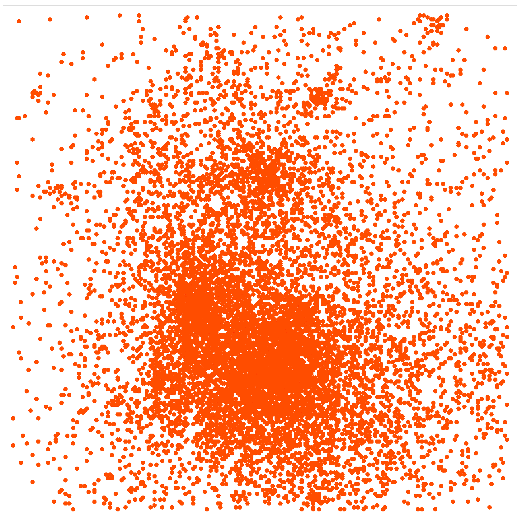
While Figure 2 or Figure 3 show the matter distribution between the homogeneity scale and the discretization scale, they do not show the distribution on smaller scales, that is, they do not show what one might call the mass distribution inside halos. The most populated mesh-cube is located at the position $(380/512,159/512)$ in the slice and contains 2466 particles (to be compared with one per mesh-cube, on average). Nearby cubes are overpopulated as well, so we define the heaviest halo as the one formed by all of them together. To be precise, we choose $4\times 4$ adjacent cubes of the slice and we display the (projected) particle positions in them in Figure 4. Other halos in the slice have a similar aspect. Patently, the matter distribution on these small scales is very different from the cosmic-web distribution between the homogeneity scale and the discretization scale: now we perceive a nearly smooth distribution (this also happens for the GIF2 simulation, naturally). The smoothness of the distribution inside halos is presumably due to the gravity softening. However, the scale that seems to mark the transition from an irregular cosmic-web distribution to a smooth distribution is the discretization scale. The transition over this scale has an even more definite and sharp effect on the statistics of halo masses, as we show next.

Figure 4. Zooming in on the largest halo: $4\times 4$ pixels at position $(0.74,0.31)$ in Figure 3.

Figure 4. Zooming in on the largest halo: $4\times 4$ pixels at position $(0.74,0.31)$ in Figure 3.

4.1. Halo Mass Statistics

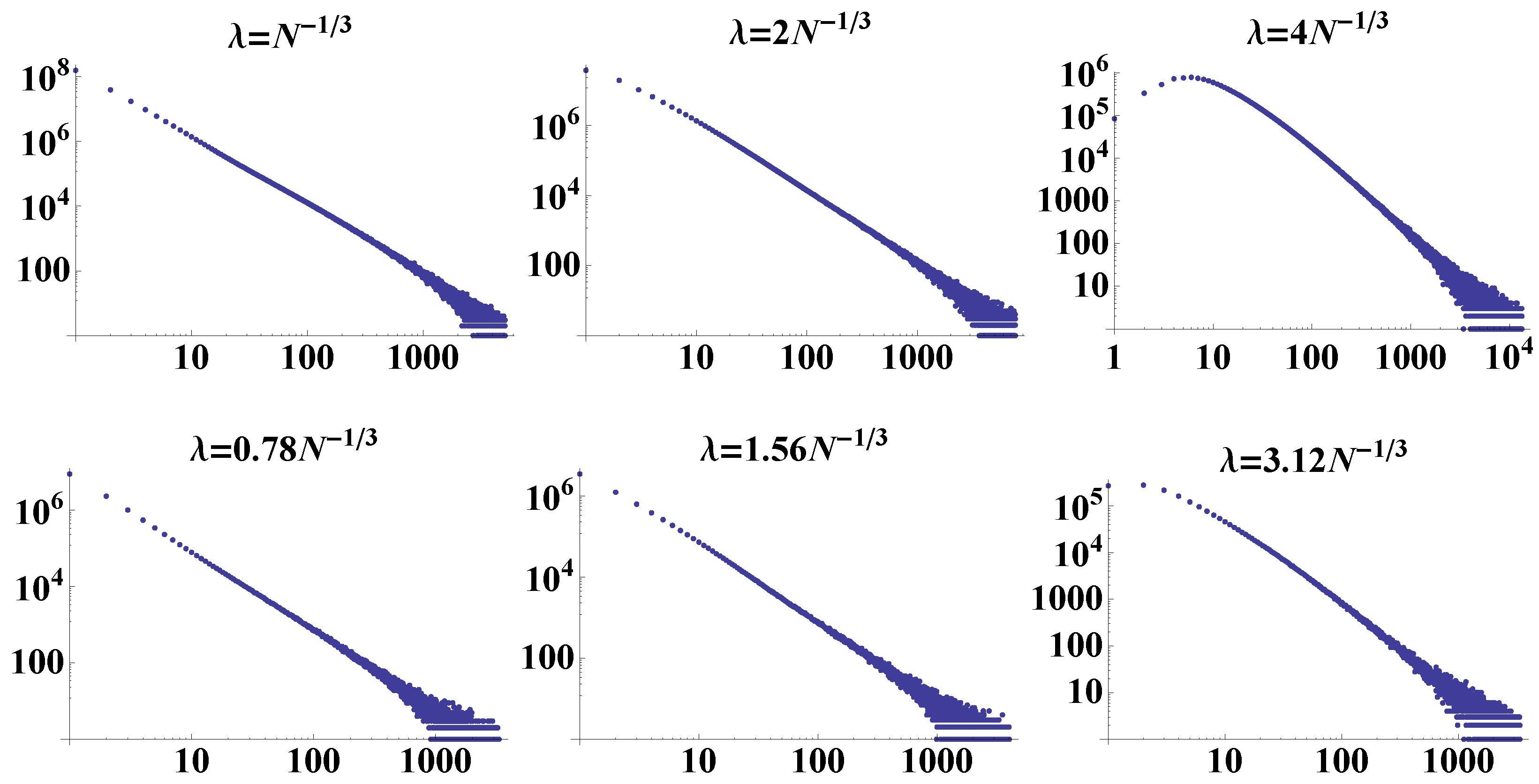
Since we have seen that the halo sizes in N-body simulations are about the discretization scale, it is appropriate to define halos so that they have precisely this size, for the sake of simplification. Then, one can easily measure by counts-in-cells the mass function of halos, namely, the number of halos of a given mass. The halo mass functions of the Mare Nostrum or GIF2 zero-redshift snapshots follow very definite power laws precisely when the halos have the size of the discretization scale [14,15]. This is shown in Figure 5, where the respective constant size halo mass functions for variable size are displayed: power laws for size $N^{-1/3}$ are fulfilled by all halos except the most massive ones. As the halo size increases, the straight line bends, becoming convex from above, as expected in a multifractal distribution [14,15]. On the contrary, as the halo size decreases, the straight line becomes concave from above, because the number of mesh-cubes with few particles must then increase. Notice that the sizes chosen in the GIF2 simulation are not exact multiples of $N^{-1/3}$, in consonance with the characteristics of this simulation and our numerical methods: the GIF2 simulation contains ${400}^3$ dark matter particles and we use powers of 2 [14].

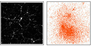
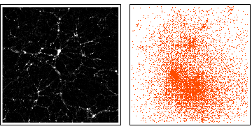
Figure 5. Constant size halo mass functions for variable size λ, for the Mare Nostrum, above, and GIF2, below, $z=0$ snapshots. Abscissas: halo mass; ordinates: number of halos.

Figure 5. Constant size halo mass functions for variable size λ, for the Mare Nostrum, above, and GIF2, below, $z=0$ snapshots. Abscissas: halo mass; ordinates: number of halos.

The power-law mass function of halos at the discretization scale is found in every cosmological N-body simulation that we have analyzed, besides the Mare Nostrum and GIF2 simulations, but we have no simple explanation of it. It can be connected with the Press–Schechter theory of structure formation by spherical collapse of overdensities in a Gaussian distribution, but the power-law exponent is just beyond the allowed range [14,15]. In contrast, the parabola like shape (in a log-log plot) seen on larger scales is explained by a lognormal like model that, in turn, corresponds to a multifractal model of the matter distribution on those scales. This model has been described in detail before (see [14,15] and references therein), so we now restrict ourselves to properties that are relevant with regard to halos.

5. Scale Invariance and Halos

Let us review very briefly the multifractal model of the large-scale structure in cosmological N-body simulations, focusing on the CDM component of the Mare Nostrum simulation. In the multifractal model, the coarse-grained density $\varrho (\mathit{x},r)$ (defined by counts-in-cells or any suitable method), at the point x and for coarse-graining length r, fulfills $\varrho (\mathit{x},r)\sim r^{\alpha (}{{}^x}^{)}{}^{-3}$, where $\alpha \ge 0$ (see [16] for a precise definition). Consequently, the point density ${lim}_{r\to 0}\varrho (\mathit{x},r)$ is finite and non-vanishing only if $\alpha =3$, while it is infinite for $\alpha <3$, and zero for $\alpha >3$. Therefore, it is natural to associate points x such that $0\le \alpha \left(\mathit{x}\right)<3$, namely, density singularities, with halos and points such that $\alpha \left(\mathit{x}\right)>3$ with cosmic voids. At any rate, multifractality is ensured by the power-law behavior of the density with respect to the coarse-graining length or, equivalently, by the power-law behavior of the statistical moments $M_q\left(r\right)$ of the distribution [16]. A multifractal can be characterized by its multifractal spectrum, namely, the fractal dimension $f\left(\alpha \right)$ of the set of points x with exponent α. Notice that the multifractal spectrum can be defined for any distribution with singularities, not just for self-similar distributions. However, multifractal spectra of self-similar distributions have typical parabola like shapes [16,17].

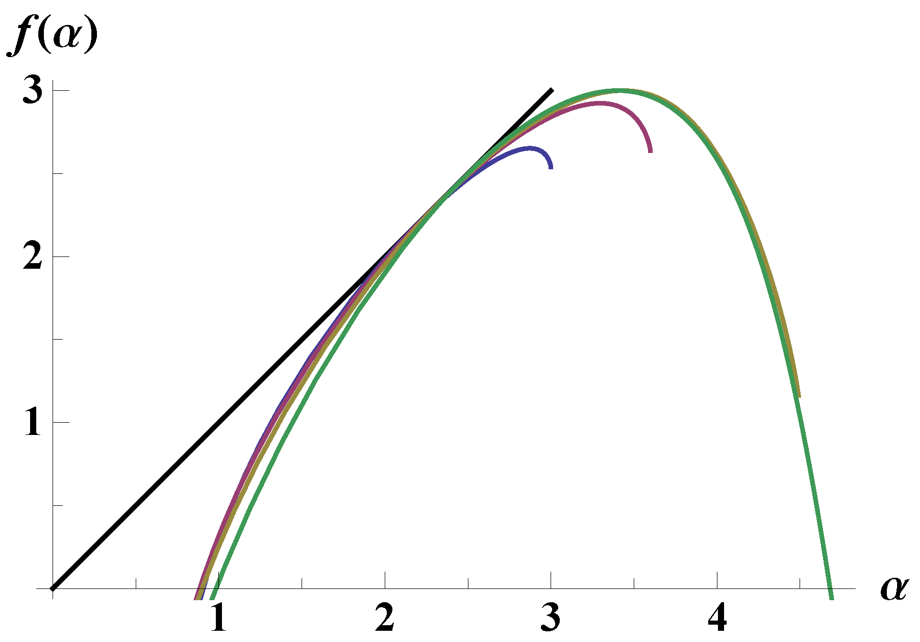
One proof of multifractality consists in computing the coarse multifractal spectrum for several coarse-graining lengths r and showing that it does not depend on r. We reproduce in Figure 6 the coarse multifractal spectrum of the dark matter in the Mare Nostrum simulation for $r=\{1,2,4,8\}\times N^{-1/3}$, which cover most of the scaling range [15]. The extent of the scaling range and the transition to homogeneity are better perceived in the scaling of moments $M_q\left(r\right)$ [15]. The scaling range, which goes from the discretization length (or somewhat below) to the homogeneity scale, extends over two decades, at the most.

Figure 6. Multifractal spectra of the dark matter in the Mare Nostrum simulation, for $r=\{1,2,4,8\}\times N^{-1/3}$ (blue, red, brown and green, respectively).

Figure 6. Multifractal spectra of the dark matter in the Mare Nostrum simulation, for $r=\{1,2,4,8\}\times N^{-1/3}$ (blue, red, brown and green, respectively).

Unfortunately, the scaling range in three-dimensional N-body simulations cannot be very large, for the time being. In contrast, one-dimensional cosmological N-body simulations with moderate N can reach truly compelling scaling ranges: the simulations of Miller et al. [18], with $N\le 2^{18}\simeq 2.6\times {10}^5$, and of Joyce and Sicard [19], with $N={10}^5$, reach almost 4 decades! Moreover, the analysis by Joyce and Sicard of the “halos” formed in their simulation has led them to state, regarding three-dimensional halos, that CDM halos are “not well modeled as smooth objects” and that “the supposed ‘universality’ of [halo] profiles is, like apparent smoothness, an artifact of poor numerical resolution”. These conclusions agree with the conclusions from our own analyses in three dimensions [3,14,15]: if we are to preserve the concept of CDM halos, they are to be defined as grainy structures in a self-similar distribution rather than smooth structures with a range of sizes.

A different but very interesting demonstration of, on the one hand, scale invariance and of, on the other hand, the discreteness limitations of cosmological N-body simulations is provided by the work of Gottlöber et al. [20]. The purpose of their work is to assess the problem of the emptiness of cosmic voids by means of N-body simulations. To do this, Gottlöber et al. [20] performed a low resolution simulation and then resimulate voids with high resolution, namely, with the resolution corresponding to replacing each particle with 512 particles. Naturally, they find that the voids are no longer empty and, furthermore, the high-resolution dark matter distribution inside large voids is such that “haloes are arranged in a pattern, which looks like a miniature universe.” In other words, Gottlöber et al. find that a higher resolution brings out in a void the invisible structure below the discretization scale, demonstrating self-similarity of the full structure. One can infer that a resimulation of halos with higher resolution must bring out as well their grainy, self-similar structure.

6. Discussion and Conclusions

It seems inevitable to conclude that the presence of an intrinsic scale in cosmological N-body simulations, namely, the discreteness scale $N^{-1/3}$, severely affects the type of mass distribution that is produced below that scale, to the extent that the smooth halos with a range of sizes about that scale that are commonly seen in these simulations are probably an artifact of insufficient resolution.

The problems of cosmological N-body simulations below the discreteness scale have already been noticed by Splinter et al. [4]: their comparison of results of various N-body simulations reveals that “codes never agree well below the mean comoving interparticle separation” (which is another name for the discreteness scale). Therefore, one might think that the smoothness of halos that is seen on these small scales should have been questioned before. Probably, this has not occurred (or has had no consequences) because of the popularity of the spherical collapse model. However, now it appears that this model does not necessarily predict smooth spherical halos and, in addition, its range of application is far more restricted than usually assumed.

In fact, the adhesion model is more adequate than the spherical collapse model to provide a general description of large scale structure, namely, to produce the typical cosmic web structure perceived in both CDM simulations and observations of the galaxy distribution. The cosmic web is self-similar, so the adhesion model suggests that the size of halos or, in general, the size of cosmic-web structures is determined by small-scale processes that can be lumped into an effective viscosity that breaks the scale invariance. The question is, of course, how such small-scale processes determine the scale at which scale invariance is broken and how this scale compares with the discreteness scale $N^{-1/3}>0.2h^{-1}$ Mpc (generally).

First of all, let us remark that the real CDM is probably discrete. Indeed, current models of CDM favor a WIMP composition. Neutralinos, for example, may have a mass $<1$ TeV. Therefore, comparing with the mass resolution of cosmological N-body simulations (e.g., $8.24\times {10}^9{h}^{-1}$ M${}_{\odot }$ in the Mare Nostrum simulation), there is such a huge factor (${10}^{64}$ in the Mare Nostrum simulation) that the CDM distribution on astrophysical scales is continuous, in practice, and, hence, N-body simulations can in no way reproduce the real CDM dynamics on small scales.

We could also consider that the scale invariance of CDM dynamics is broken on small scales by an aspect of it that is not taken into account by N-body simulations: the collapse of CDM overdensities eventually produces densities and velocities that make Newtonian physics invalid and require relativistic physics. In general relativity, a mass has an associated length scale, namely, its Schwarschild radius. Consequently, in the “top-hat” collapse model, for example, there is an intrinsic scale, which, in contrast with the usually assumed scale, is not arbitrary and, furthermore, is independent of the initial conditions. Naturally, this new scale arises in connection with supermassive black hole formation and, arguably, the size of these black holes is not relevant on cosmological scales.

In conclusion, the CDM dynamics does not seem to generate any small scale that is cosmologically relevant. Thus, it seems natural to either define a sort of scale invariant halos [3,14,15] or to turn to the baryon physics. However, it is not easy to think of a definite scale in the baryonic physics that marks the end of scale invariance. As a matter of fact, the gas in the Mare Nostrum simulation follows the same scaling laws as the CDM does, despite the presence of biasing [15]. At any rate, the modeling of baryonic physics in cosmological N-body simulations is still in its infancy [11]. What seems clear is that the standard conclusions about smooth halos with a range of sizes drawn from state-of-the-art N-body simulations, especially, CDM-only simulations, must be reassessed.