
Improved Deep Convolutional Neural Network to Classify Osteoarthritis from Anterior Cruciate Ligament Tear Using Magnetic Resonance Imaging

 ,
, 
 and
and
Abstract
:1. Introduction
2. Materials and Methods
2.1. Data Collection Description
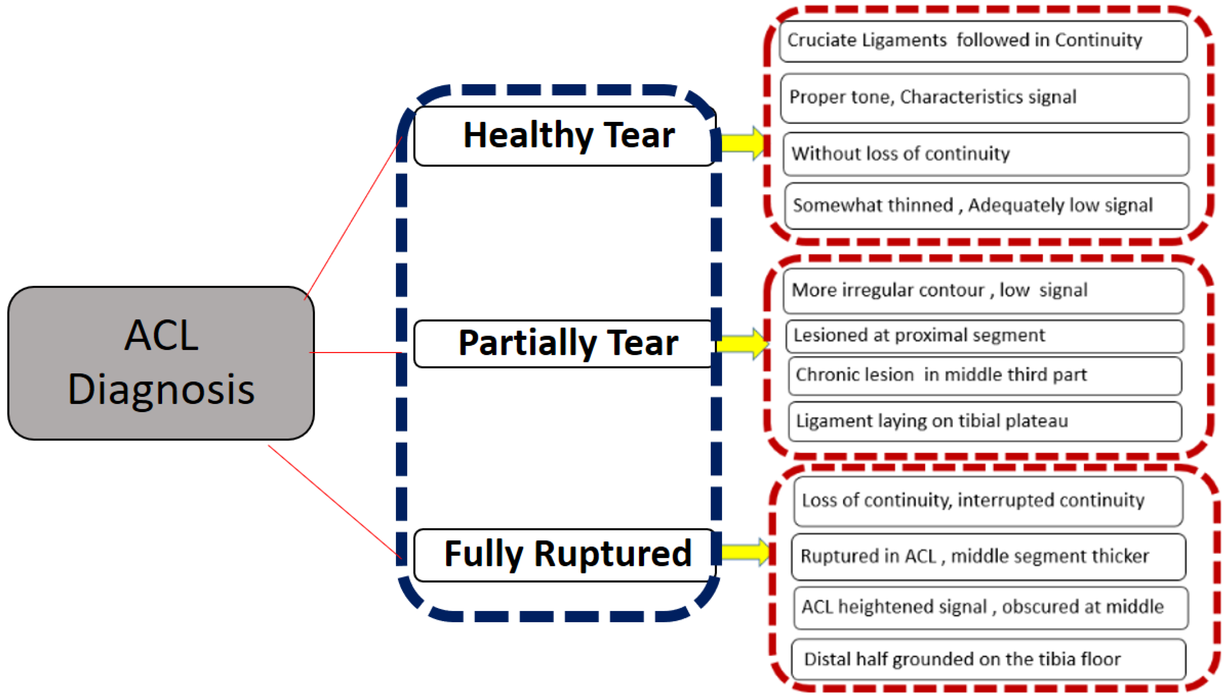
2.2. Data Exclusion and Labelling Criteria
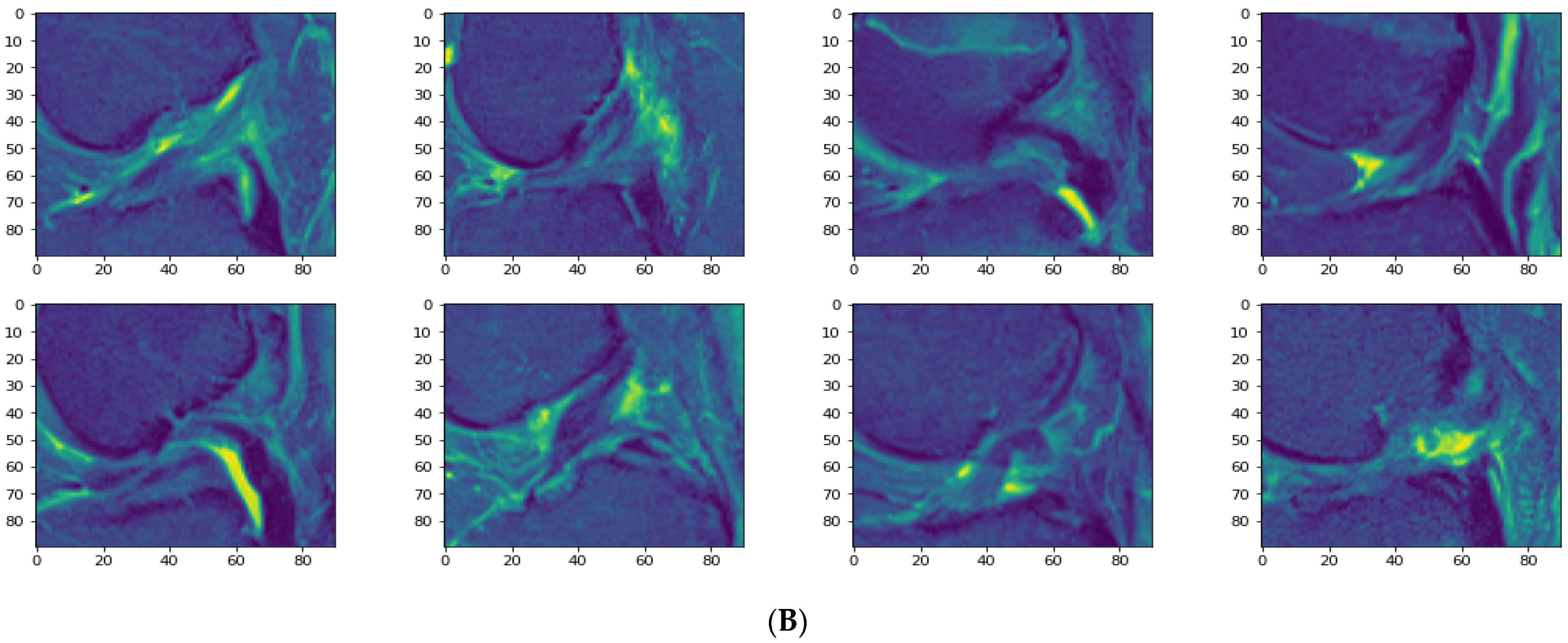
2.3. Data Pre-Processing
2.4. Convolutional Neural Network Methodology
- 1.
- Convolutional Layer
- 2.
- Activation Layer
- 3.
- Pooling Layer
- 4.
- Fully Connected Layer
- 5.
- Output Layer
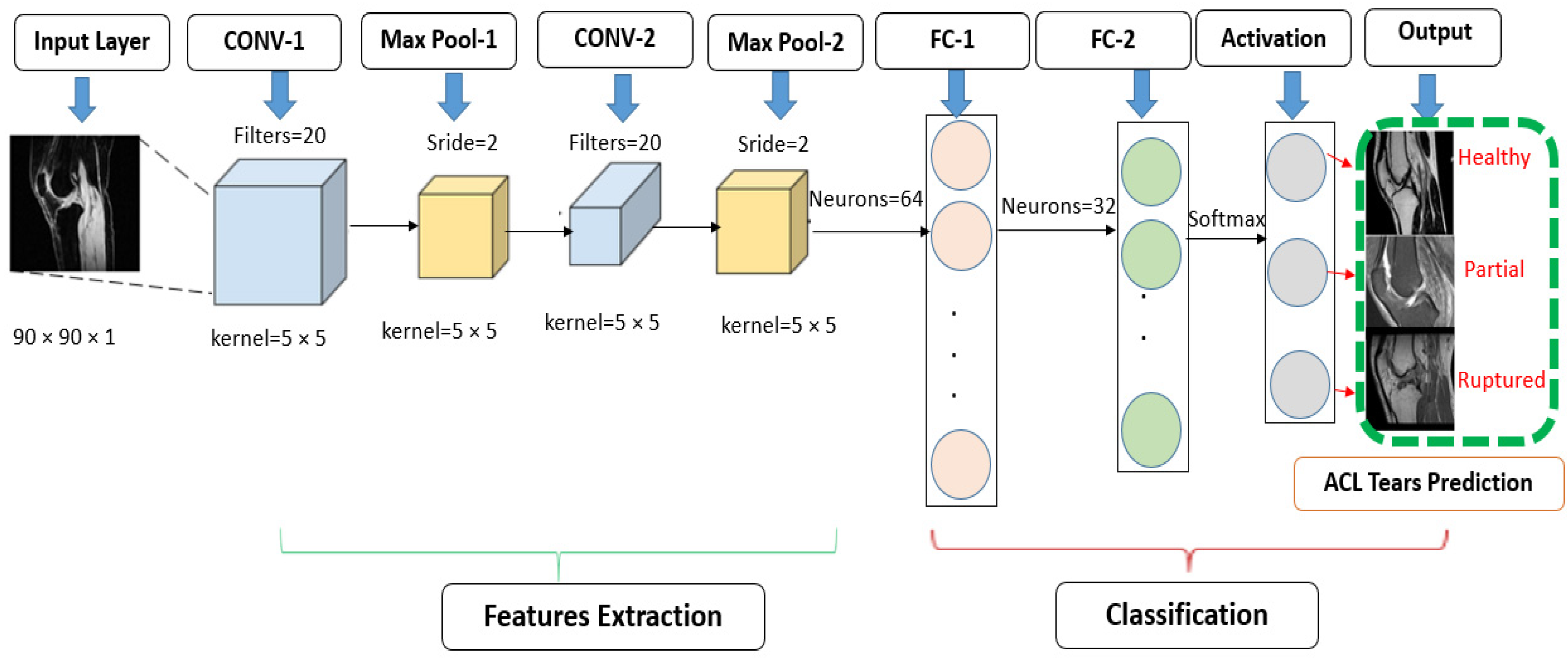
2.4.1. Standard CNN Modified Architecture
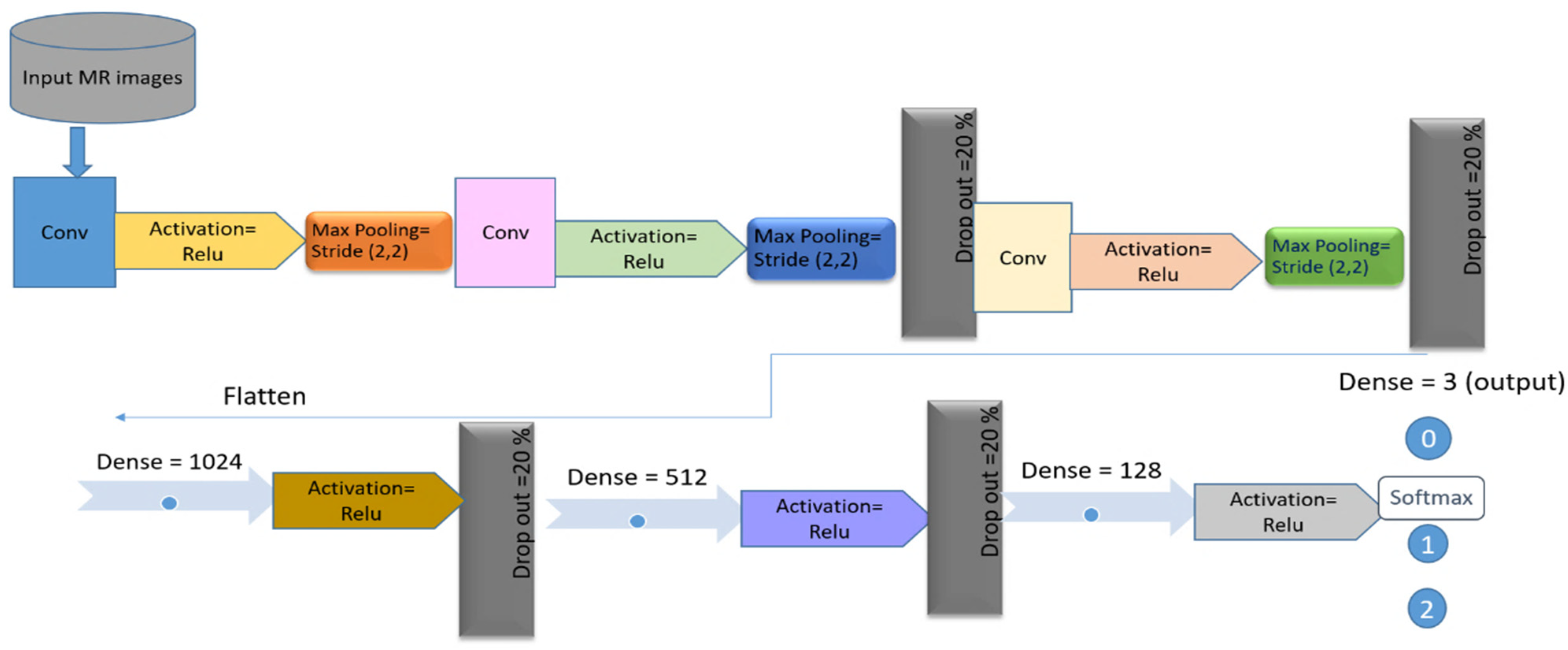
2.4.2. Customized Convolutional Neural Network
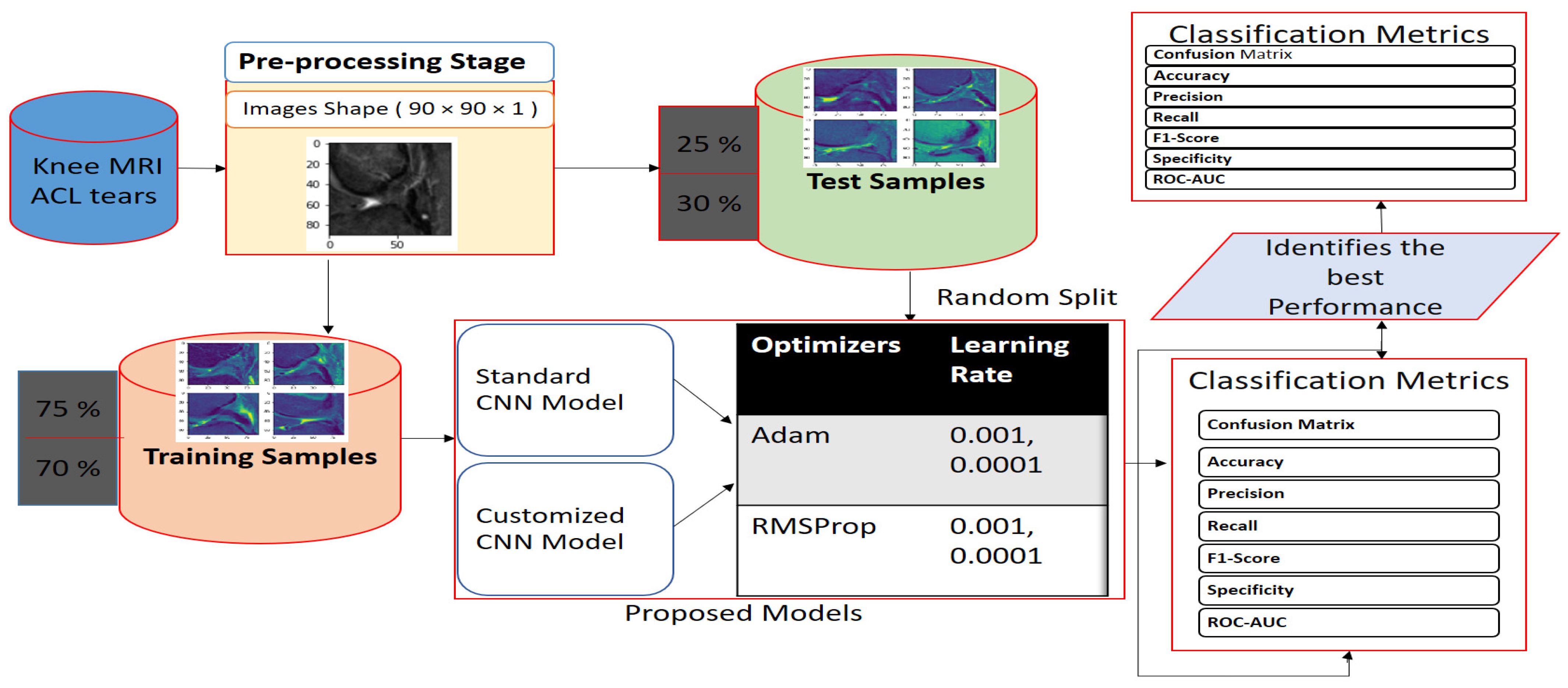
2.5. Proposed Work Framework
3. Experimental Results
3.1. Implementation Details
3.2. Train and Test Random Splitting
3.3. Hyperparameter Adjustments of our Models
- The RMSProp optimizer tries to dimple the auscultations. It fixes the convergence problem to global minima in the adaptive gradient (AdaGrad) optimizer by accumulating only the gradients from the recent iterations. RMSprop chooses different learning rates for each parameter. RMSprop updates as mentioned in Equation (5). The value of the beta decay rate is close to 0.0001. The weights are updated as shown in Equation (6).
- Adam is a well-known optimizer with good performance when it comes to classifying images in CNNs. It is a variant of a combination of RMSprop and momentum. It uses an estimation of the first and second momentum of gradients to adapt the learning rate for each weight of the neural network. Adam also makes use of the average of the second moments of the gradients. The algorithm calculates an exponential moving average of the gradient and the squared gradient, and the parameters beta1 and beta2 control the decay rates of these moving averages in Equations (7)–(9).
3.4. Evaluation Metrics
- 1.
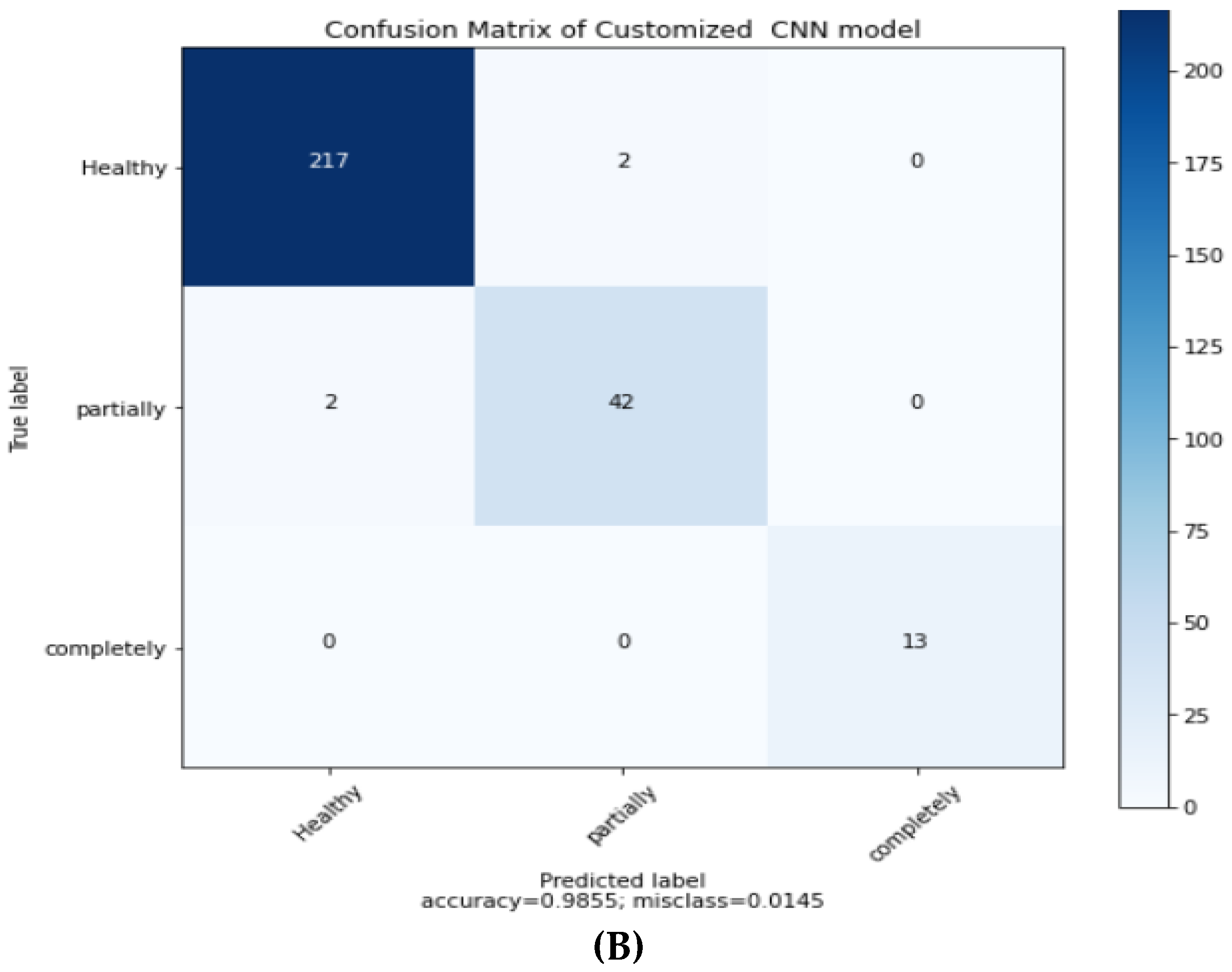
- Confusion matrix
- 2.
- Accuracy
- 3.
- Precision (or positive predicted value)
- 4.
- Recall (or sensitivity, hit rate, or true positive rate)
- 5.
- Specificity or true negative rate
- 6.
- F1 score
- 7.
- Categorical cross-entropy
- 8.
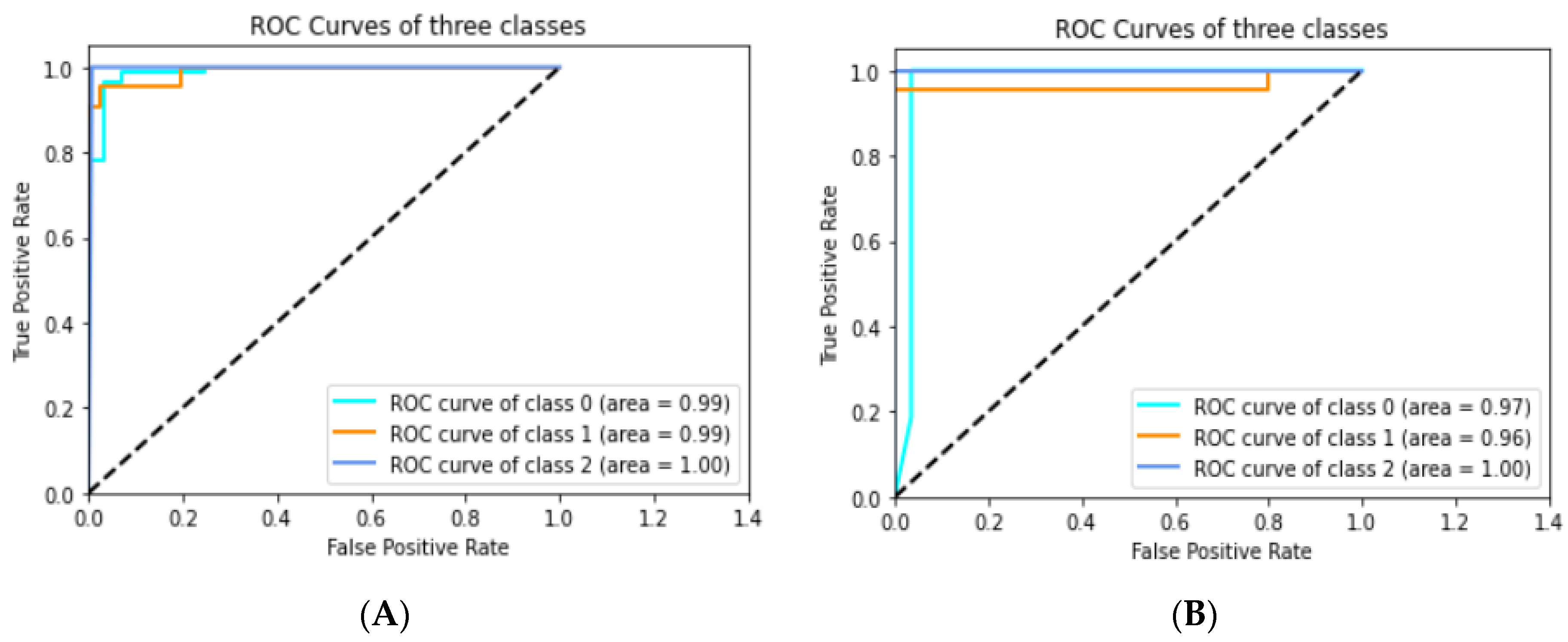
- ROC AUC
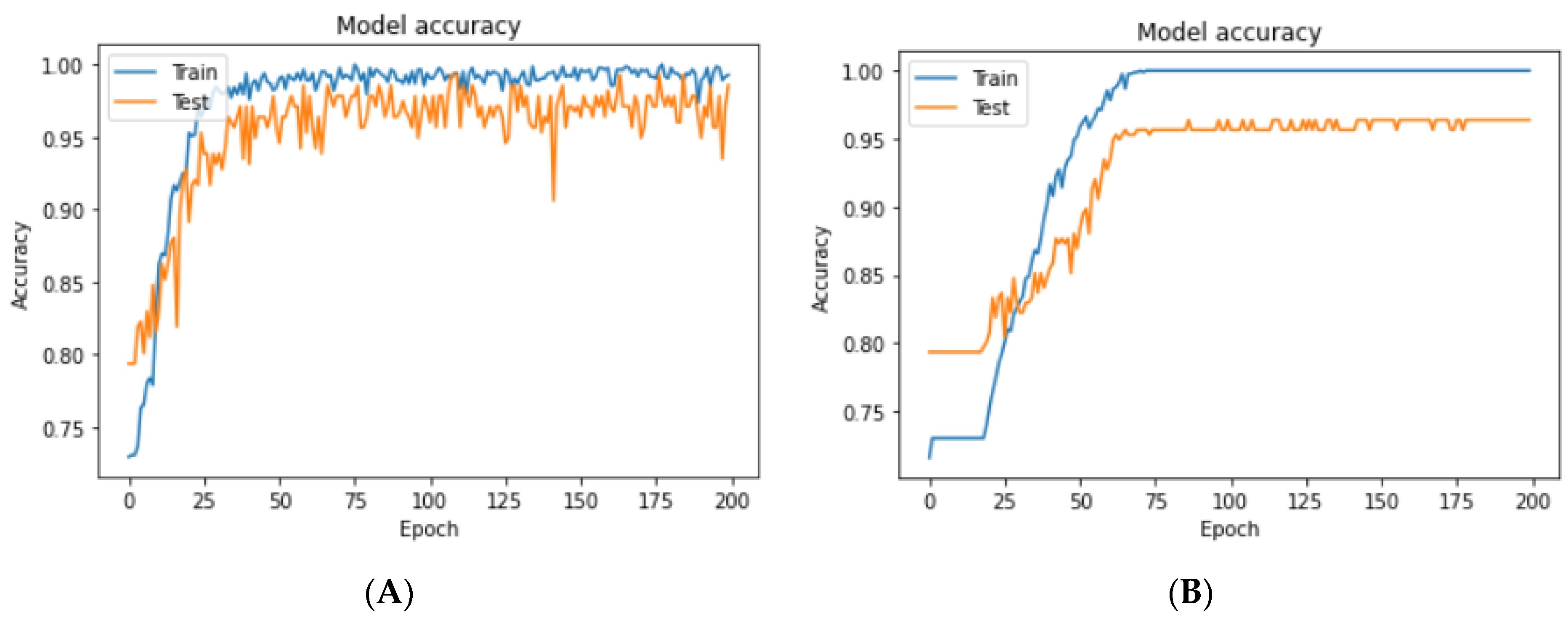
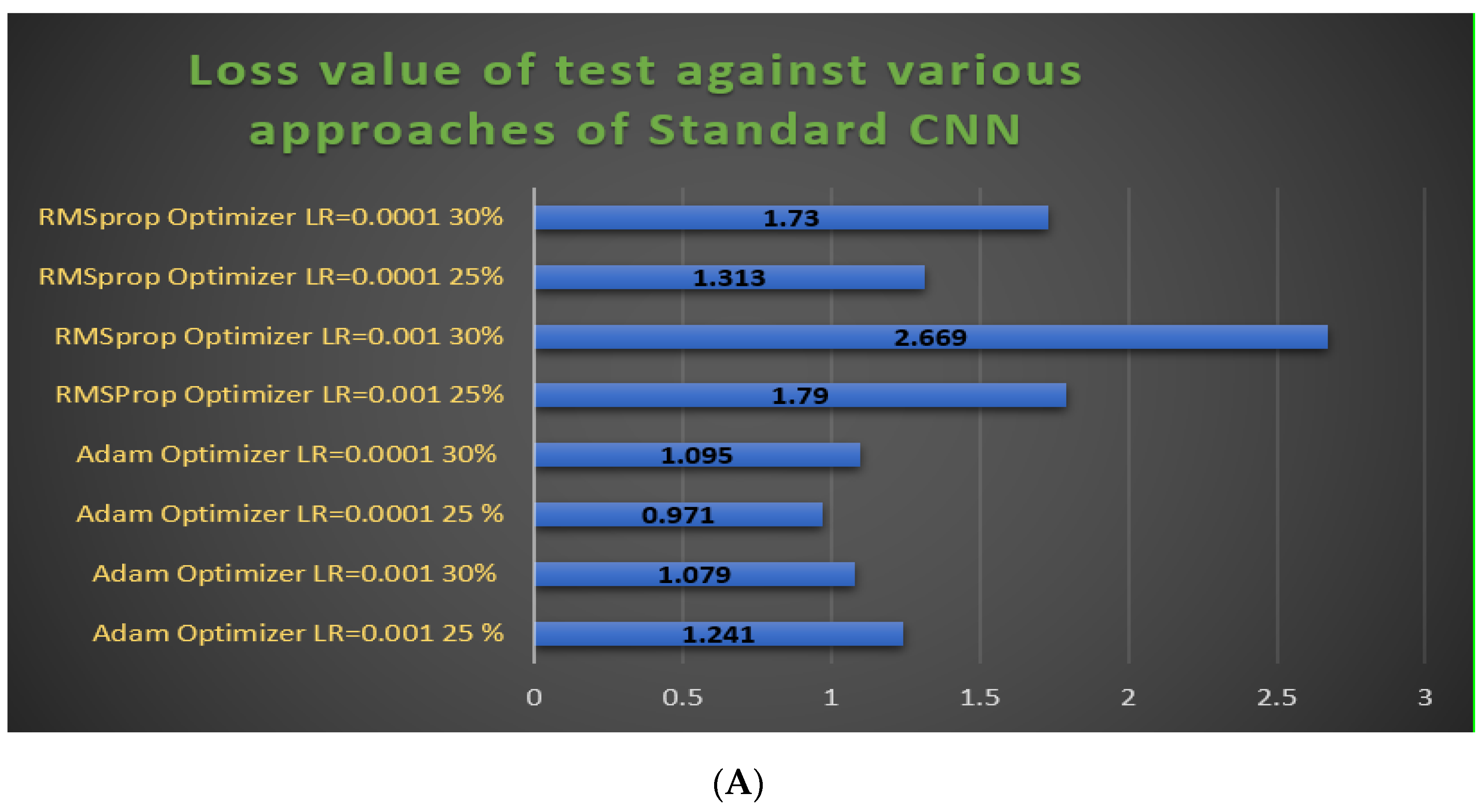
3.4.1. Experimental Prediction Performance of Standard CNN Model
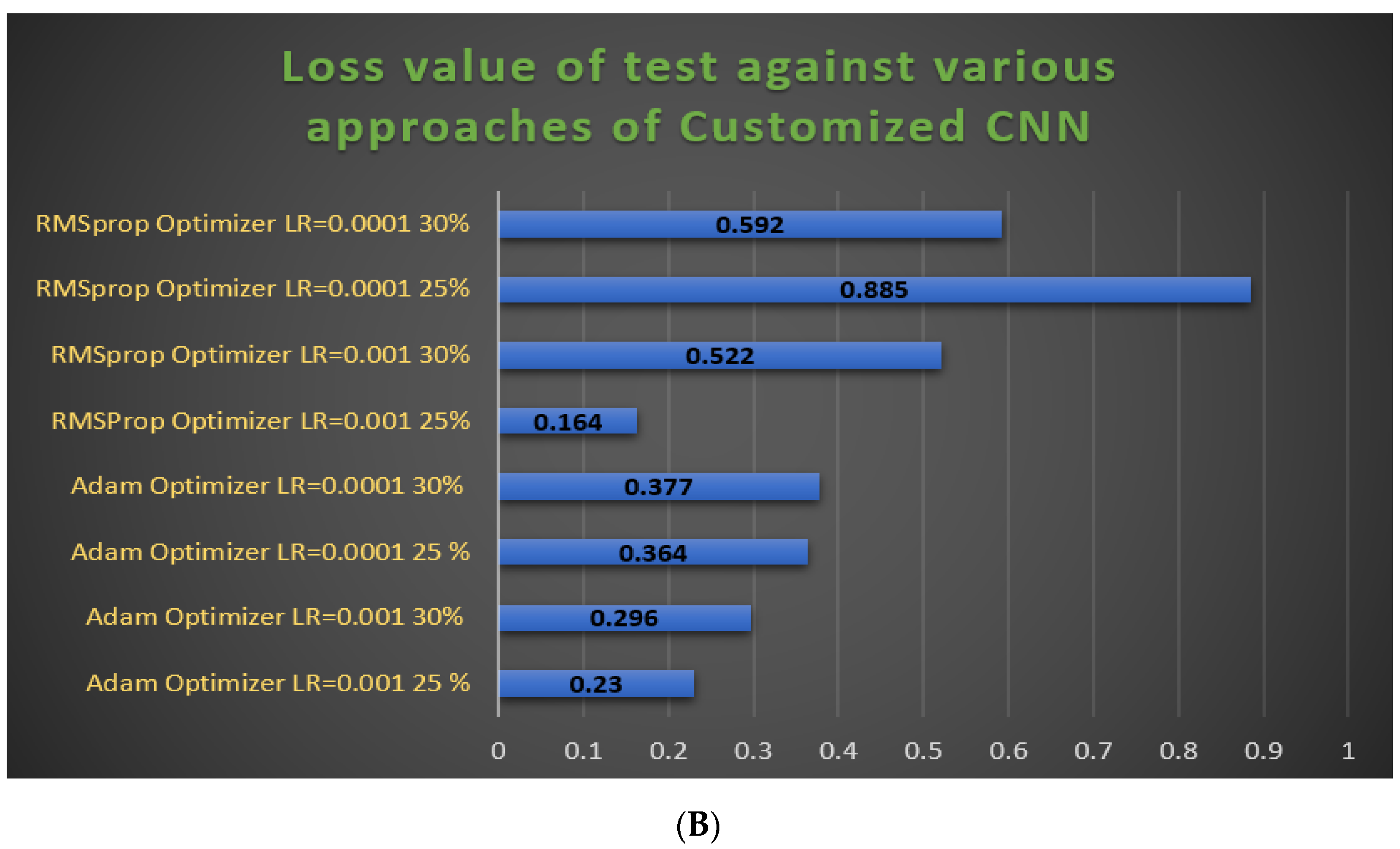
3.4.2. Experimental Prediction Performance of the Customized CNN Model
3.4.3. Result Comparison between Standard and Customized CNN Approaches
4. Discussion
5. Conclusions
Author Contributions
Funding
Institutional Review Board Statement
Informed Consent Statement
Data Availability Statement
Conflicts of Interest
References
- Hasegawa, A.; Otsuki, S.; Pauli, C.; Miyaki, S.; Patil, S.; Steklov, N.; Kinoshita, M.; Koziol, J.; D’Lima, D.D.; Lotz, M.K. Anterior cruciate ligament changes in the human knee joint in aging and osteoarthritis. Arthritis Rheum. 2012, 64, 696–704. [Google Scholar] [CrossRef] [Green Version]
- Grothues, S.A.G.A.; Radermacher, K. Variation of the Three-Dimensional Femoral J-Curve in the Native Knee. J. Pers. Med. 2021, 11, 592. [Google Scholar] [CrossRef] [PubMed]
- Watkins, L.E.; Rubin, E.B.; Mazzoli, V.; Uhlrich, S.D.; Desai, A.D.; Black, M.; Ho, G.K.; Delp, S.L.; Levenston, M.E.; Beaupre, G.S.; et al. Rapid volumetric gagCEST imaging of knee articular cartilage at 3 T: Evaluation of improved dynamic range and an osteoarthritic population. NMR Biomed. 2020, 33, e4310. [Google Scholar] [CrossRef] [PubMed]
- Hong, S.H.; Choi, J.Y.; Lee, G.K.; Choi, J.A.; Chung, H.W.; Kang, H.S. Grading of anterior cruciate ligament injury: Diagnostic efficacy of oblique coronal magnetic resonance imaging of the knee. J. Comput. Assist. Tomogr. 2003, 27, 814–819. [Google Scholar] [CrossRef] [PubMed]
- Poon, Y.-Y.; Yang, J.C.-S.; Chou, W.-Y.; Lu, H.-F.; Hung, C.-T.; Chin, J.-C.; Wu, S.-C. Is There an Optimal Timing of Adductor Canal Block for Total Knee Arthroplasty?—A Retrospective Cohort Study. J. Pers. Med. 2021, 11, 622. [Google Scholar] [CrossRef]
- Anam, M.; Ponnusamy, V.; Hussain, M.; Nadeem, M.W.; Javed, M.; Goh, H.G.; Qadeer, S. Osteoporosis Prediction for Trabecular Bone using Machine Learning: A Review. Comput. Mater. Contin. 2021, 67, 89–105. [Google Scholar] [CrossRef]
- Johnson, V.L.; Guermazi, A.; Roemer, F.W.; Hunter, D.J. Comparison in knee osteoarthritis joint damage patterns among individuals with an intact, complete and partial anterior cruciate ligament rupture. Int. J. Rheum. Dis. 2017, 20, 1361–1371. [Google Scholar] [CrossRef] [PubMed]
- Suter, L.G.; Smith, S.R.; Katz, J.N.; Englund, M.; Hunter, D.J.; Frobell, R.; Losina, E. Projecting lifetime risk of symptomatic knee osteoarthritis and total knee replacement in individuals sustaining a complete anterior cruciate ligament tear in early adulthood. Arthritis Care Res. 2017, 69, 201–208. [Google Scholar]
- Amin, J.; Sharif, M.; Raza, M.; Saba, T.; Anjum, M.A. Brain tumor detection using statistical and machine learning method. Comput. Methods Programs Biomed. 2019, 177, 69–79. [Google Scholar]
- Otsubo, H.; Akatsuka, Y.; Takashima, H.; Suzuki, T.; Suzuki, D.; Kamiya, T.; Ikeda, Y.; Matsumura, T.; Yamashita, T.; Shino, K. MRI depiction and 3D visualization of three anterior cruciate ligament bundles. Clin. Anat. 2017, 30, 276–283. [Google Scholar] [CrossRef]
- Vaishya, R.; Okwuchukwu, M.C.; Agarwal, A.K.; Vijay, V. Does Anterior Cruciate Ligament Reconstruction prevent or initiate Knee Osteoarthritis?—A critical review. J. Arthrosc. Jt. Surg. 2019, 6, 133–136. [Google Scholar] [CrossRef]
- Hill, C.L.; Seo, G.S.; Gale, D.; Totterman, S.; Gale, M.E.; Felson, D.T. Cruciate ligament integrity in osteoarthritis of the knee. Arthritis Rheum. 2005, 52, 794–799. [Google Scholar] [CrossRef]
- Hernandez-Molina, G.; Guermazi, A.; Niu, J.; Gale, D.; Goggins, J.; Amin, S.; Felson, D.T. Central bone marrow lesions in symptomatic knee osteoarthritis and their relationship to anterior cruciate ligament tears and cartilage loss. Arthritis Rheum. 2008, 58, 130–136. [Google Scholar] [CrossRef] [PubMed] [Green Version]
- Nenezić, D.; Kocijancic, I. The value of the sagittal-oblique MRI technique for injuries of the anterior cruciate ligament in the knee. Radiol. Oncol. 2013, 47, 19–25. [Google Scholar] [CrossRef]
- Iqbal, S.; Khan, M.U.G.; Saba, T.; Mehmood, Z.; Javaid, N.; Rehman, A.; Abbasi, R. Deep learning model integrating features and novel classifiers fusion for brain tumor segmentation. Microsc. Res. Tech. 2019, 82, 1302–1315. [Google Scholar] [PubMed]
- Sadad, T.; Rehman, A.; Munir, A.; Saba, T.; Tariq, U.; Ayesha, N.; Abbasi, R. Brain tumor detection and multi-classification using advanced deep learning techniques. Microsc. Res. Tech. 2021, 84, 1296–1308. [Google Scholar]
- Qiu, B.; van der Wel, H.; Kraeima, J.; Glas, H.H.; Guo, J.; Borra, R.J.H.; Witjes, M.J.H.; van Ooijen, P.M.A. Automatic Segmentation of Mandible from Conventional Methods to Deep Learning—A Review. J. Pers. Med. 2021, 11, 629. [Google Scholar] [CrossRef] [PubMed]
- Mujahid, A.; Awan, M.J.; Yasin, A.; Mohammed, M.A.; Damaševičius, R.; Maskeliūnas, R.; Abdulkareem, K.H. Real-Time Hand Gesture Recognition Based on Deep Learning YOLOv3 Model. Appl. Sci. 2021, 11, 4164. [Google Scholar] [CrossRef]
- Jamal, A.; Alkawaz, M.H.; Rehman, A.; Saba, T. Retinal imaging analysis based on vessel detection. Microsc Res. Tech. 2017, 80, 799–811. [Google Scholar] [CrossRef]
- Mittal, A.; Kumar, D.; Mittal, M.; Saba, T.; Abunadi, I.; Rehman, A.; Roy, S. Detecting Pneumonia Using Convolutions and Dynamic Capsule Routing for Chest X-ray Images. Sensors 2020, 20, 1068. [Google Scholar] [CrossRef] [Green Version]
- Gupta, M.; Jain, R.; Arora, S.; Gupta, A.; Javed Awan, M.; Chaudhary, G.; Nobanee, H. AI-enabled COVID-9 Outbreak Analysis and Prediction: Indian States vs. Union Territories. Comput. Mater. Contin. 2021, 67, 933–950. [Google Scholar] [CrossRef]
- Awan, M.J.; Bilal, M.H.; Yasin, A.; Nobanee, H.; Khan, N.S.; Zain, A.M. Detection of COVID-19 in Chest X-ray Images: A Big Data Enabled Deep Learning Approach. Int. J. Environ. Res. Public Health 2021, 18, 10147. [Google Scholar] [PubMed]
- Rehman, A.; Abbas, N.; Saba, T.; Rahman, S.I.U.; Mehmood, Z.; Kolivand, H. Classification of acute lymphoblastic leukemia using deep learning. Microsc. Res. Tech. 2018, 81, 1310–1317. [Google Scholar] [CrossRef] [PubMed]
- Abbas, N.; Saba, T.; Mehmood, Z.; Rehman, A.; Islam, N.; Ahmed, K.T. An automated nuclei segmentation of leukocytes from microscopic digital images. Pak. J. Pharm. Sci. 2019, 32, 2123–2138. [Google Scholar] [PubMed]
- Ali, Y.; Farooq, A.; Alam, T.M.; Farooq, M.S.; Awan, M.J.; Baig, T.I. Detection of schistosomiasis factors using association rule mining. IEEE Access 2019, 7, 186108–186114. [Google Scholar]
- Khan, S.A.; Nazir, M.; Khan, M.A.; Saba, T.; Javed, K.; Rehman, A.; Akram, T.; Awais, M. Lungs nodule detection framework from computed tomography images using support vector machine. Microsc. Res. Tech. 2019, 82, 1256–1266. [Google Scholar] [CrossRef] [PubMed]
- Saba, T. Automated lung nodule detection and classification based on multiple classifiers voting. Microsc. Res. Tech. 2019, 82, 1601–1609. [Google Scholar] [CrossRef]
- Nagi, A.T.; Awan, M.J.; Javed, R.; Ayesha, N. A Comparison of Two-Stage Classifier Algorithm with Ensemble Techniques On Detection of Diabetic Retinopathy. In Proceedings of the 2021 1st International Conference on Artificial Intelligence and Data Analytics (CAIDA), Riyadh, Saudi Arabia, 6–7 April 2021; pp. 212–215. [Google Scholar]
- Rad, A.E.; Rahim, M.S.M.; Rehman, A.; Altameem, A.; Saba, T.J.I.T.R. Evaluation of current dental radiographs segmentation approaches in computer-aided applications. IETE Tech. Rev. 2013, 30, 210–222. [Google Scholar] [CrossRef] [Green Version]
- Saba, T.; Akbar, S.; Kolivand, H.; Bahaj, S.A. Automatic detection of papilledema through fundus retinal images using deep learning. Microsc. Res. Tech. 2021, in press. [Google Scholar]
- Seok, J.; Yoon, S.; Ryu, C.H.; Kim, S.K.; Ryu, J.; Jung, Y.S. A Personalized 3D-Printed Model for Obtaining Informed Consent Process for Thyroid Surgery: A Randomized Clinical Study Using a Deep Learning Approach with Mesh-Type 3D Modeling. J. Pers. Med. 2021, 11, 574. [Google Scholar] [CrossRef] [PubMed]
- Javed, R.; Saba, T.; Humdullah, S.; Jamail, N.S.M.; Awan, M.J. An Efficient Pattern Recognition Based Method for Drug-Drug Interaction Diagnosis. In Proceedings of the 2021 1st International Conference on Artificial Intelligence and Data Analytics (CAIDA), Riyadh, Saudi Arabia, 6–7 April 2021; pp. 221–226. [Google Scholar]
- Khan, M.A.; Lali, I.U.; Rehman, A.; Ishaq, M.; Sharif, M.; Saba, T.; Zahoor, S.; Akram, T. Brain tumor detection and classification: A framework of marker-based watershed algorithm and multilevel priority features selection. Microsc. Res. Tech. 2019, 82, 909–922. [Google Scholar] [CrossRef] [PubMed]
- Khan, A.R.; Khan, S.; Harouni, M.; Abbasi, R.; Iqbal, S.; Mehmood, Z. Brain tumor segmentation using K-means clustering and deep learning with synthetic data augmentation for classification. Microsc. Res. Tech. 2021. [Google Scholar] [CrossRef]
- Rehman, A.; Khan, M.A.; Saba, T.; Mehmood, Z.; Tariq, U.; Ayesha, N. Microscopic brain tumor detection and classification using 3D CNN and feature selection architecture. Microsc. Res. Tech. 2021, 84, 133–149. [Google Scholar] [CrossRef]
- Nabeel, M.; Majeed, S.; Awan, M.J.; Muslih-ud-Din, H.; Wasique, M.; Nasir, R. Review on Effective Disease Prediction through Data Mining Techniques. Int. J. Electr. Eng. Inform. 2021, 13, 717–733. [Google Scholar] [CrossRef]
- Norouzi, A.; Rahim, M.S.M.; Altameem, A.; Saba, T.; Rad, A.E.; Rehman, A.; Uddin, M. Medical image segmentation methods, algorithms, and applications. IETE Tech. Rev. 2014, 31, 199–213. [Google Scholar]
- Afza, F.; Khan, M.A.; Sharif, M.; Rehman, A. Microscopic skin laceration segmentation and classification: A framework of statistical normal distribution and optimal feature selection. Microsc. Res. Tech. 2019, 82, 1471–1488. [Google Scholar] [CrossRef] [PubMed]
- Rakhmadi, A.; Othman, N.Z.S.; Bade, A.; Rahim, M.S.M.; Amin, I.M. Connected component labeling using components neighbors-scan labeling approach. J. Comput. Sci. 2010, 6, 1099. [Google Scholar] [CrossRef] [Green Version]
- Rad, A.E.; Rahim, M.S.M.; Kolivand, H.; Amin, I.B.M. Morphological region-based initial contour algorithm for level set methods in image segmentation. Multimed. Tools Appl. 2017, 76, 2185–2201. [Google Scholar]
- Stajduhar, I.; Mamula, M.; Miletic, D.; Unal, G. Semi-automated detection of anterior cruciate ligament injury from MRI. Comput. Methods Programs Biomed. 2017, 140, 151–164. [Google Scholar] [CrossRef]
- Bien, N.; Rajpurkar, P.; Ball, R.L.; Irvin, J.; Park, A.; Jones, E.; Bereket, M.; Patel, B.N.; Yeom, K.W.; Shpanskaya, K.; et al. Deep-learning-assisted diagnosis for knee magnetic resonance imaging: Development and retrospective validation of MRNet. PLoS Med. 2018, 15, e1002699. [Google Scholar]
- Tsai, C.-H.; Kiryati, N.; Konen, E.; Eshed, I.; Mayer, A. Knee injury detection using MRI with efficiently-layered network (ELNet). In Proceedings of the Medical Imaging with Deep Learning, Montreal, QC, Canada, 6–9 July 2020; pp. 784–794. [Google Scholar]
- Liu, F.; Guan, B.; Zhou, Z.; Samsonov, A.; Rosas, H.; Lian, K.; Sharma, R.; Kanarek, A.; Kim, J.; Guermazi, A. Fully automated diagnosis of anterior cruciate ligament tears on knee MR images by using deep learning. Radiol. Artif. Intell. 2019, 1, 180091. [Google Scholar] [PubMed]
- Namiri, N.K.; Flament, I.; Astuto, B.; Shah, R.; Tibrewala, R.; Caliva, F.; Link, T.M.; Pedoia, V.; Majumdar, S. Deep Learning for Hierarchical Severity Staging of Anterior Cruciate Ligament Injuries from MRI. Radiol. Artif. Intell. 2020, 2, e190207. [Google Scholar] [PubMed]
- Kapoor, V.; Tyagi, N.; Manocha, B.; Arora, A.; Roy, S.; Nagrath, P. Detection of Anterior Cruciate Ligament Tear Using Deep Learning and Machine Learning Techniques. In Proceedings of the Data Analytics and Management; Lecture Notes on Data Engineering and Communications Technologies: Singapore, 2021; pp. 9–22. [Google Scholar]
- Awan, M.J.; Rahim, M.S.M.; Salim, N.; Mohammed, M.A.; Garcia-Zapirain, B.; Abdulkareem, K.H. Efficient detection of knee anterior cruciate ligament from magnetic resonance imaging using deep learning approach. Diagnostics (Basel) 2021, 11, 105. [Google Scholar] [CrossRef] [PubMed]
- Sadad, T.; Khan, A.R.; Hussain, A.; Tariq, U.; Fati, S.M.; Bahaj, S.A.; Munir, A. Internet of medical things embedding deep learning with data augmentation for mammogram density classification. Microsc. Res. Tech. 2021, 84, 2186–2194. [Google Scholar] [CrossRef] [PubMed]
- LeCun, Y.; Bottou, L.; Bengio, Y.; Haffner, P. Gradient-based learning applied to document recognition. Proc. IEEE 1998, 86, 2278–2324. [Google Scholar] [CrossRef] [Green Version]
- Xu, B.; Wang, N.; Chen, T.; Li, M. Empirical evaluation of rectified activations in convolutional network. arXiv 2015, arXiv:1505.00853. [Google Scholar]
- Wichrowska, O.; Maheswaranathan, N.; Hoffman, M.W.; Colmenarejo, S.G.; Denil, M.; Freitas, N.; Sohl-Dickstein, J. Learned optimizers that scale and generalize. In Proceedings of the International Conference on Machine Learning, Sydney, Australia, 6–11 August 2017; pp. 3751–3760. [Google Scholar]
- Kingma, D.P.; Ba, J. Adam: A method for stochastic optimization. arXiv 2014, arXiv:1412.6980. [Google Scholar]
- Awan, M.; Rahim, M.; Salim, N.; Ismail, A.; Shabbir, H. Acceleration of knee MRI cancellous bone classification on google colaboratory using convolutional neural network. Int. J. Adv. Trends Comput. Sci. 2019, 8, 83–88. [Google Scholar] [CrossRef]
- Li, Z.; Ren, S.; Zhou, R.; Jiang, X.; You, T.; Li, C.; Zhang, W. Deep Learning-Based Magnetic Resonance Imaging Image Features for Diagnosis of Anterior Cruciate Ligament Injury. J. Healthc. Eng. 2021, 2021, 4076175. [Google Scholar]
- Dunnhofer, M.; Martinel, N.; Micheloni, C. Improving MRI-based Knee Disorder Diagnosis with Pyramidal Feature Details. In Proceedings of the Medical Imaging with Deep Learning, Lubeck, Germany, 7–9 July 2021; pp. 1–17. [Google Scholar]


| Model | Evaluation Metrics | |||||
|---|---|---|---|---|---|---|
| Standard CNN Techniques | Accuracy | Precision | Sensitivity | Specificity | F1-Score | AUC |
| Adam Optimizer LR = 0.001 25% | 94.2% | 91.6% | 95.3% | 95.9% | 93.0% | 0.970 |
| Adam Optimizer LR = 0.001 30% | 93.3% | 88.3% | 90.0% | 95.4% | 89.0% | 0.970 |
| Adam Optimizer LR = 0.0001 25% | 96.3% | 95.0% | 96.0% | 96.9% | 95.6% | 0.950 |
| Adam Optimizer LR = 0.0001 30% | 93.3% | 88.3% | 90.0% | 96.9% | 89.0% | 0.960 |
| RMSprop Optimizer LR = 0.001 25% | 94.2% | 89.3% | 95.3% | 95.4% | 92.3% | 0.966 |
| RMSprop Optimizer LR = 0.001 30% | 92.1% | 83.6% | 88.0% | 94.4% | 85.6% | 0.950 |
| RMSprop Optimizer LR = 0.0001 25% | 94.2% | 85.6% | 93.6% | 95.9% | 89.3% | 0.956 |
| RMSprop Optimizer LR = 0.0001 30% | 92.7% | 87.6% | 89.6% | 95.2% | 88.6% | 0.950 |
| Model | Evaluation Metrics | |||||
|---|---|---|---|---|---|---|
| Customized CNN Techniques | Accuracy | Precision | Sensitivity | Specificity | F1-Score | AUC |
| Adam Optimizer LR = 0.001 25% | 97.1% | 96.3% | 96.3% | 97.0% | 96.3% | 0.990 |
| Adam Optimizer LR = 0.001 30% | 97.0% | 97.0% | 92.6% | 96.9% | 94.3% | 0.983 |
| Adam Optimizer LR = 0.0001 25% | 96.3% | 95.0% | 96.0% | 96.9% | 95.6% | 0.970 |
| Adam Optimizer LR = 0.0001 30% | 95.1% | 92.0% | 93.6% | 95.5% | 92.6% | 0.976 |
| RMSprop Optimizer LR = 0.001 25% | 98.6% | 98.0% | 98.0% | 98.5% | 98.0% | 0.976 |
| RMSprop Optimizer LR = 0.001 30% | 94.0% | 90.6% | 87.6% | 93.8% | 89.3% | 0.953 |
| RMSprop Optimizer LR = 0.0001 25% | 94.6% | 92.0% | 95.3% | 96.0% | 93.6% | 0.976 |
| RMSprop Optimizer LR = 0.0001 30% | 91.8% | 87.3% | 91.3% | 93.6% | 89.3% | 0.966 |
| Studies | Train/Test/Validation Split % & Dataset | Target ACL Tears | Experimental Techniques | Evaluation | |||||
|---|---|---|---|---|---|---|---|---|---|
| Accuracy | AUC | Precision | Specificity | Sensitivity | Test Loss | ||||
| Stajduhar et al., 2017 [41] | 10-fold cross-validation 917 ACL MRI cases | Partially | HOG + Lin SVM | - | 0.894 | - | - | - | - |
| Fully ruptured | HOG + RF | - | 0.943 | - | - | - | - | ||
| Bien et al., 2018 [42] | 60:20:20 Knee MRI validation: 183 ACL MRI | Partial, ruptured | Logistic Regression | - | 0.911 | - | - | - | - |
| Tsai et al., 2020 [43] | 5-fold ACL:129 | Ruptured | ELNet (K = 2) MultiSlice Norm + Blurpool | - | 0.913 | - | - | - | - |
| Namiri et al., 2020 [45] | 70:20:10 1243 Knee MRI NIH | Average 3 classes ACL | 2D CNN | - | - | - | 94.6% | 59.6% | - |
| Average 3 classes ACL | 3D CNN | - | - | - | 93.3% | 63.3 % | - | ||
| Dunnhofer et al., 2021 [55] | 5-fold 80:20 917 ACL MRI | Average 3 classes ACL | MRNet with MRPyrNet | 83.4% | 0.914 | - | 84.3% | 80.6% | - |
| ELNet with MRPyrNet | 85.1% | 0.900 | - | 90.8% | 67.9% | - | |||
| Kapoor et al., 2021 [46] | 917 ACL MRI | Average 3 classes ACL | CNN | 82.0% | - | - | - | - | 0.42 |
| DNN | 82.0% | - | - | - | - | 0.43 | |||
| RNN | 81.8% | - | - | - | - | 0.45 | |||
| SVM | 88.2% | 0.910 | - | - | - | ||||
| M. J. Awan et al., 2021 [47] | 75:25 917 ACL cases | Average 3 classes ACL | Customized ResNet-14 + Class balancing Adam, LR: 0.001 | 90.0% | 0.973 | 89.0% | 94.0% | 88.7% | 0.526 |
| 5-fold 917 ACL cases | 92% | 0.980 | 91.7% | 94.6% | 91.7% | 0.466 | |||
| Li et al., 2021, [54] | MRI group + Arthroscopy group ACL:60 cases | Grade 0 Grade 1 Grade II Grade III | Multi-modal feature fusion Deep CNN | 92.1% | 0.963 | - | 90.6 % | 96.7% | - |
| Proposed | 70:30 75:25 917 ACL MRI | Average 3 classes ACL | Standard CNN Adam LR = 0.0001, 25% | 96.3% | 0.950 | 95.0% | 96.9% | 96.0 % | 0.971 |
| Proposed | 70:30 75:25 917 ACL MRI | Average 3 classes ACL | Customized CNN Adam, LR = 0.001, 25% | 97.1% | 0.990 | 96.3% | 97% | 96.3% | 0.230 |
| Customized CNN RMSprop, LR = 0.001, 25% | 98.6% | 0.976 | 98.0% | 98.5% | 98.0% | 0.164 | |||
Publisher’s Note: MDPI stays neutral with regard to jurisdictional claims in published maps and institutional affiliations. |
© 2021 by the authors. Licensee MDPI, Basel, Switzerland. This article is an open access article distributed under the terms and conditions of the Creative Commons Attribution (CC BY) license (https://creativecommons.org/licenses/by/4.0/).
Share and Cite
Awan, M.J.; Rahim, M.S.M.; Salim, N.; Rehman, A.; Nobanee, H.; Shabir, H. Improved Deep Convolutional Neural Network to Classify Osteoarthritis from Anterior Cruciate Ligament Tear Using Magnetic Resonance Imaging. J. Pers. Med. 2021, 11, 1163. https://doi.org/10.3390/jpm11111163
Awan MJ, Rahim MSM, Salim N, Rehman A, Nobanee H, Shabir H. Improved Deep Convolutional Neural Network to Classify Osteoarthritis from Anterior Cruciate Ligament Tear Using Magnetic Resonance Imaging. Journal of Personalized Medicine. 2021; 11(11):1163. https://doi.org/10.3390/jpm11111163
Chicago/Turabian StyleAwan, Mazhar Javed, Mohd Shafry Mohd Rahim, Naomie Salim, Amjad Rehman, Haitham Nobanee, and Hassan Shabir. 2021. "Improved Deep Convolutional Neural Network to Classify Osteoarthritis from Anterior Cruciate Ligament Tear Using Magnetic Resonance Imaging" Journal of Personalized Medicine 11, no. 11: 1163. https://doi.org/10.3390/jpm11111163
APA StyleAwan, M. J., Rahim, M. S. M., Salim, N., Rehman, A., Nobanee, H., & Shabir, H. (2021). Improved Deep Convolutional Neural Network to Classify Osteoarthritis from Anterior Cruciate Ligament Tear Using Magnetic Resonance Imaging. Journal of Personalized Medicine, 11(11), 1163. https://doi.org/10.3390/jpm11111163