Monitoring Thermal Ablation via Microwave Tomography: An Ex Vivo Experimental Assessment


Abstract
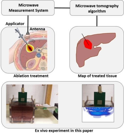
1. Introduction
2. Materials and Methods
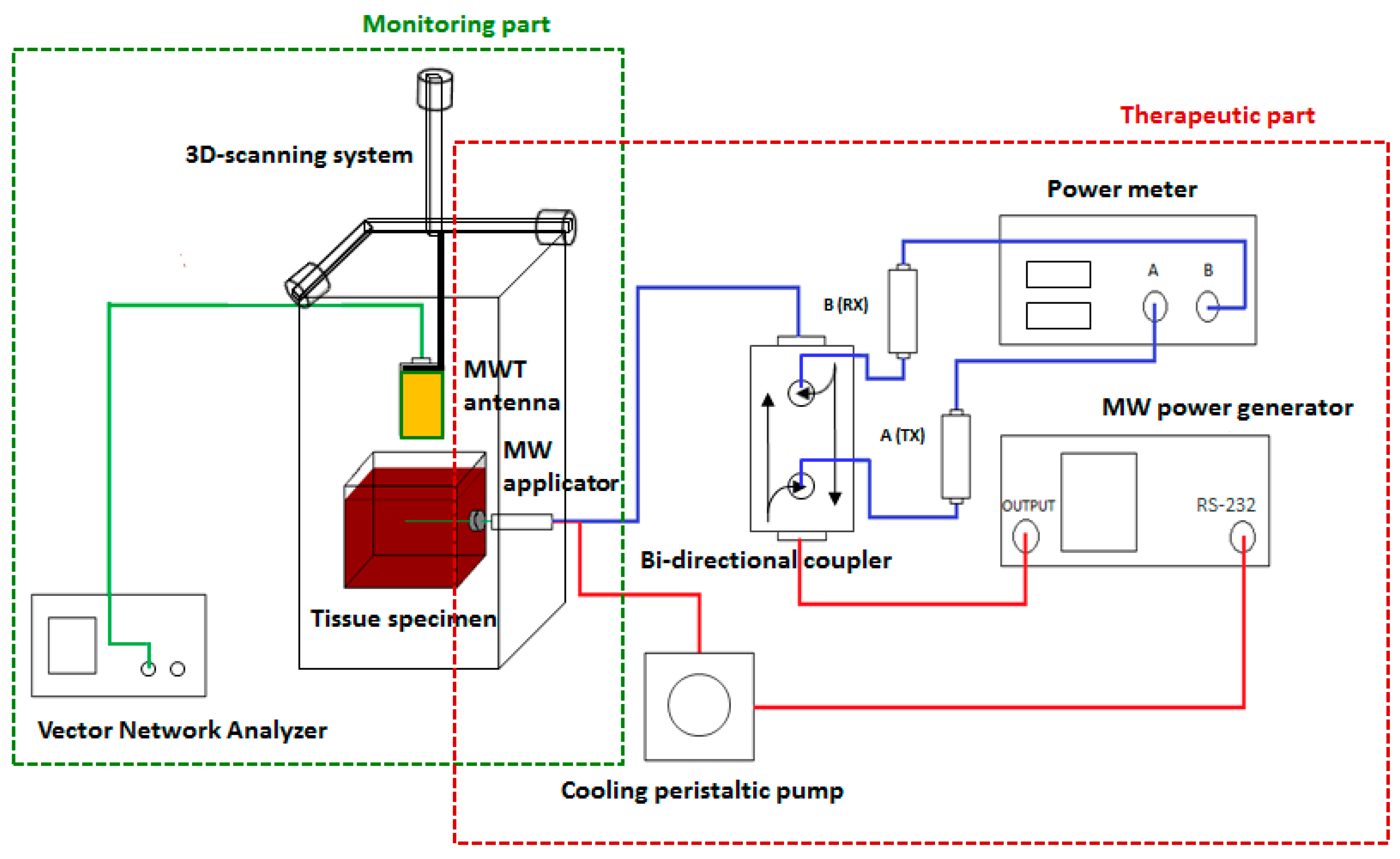
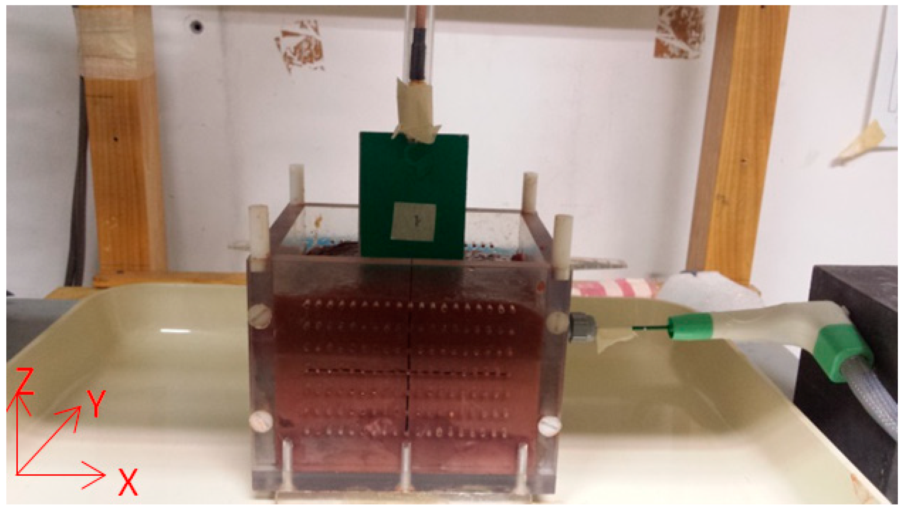
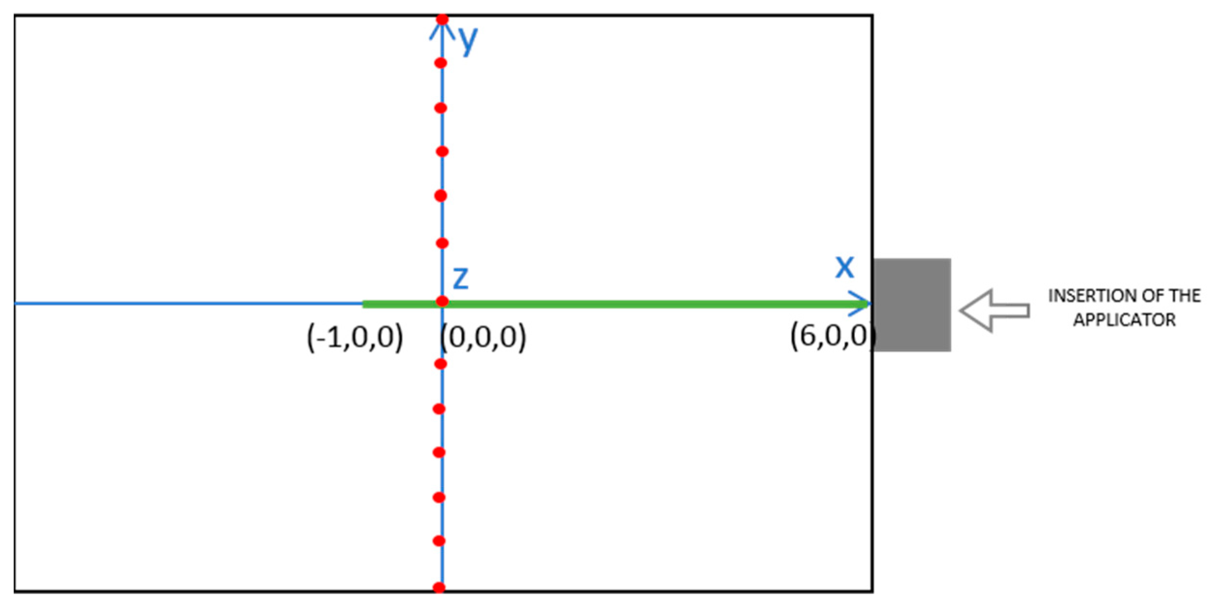
2.1. Experimental Set-Up
2.2. MTA Experiments
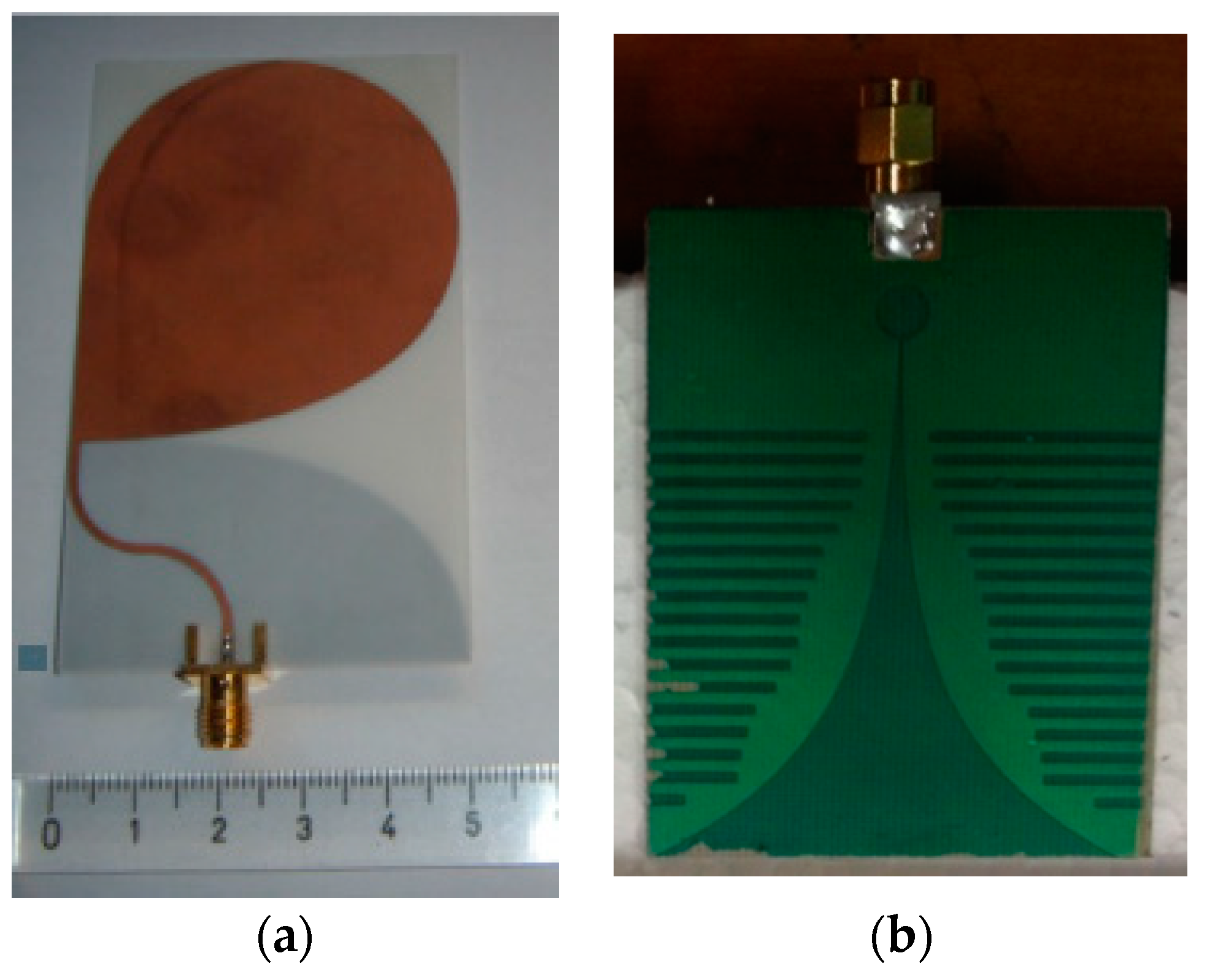
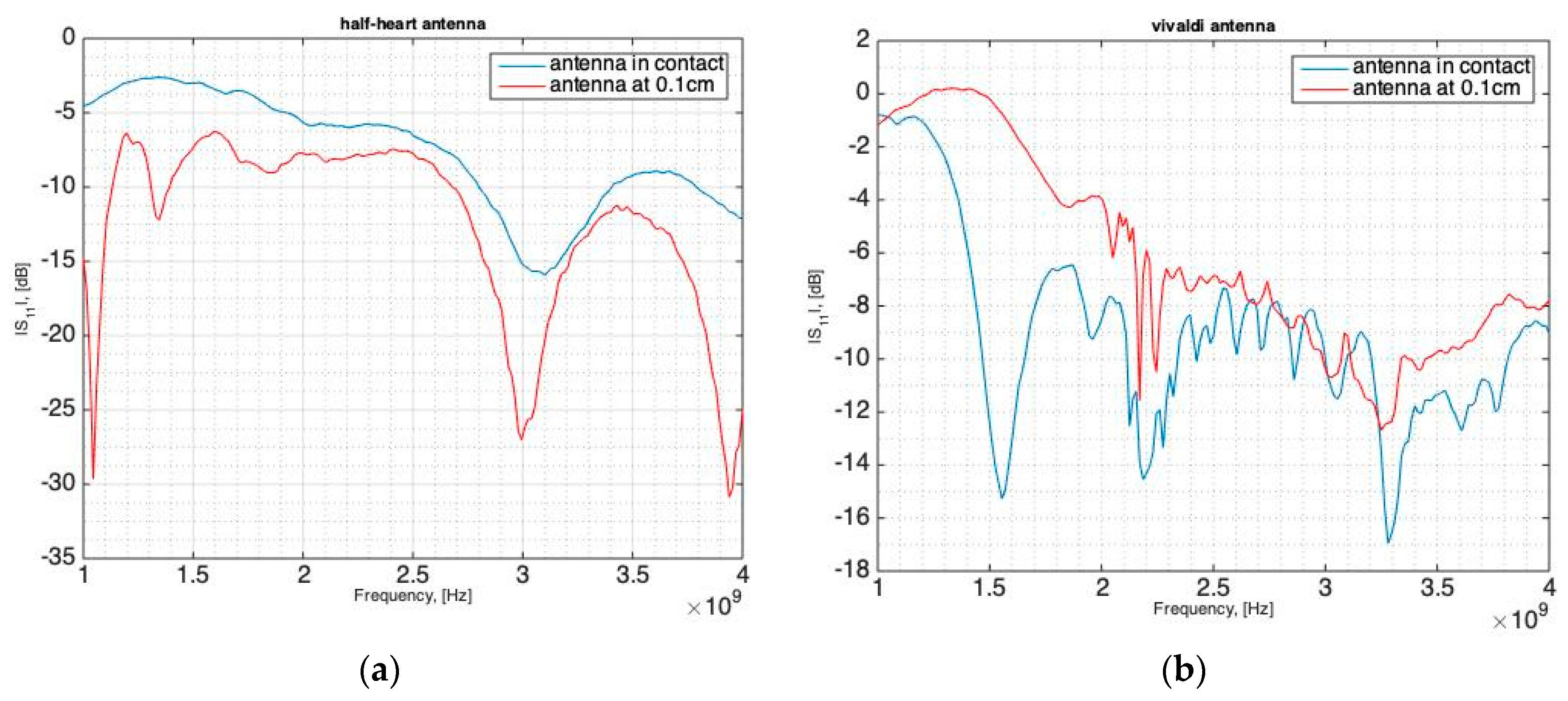
2.3. MWT Measurements
2.4. Imaging Algorithm and Assessment Criterion
2.4.1. Choice of the Regularization Parameter
2.4.2. Assessment Criterion
3. Results
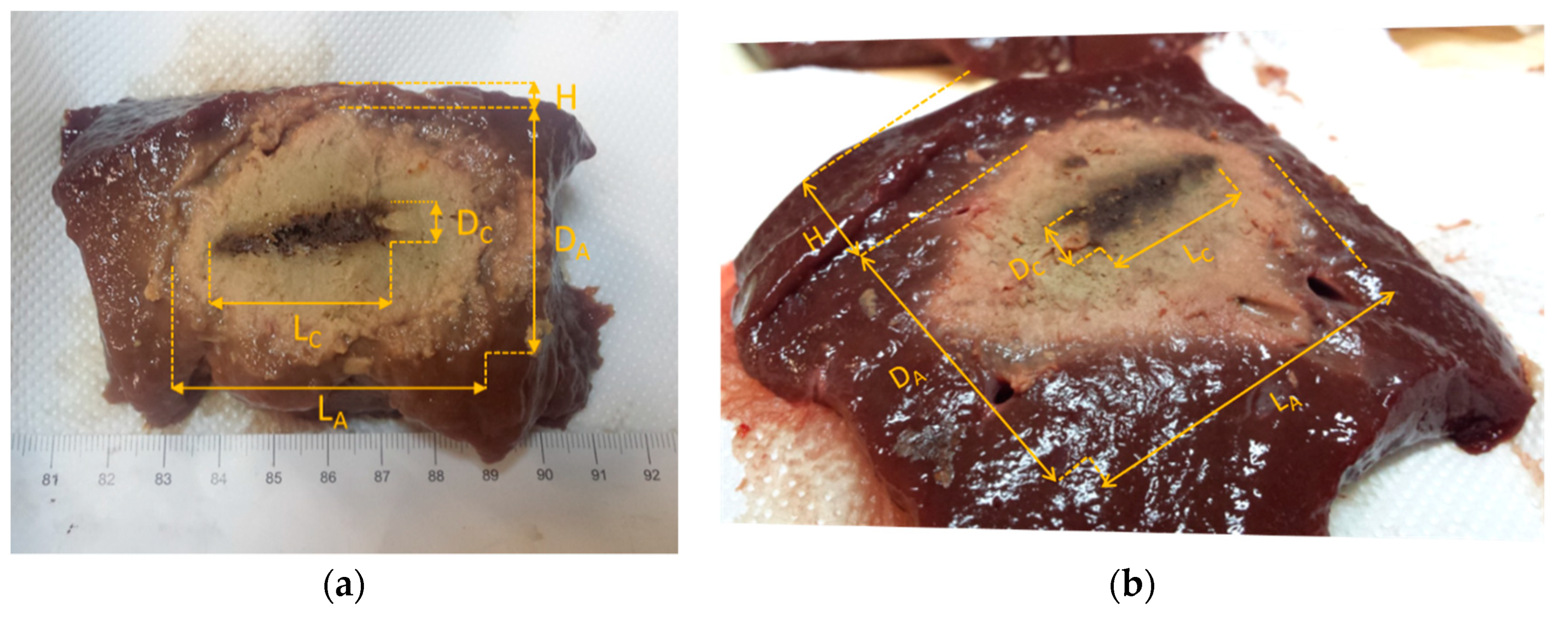
3.1. Ex Vivo Post-Ablation Analysis
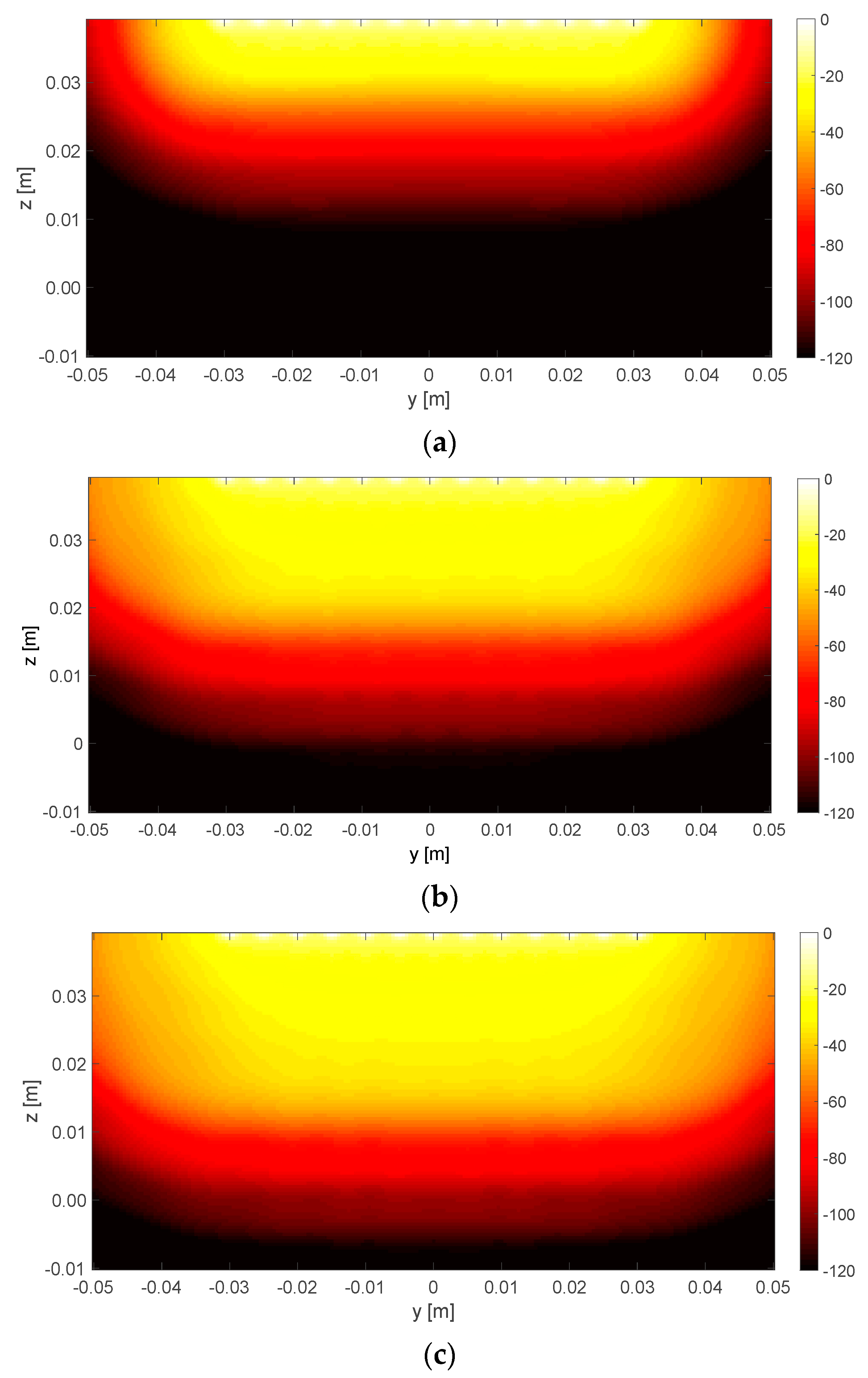
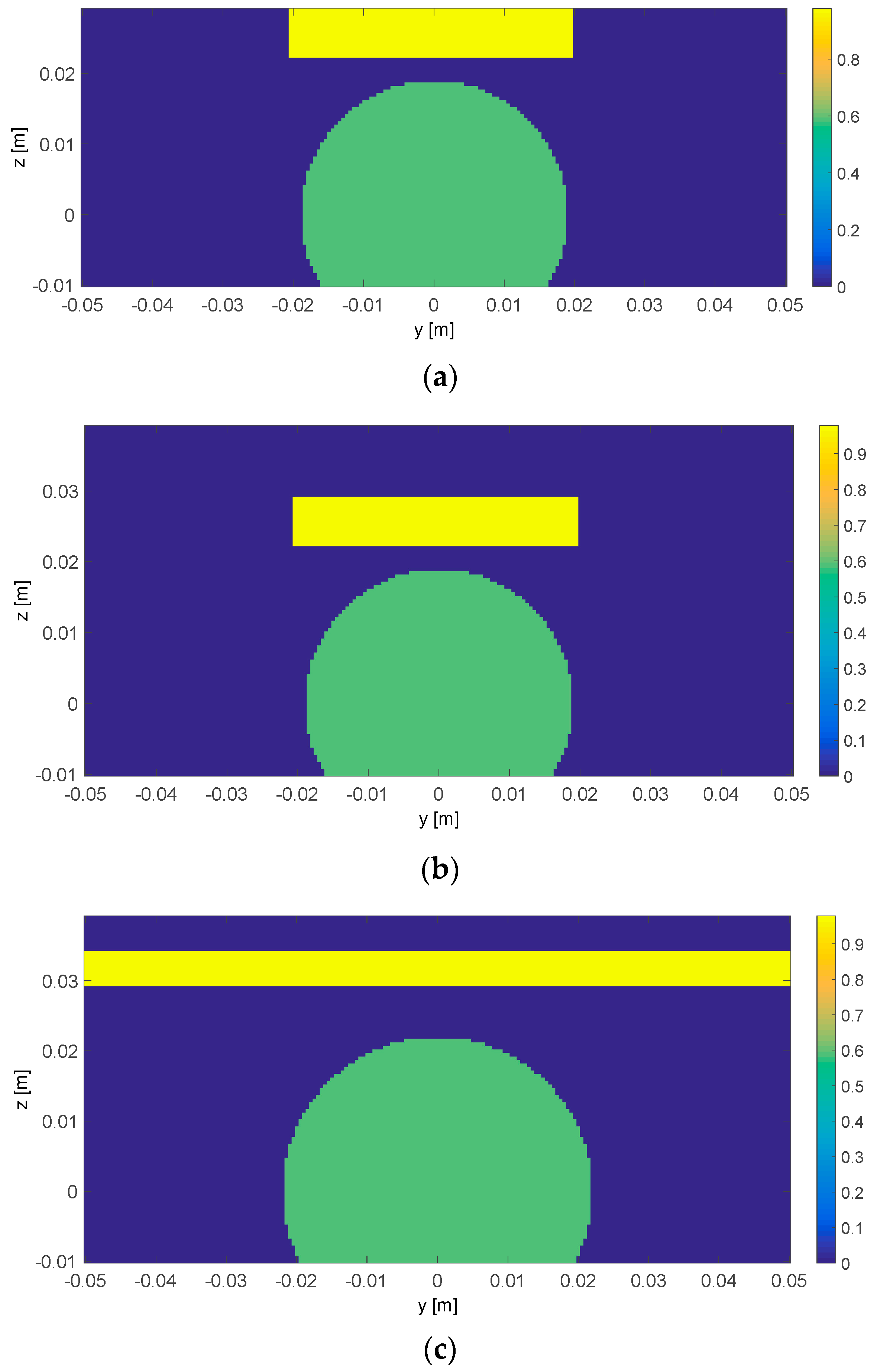
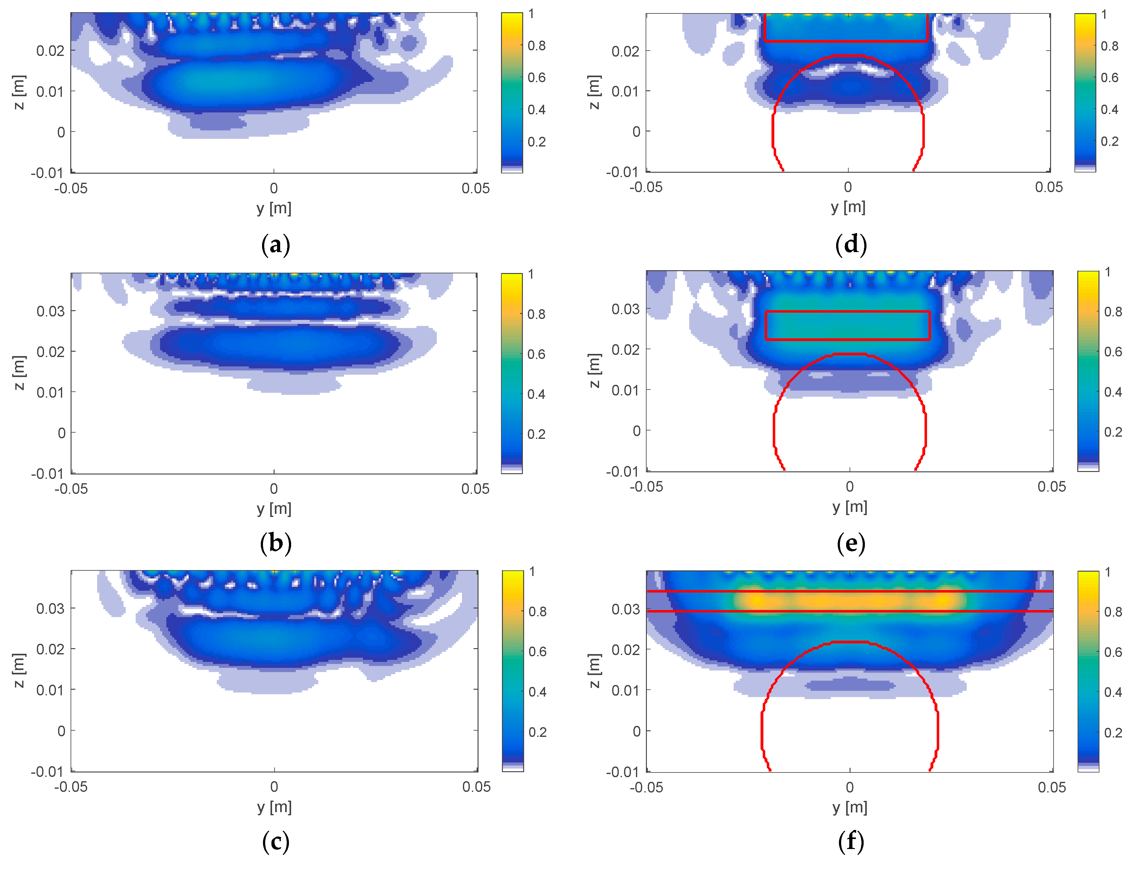
3.2. Microwave Tomography Results
4. Discussion
5. Conclusions
Author Contributions
Funding
Acknowledgments
Conflicts of Interest
Appendix A

Appendix B
References
- Goldberg, S.N.; Gazelle, G.S.; Mueller, P.R. Thermal ablation therapy for focal malignancy: A unified approach to underlying principles, techniques, and diagnostic imaging guidance. Am. J. Roentgenol. 2000, 174, 323–331. [Google Scholar] [CrossRef] [PubMed]
- Ahmed, M.; Brace, C.L.; Lee, F.T., Jr.; Goldberg, S.N. Principles of and advances in percutaneous ablation. Radiology 2011, 258, 351–369. [Google Scholar] [CrossRef] [PubMed]
- Skinner, M.G.; Lizukay, M.N.; Koliosz, M.C.; Sherary, M.D. A theoretical comparison of energy sources—Microwave, ultrasound and laser—For interstitial thermal therapy. Phys. Med. Biol. 1998, 43, 3535–3547. [Google Scholar] [CrossRef]
- Meloni, M.F.; Galimberti, S.; Dietrich, C.F.; Lazzaroni, S.; Goldberg, S.N.; Abate, A.; Sironi, S.; Andreano, A. Microwave ablation of hepatic tumors with a third generation system: Locoregional efficacy in a prospective cohort study with intermediate term follow-up. Z Gastroenterol. 2016, 54, 541–547. [Google Scholar] [CrossRef] [PubMed]
- Ierardi, A.M.; Mangano, A.; Floridi, C.; Dionigi, G.; Biondi, A.; Duka, E.; Lucchina, N.; Lianos, G.D.; Carrafiello, G. A new system of microwave ablation at 2450 MHz: Preliminary experience. Updates Surg. 2015, 67, 39–45. [Google Scholar] [CrossRef] [PubMed]
- Haemmerich, D.; Laeseke, P.F. Thermal tumour ablation: Devices, clinical applications and future directions. Int. J. Hyperth. 2005, 21, 755–760. [Google Scholar] [CrossRef] [PubMed]
- Livraghi, T.; Meloni, F.; Solbiati, L.; Zanus, G. Complications of microwave ablation for liver tumors: Results of a multicenter study. Cardiovasc. Intervent. Radiol. 2012, 35, 868–874. [Google Scholar] [CrossRef] [PubMed]
- Li, M.; Yu, X.; Liang, P.; Liu, F.; Dong, B.; Zhou, P. Percutaneous microwave ablation for liver cancer adjacent to the diaphragm. Int. J. Hyperth. 2012, 28, 218–226. [Google Scholar] [CrossRef] [PubMed]
- Callstrom, M.R.; Charboneau, J.W. Technologies for ablation of hepatocellular carcinoma. Gastroenterology 2008, 134, 1831–1835. [Google Scholar] [CrossRef] [PubMed]
- Jones, C.; Badger, S.A.; Ellis, G. The role of microwave ablation in the management of hepatic colorectal metastases. Surgeon 2011, 9, 33–37. [Google Scholar] [CrossRef]
- Hoffmann, R.; Rempp, H.; Erhard, L.; Blumenstock, G.; Pereira, P.L.; Claussen, C.D.; Clasen, S. Comparison of four microwave ablation devices: An experimental study in ex vivo bovine liver. Radiology 2013, 268, 89–97. [Google Scholar] [CrossRef] [PubMed]
- Brace, C.L.; Laeseke, P.F.; Sampson, L.A.; Frey, T.M.; van der Weide, D.W.; Lee, F.T., Jr. Microwave ablation with a single small-gauge triaxial antenna: In vivo porcine liver model. Radiology 2007, 242, 435–440. [Google Scholar] [CrossRef] [PubMed]
- Emprint™ Ablation System with Thermosphere™ Technology. Available online: http://www.medtronic.com/covidien/en-us/products/ablation-systems/emprint-ablation-system.html (accessed on 4 December 2018).
- Ahmed, M.; Solbiati, L.; Brace, C.L.; Breen, D.J.; Callstrom, M.R.; Charboneau, J.W.; Chen, M.H.; Choi, B.I.; De Baère, T.; Dodd, G.D., III; et al. Image-guided tumor ablation: Standardization of terminology and reporting criteria—A 10-year update. J. Vasc. Interv. Radiol. 2014, 25, 1691–1705. [Google Scholar] [CrossRef] [PubMed]
- Saccomandi, P.; Schena, E.; Silvestri, S. Techniques for temperature monitoring during laser-induced thermotherapy: An overview. Int. J. Hyperth. 2013, 29, 609–619. [Google Scholar] [CrossRef] [PubMed]
- Lopresto, V.; Pinto, R.; Farina, L.; Cavagnaro, M. Treatment planning in microwave thermal ablation: Clinical gaps and recent research advances. Int. J. Hyperth. 2017, 33, 83–100. [Google Scholar] [CrossRef]
- Garrean, S.; Hering, J.; Saied, A.; Hoopes, P.J.; Helton, W.S.; Ryan, T.P.; Espat, N.J. Ultrasound monitoring of a novel microwave ablation (MWA) device in porcine liver: Lessons learned and phenomena observed on ablative effects near major intrahepatic vessels. J. Gastrointest. Surg. 2009, 13, 334–340. [Google Scholar] [CrossRef]
- Han, Z.-Y.; Liang, P.; Yu, X.-L.; Cheng, Z.-G.; Liu, F.-Y.; Yu, J. A clinical study of thermal monitoring techniques of ultrasound-guided microwave ablation for hepatocellular carcinoma in high-risk locations. Sci. Rep. 2017, 7, 41246. [Google Scholar]
- Cazzato, R.L.; Buy, X.; Alberti, N.; Fonck, M.; Grasso, R.F.; Palussière, J. Flat-panel cone-beam CT-guided radiofrequency ablation of very small (1.5 cm) liver tumors: Technical note on a preliminary experience. Cardiovasc. Intervent. Radiol. 2015, 38, 206–212. [Google Scholar] [CrossRef]
- Pandeya, G.D.; Greuter, M.J.; de Jong, K.P.; Schmidt, B.; Flohr, T.; Oudkerk, M. Feasibility of noninvasive temperature assessment during radiofrequency liver ablation on computed tomography. J. Comput. Assist. Tomogr. 2011, 35, 356–360. [Google Scholar] [CrossRef]
- Bruners, P.; Pandeya, G.D.; Levit, E.; Roesch, E.; Penzkofer, T.; Isfort, P.; Schmidt, B.; Greuter, M.J.; Oudkerk, M.; Schmitz-Rode, T.; et al. CT-based temperature monitoring during hepatic RF ablation: Feasibility in an animal model. Int. J. Hyperth. 2012, 28, 55–61. [Google Scholar] [CrossRef]
- Fani, F.; Schena, E.; Saccomandi, P.; Silvestri, S. CT-based thermometry: An overview. Int. J. Hyperth. 2014, 30, 219–227. [Google Scholar] [CrossRef] [PubMed]
- Clasen, S.; Pereira, P.L. Magnetic resonance guidance for radiofrequency ablation of liver tumors. J. Magn. Reson. Imaging 2008, 27, 421–433. [Google Scholar] [CrossRef]
- McDannold, N. Quantitative MRI-based temperature mapping based on the proton resonant frequency shift: Review of validation studies. Int. J. Hyperth. 2005, 21, 533–546. [Google Scholar] [CrossRef] [PubMed]
- Bucci, O.M.; Cavagnaro, M.; Crocco, L.; Lopresto, V.; Scapaticci, R. Microwave ablation monitoring via microwave tomography: A numerical feasibility assessment. In Proceedings of the 2016 10th European Conference on Antennas and Propagation (EuCAP), Davos, Switzerland, 10–15 April 2016; pp. 1–5. [Google Scholar]
- Bellizzi, G.G.; Crocco, L.; Cavagnaro, M.; Farina, L.; Lopresto, V.; Scapaticci, R. A full-wave numerical assessment of microwave tomography for monitoring cancer ablation. In Proceedings of the 2017 11th European Conference on Antennas and Propagation (EUCAP), Paris, France, 19–24 March 2017; pp. 3722–3725. [Google Scholar]
- Scapaticci, R.; Bellizzi, G.G.; Cavagnaro, M.; Lopresto, V.; Crocco, L. Exploiting Microwave Imaging Methods for Real-Time Monitoring of Thermal Ablation. Int. J. Ant. Propag. 2017, 2017, 5231065. [Google Scholar] [CrossRef]
- Lopresto, V.; Pinto, R.; Lovisolo, G.A.; Cavagnaro, M. Changes in the dielectric properties of ex vivo bovine liver during microwave thermal ablation at 2.45 GHz. Phys. Med. Biol. 2012, 57, 2309–2327. [Google Scholar] [CrossRef] [PubMed]
- Lopresto, V.; Pinto, R.; Cavagnaro, M. Experimental characterisation of the thermal lesion induced by microwave ablation. Int. J. Hyperth. 2014, 30, 110–118. [Google Scholar] [CrossRef] [PubMed]
- Cavagnaro, M.; Pinto, R.; Lopresto, V. Numerical models to evaluate the temperature increase induced by ex vivo microwave thermal ablation. Phys. Med. Biol. 2015, 60, 3287–3311. [Google Scholar] [CrossRef] [PubMed]
- Chen, G.; Stang, J.; Haynes, M.; Leuthardt, E.; Moghaddam, M. Real-Time Three-Dimensional Microwave Monitoring of Interstitial Thermal Therapy. IEEE Trans. Biomed. Eng. 2018, 65, 528–538. [Google Scholar] [CrossRef]
- Cavagnaro, M.; Amabile, C.; Bernardi, P.; Pisa, S.; Tosoratti, N. A minimally invasive antenna for microwave ablation therapies: Design, performances, and experimental assessment. IEEE Trans. Biomed. Eng. 2011, 58, 949–959. [Google Scholar] [CrossRef] [PubMed]
- Bur, J.A. Dielectric properties of polymers at microwave frequencies: A review. Polymer 1985, 26, 963–977. [Google Scholar] [CrossRef]
- Amabile, C.; Farina, L.; Lopresto, V.; Pinto, R.; Cassarino, S.; Tosoratti, N.; Goldberg, S.N.; Cavagnaro, M. Tissue shrinkage in microwave ablation of liver: An ex vivo predictive model. Int. J. Hyperth. 2017, 33, 101–109. [Google Scholar] [CrossRef] [PubMed]
- Lopresto, V.; Strigari, L.; Farina, L.; Minosse, S.; Pinto, R.; D’Alessio, D.; Cassano, B.; Cavagnaro, M. CT-based investigation of the contraction of ex vivo tissue undergoing microwave thermal ablation. Phys. Med. Biol. 2018, 63, 055019. [Google Scholar] [CrossRef]
- Pittella, E.; Bernardi, P.; Cavagnaro, M.; Pisa, S.; Piuzzi, E. Design of UWB antennas to monitor cardiac activity. ACES J. 2011, 26, 267–274. [Google Scholar]
- Abbak, M.; Akıncı, M.N.; Çayören, M.; Akduman, İ. Experimental Microwave Imaging with a Novel Corrugated Vivaldi Antenna. IEEE Trans. Antennas Propag. 2017, 65, 3302–3307. [Google Scholar] [CrossRef]
- Bertero, M.; Boccacci, P. Introduction to Inverse Problems in Imaging; Institute of Physics: Bristol, UK, 1998. [Google Scholar]


| MWT Antenna | Power (W) | LA (mm) | DA (mm) | LC (mm) | DC (mm) | H (mm) | Remarks |
|---|---|---|---|---|---|---|---|
| Vivaldi | 54.8 ± 0.8 | 56 | 38 | 36 | 8 | 4 | transverse contraction ~7 mm |
| Half-heart | 57.8 ± 1.2 | 54 | 44 | 31 | 8 | 13 | transverse expansion ~5 mm |
© 2018 by the authors. Licensee MDPI, Basel, Switzerland. This article is an open access article distributed under the terms and conditions of the Creative Commons Attribution (CC BY) license (http://creativecommons.org/licenses/by/4.0/).
Share and Cite
Scapaticci, R.; Lopresto, V.; Pinto, R.; Cavagnaro, M.; Crocco, L. Monitoring Thermal Ablation via Microwave Tomography: An Ex Vivo Experimental Assessment. Diagnostics 2018, 8, 81. https://doi.org/10.3390/diagnostics8040081
Scapaticci R, Lopresto V, Pinto R, Cavagnaro M, Crocco L. Monitoring Thermal Ablation via Microwave Tomography: An Ex Vivo Experimental Assessment. Diagnostics. 2018; 8(4):81. https://doi.org/10.3390/diagnostics8040081
Chicago/Turabian StyleScapaticci, Rosa, Vanni Lopresto, Rosanna Pinto, Marta Cavagnaro, and Lorenzo Crocco. 2018. "Monitoring Thermal Ablation via Microwave Tomography: An Ex Vivo Experimental Assessment" Diagnostics 8, no. 4: 81. https://doi.org/10.3390/diagnostics8040081
APA StyleScapaticci, R., Lopresto, V., Pinto, R., Cavagnaro, M., & Crocco, L. (2018). Monitoring Thermal Ablation via Microwave Tomography: An Ex Vivo Experimental Assessment. Diagnostics, 8(4), 81. https://doi.org/10.3390/diagnostics8040081