
Enhanced Superpixel-Guided ResNet Framework with Optimized Deep-Weighted Averaging-Based Feature Fusion for Lung Cancer Detection in Histopathological Images


Abstract
1. Introduction
Contribution of the Work
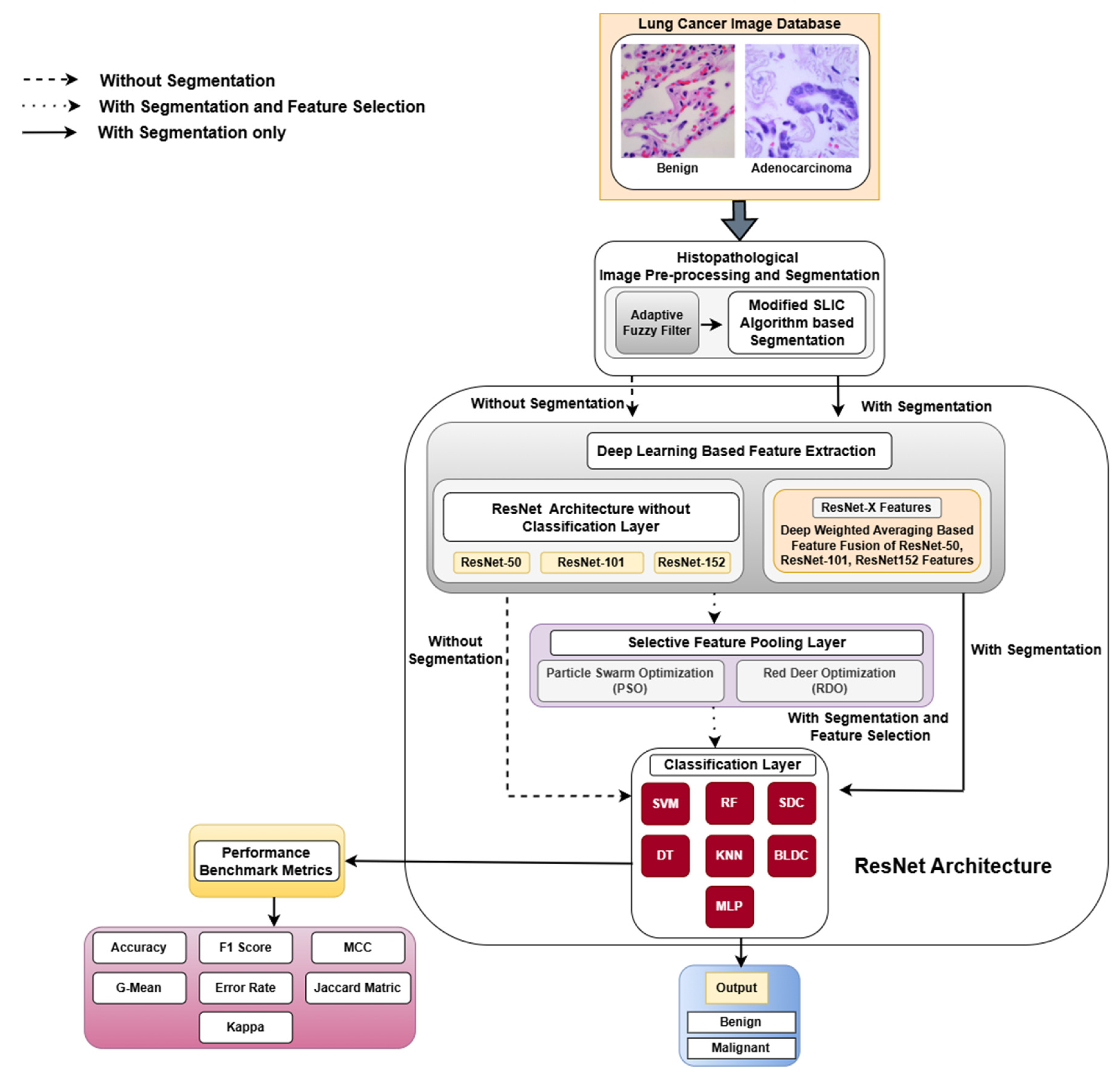
- Histopathological images are preprocessed using an adaptive fuzzy filter and segmented using the modified SLIC algorithm.
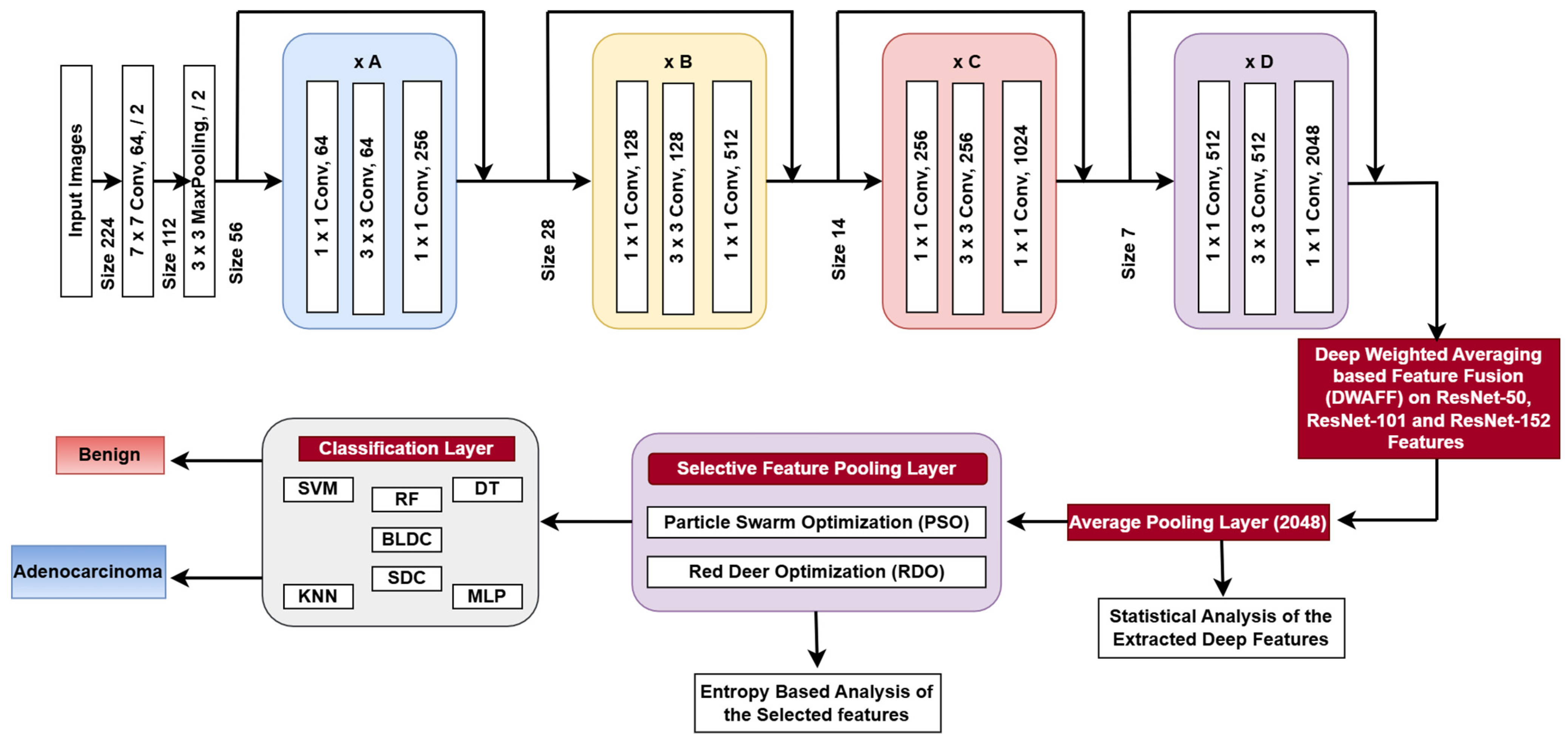
- The segmented images are passed through deep learning models such as ResNet-50, ResNet-101, and ResNet-152 for feature extraction, followed by a proposed deep-weighted averaging feature fusion technique to generate RN-X features.
- The extracted features from the ResNet models and RN-X are put into a selective feature pooling layer, which leverages PSO and RDO optimization algorithms for feature selection.
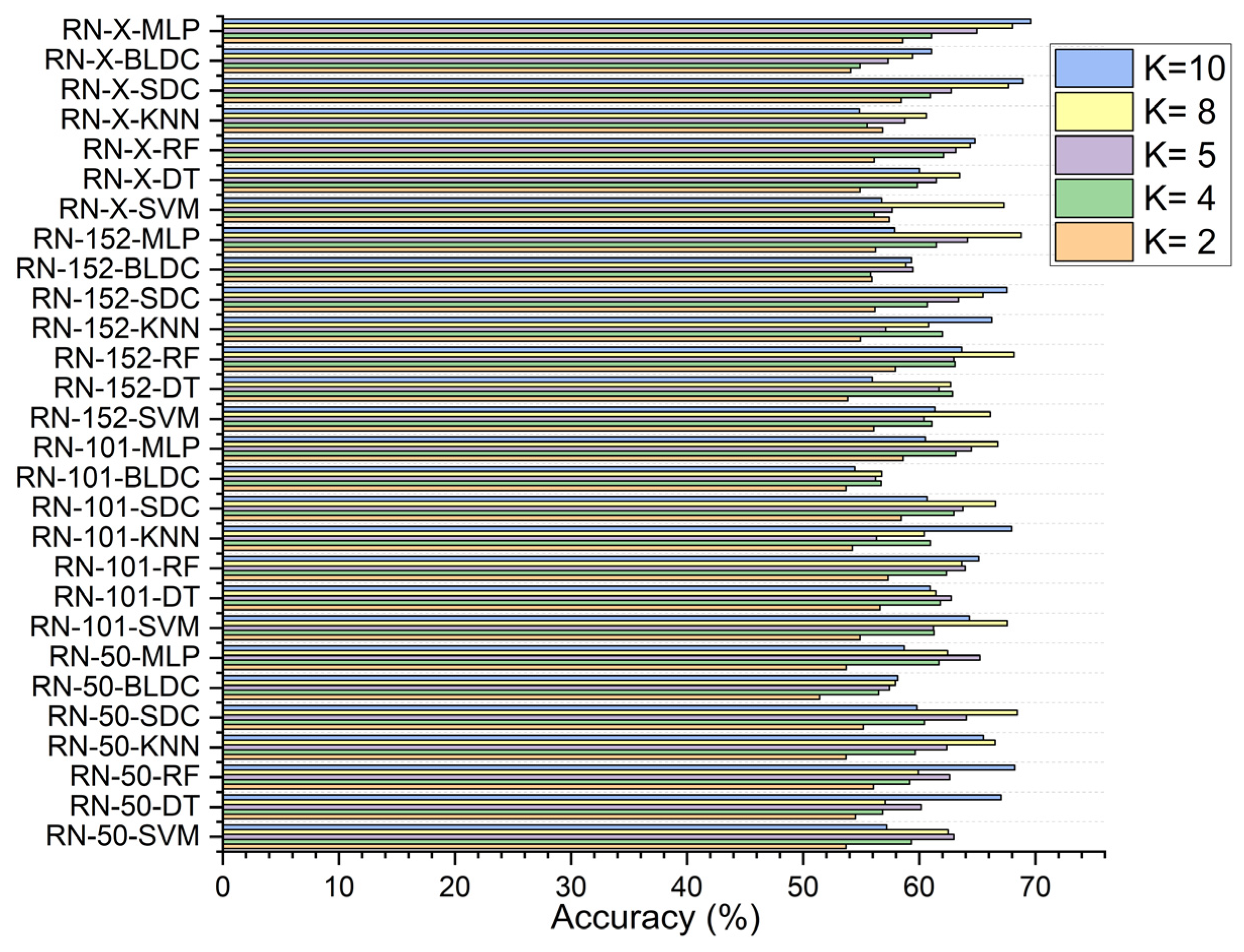
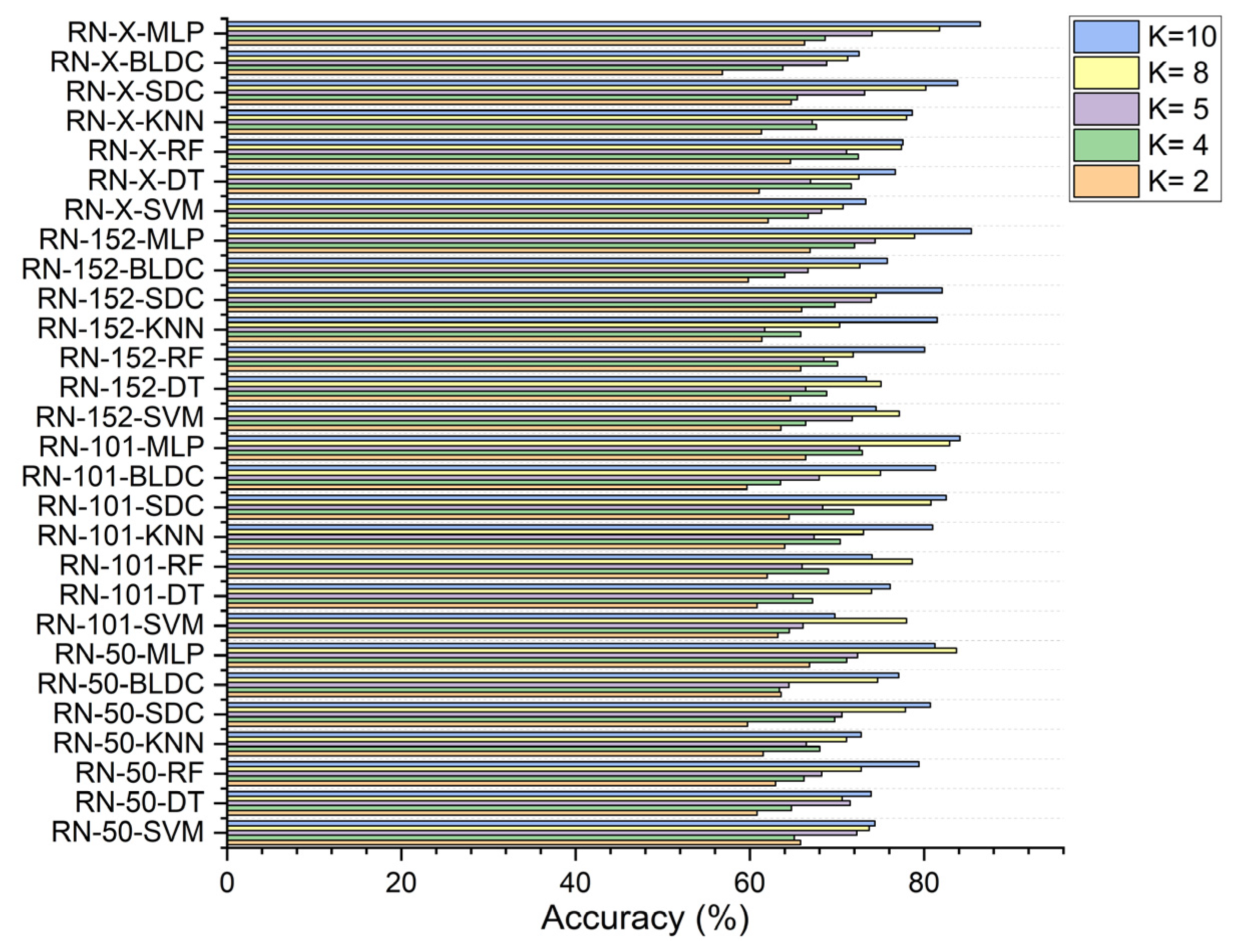
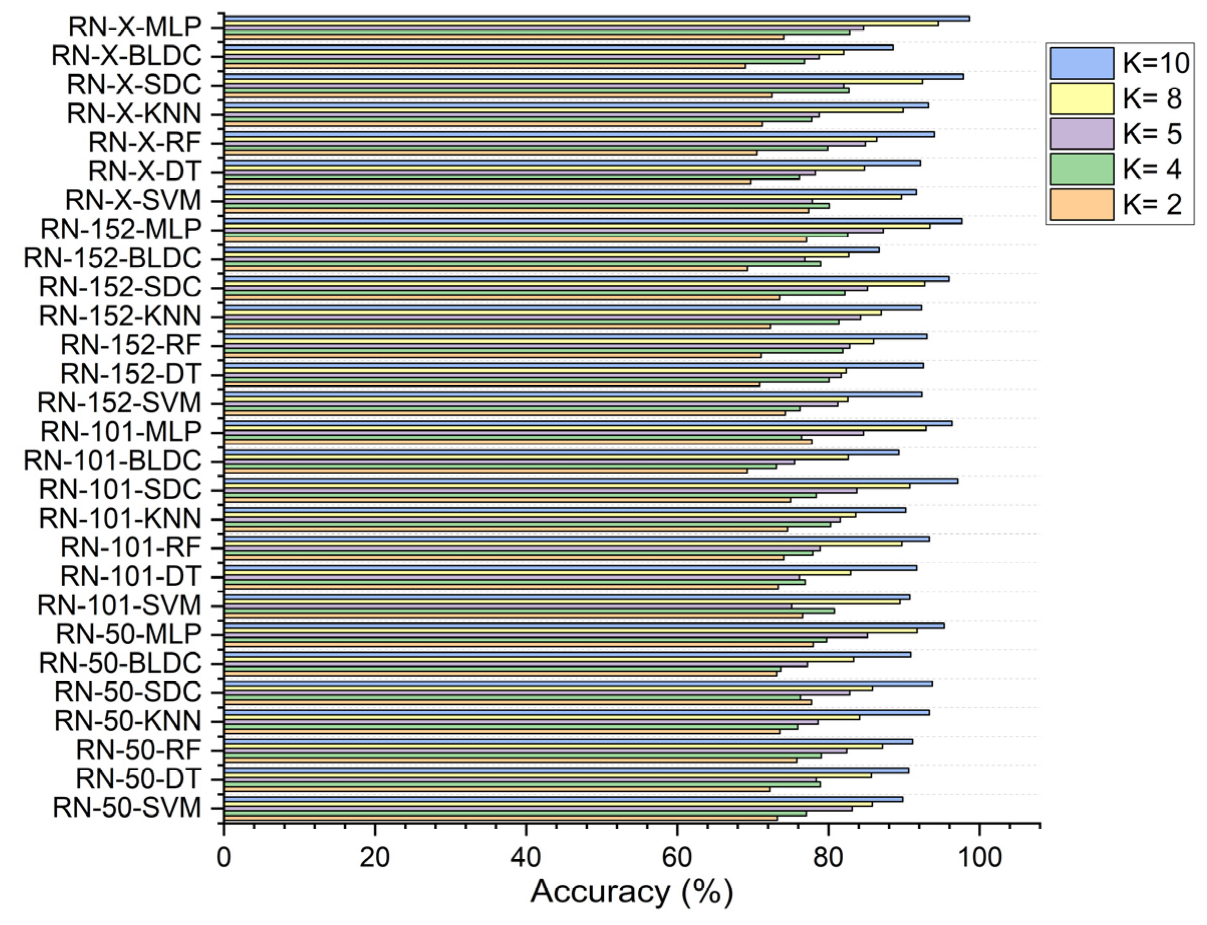
- Finally, the classification layer implements the classifiers such as SVM, DT, RF, KNN, SDC, BLDC, and MLP, evaluated using K-fold cross-validation with K values of 2, 4, 5, 8, and 10.
2. Review of Lung Cancer Detection
3. Materials and Methods
3.1. Dataset Used
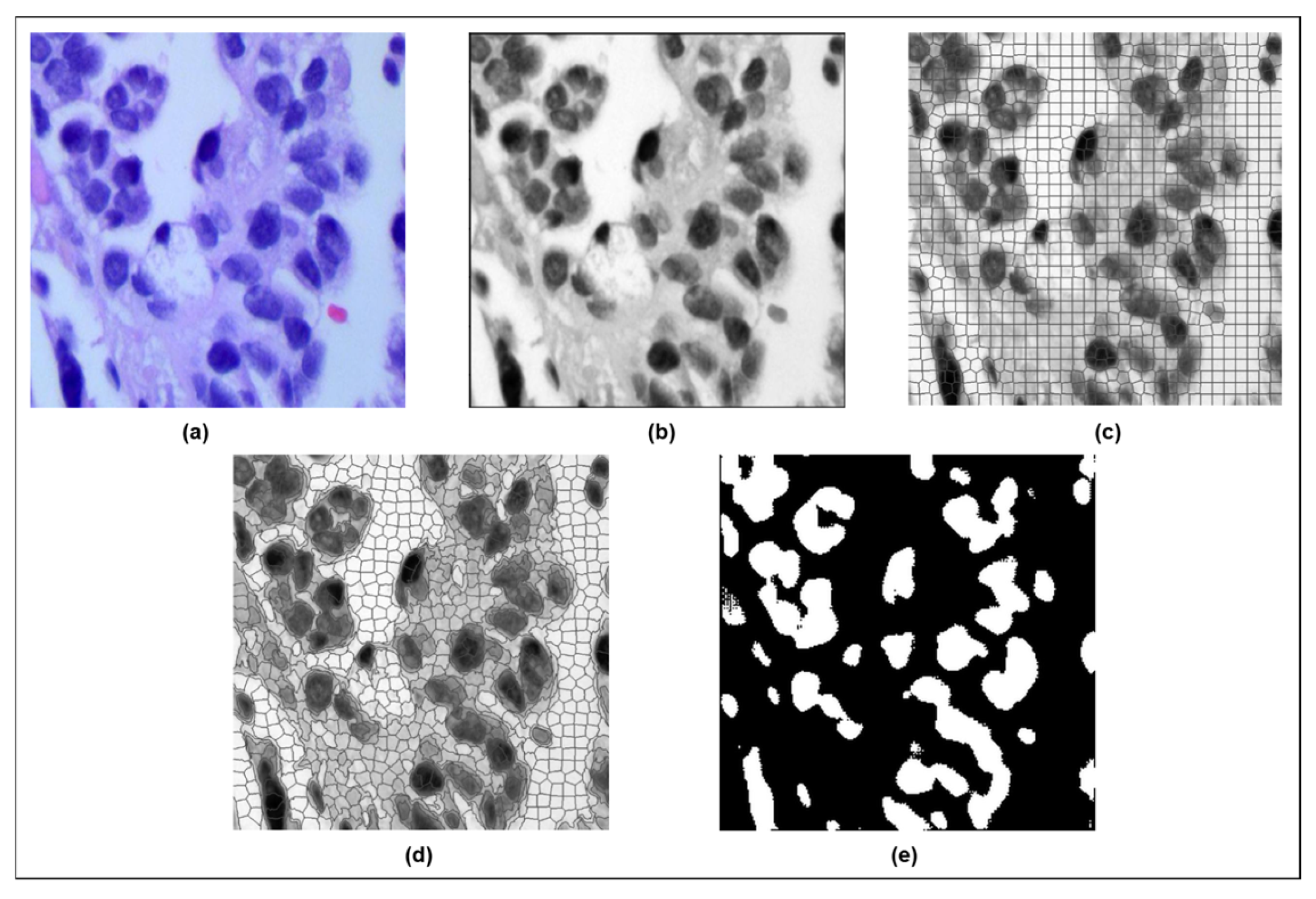
3.2. Image Preprocessing
3.3. Modified SLIC Algorithm-Based Segmentation
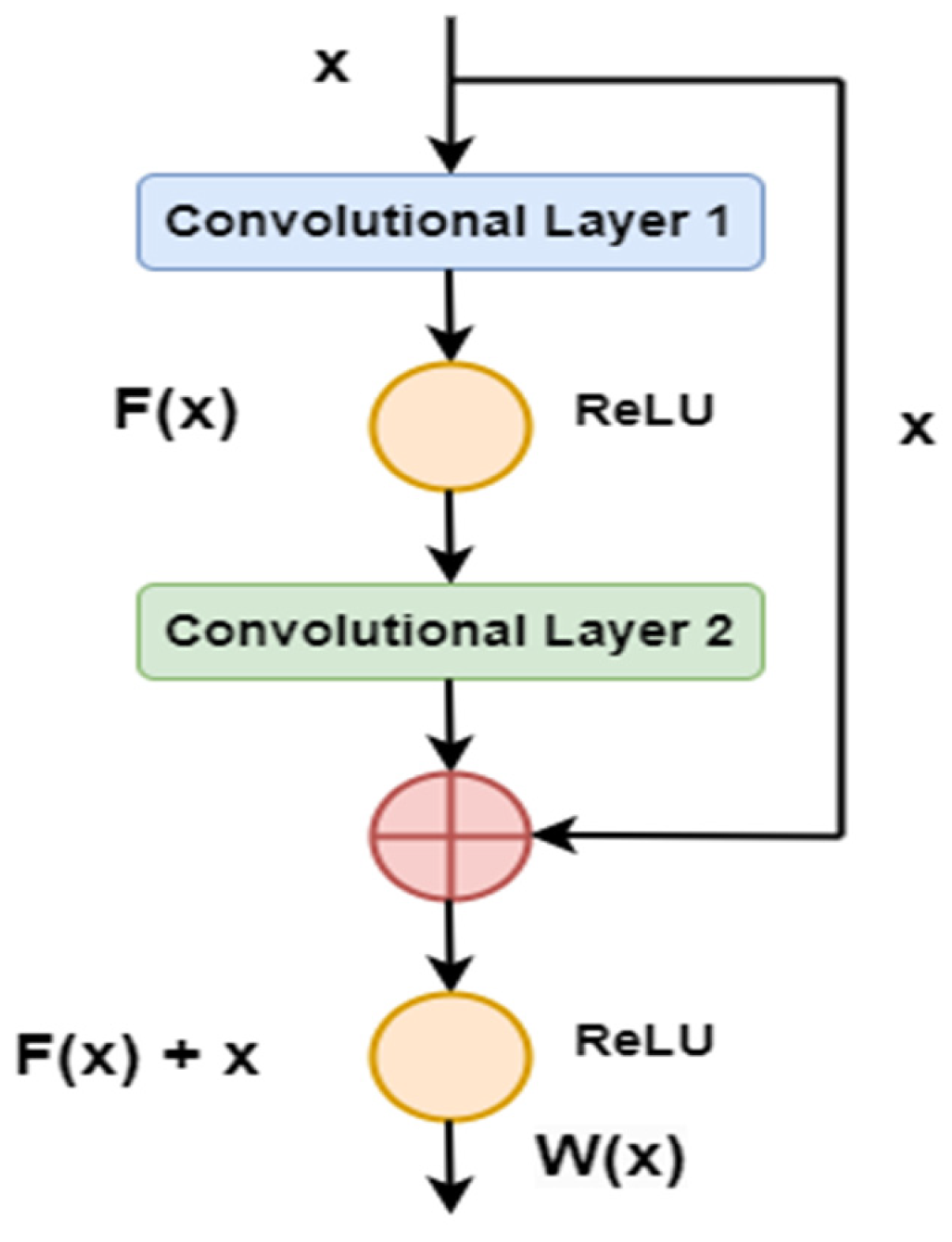
4. Deep Learning Architecture
4.1. Proposed DWAFF Technique for ResNet-X Features
| Algorithm 1. DWAFF Based Feature Fusion for ResNet-X Features | ||
| Step | Description | Details |
| Step 01 | Extract Features | Extract feature vectors for each image from ResNet-50, ResNet-101, and ResNet-152. Store the feature vectors: ResNet-50_feature [i, j], ResNet-101_feature [i, j], and ResNet-152_feature [i, j], where and . Perform K-fold Cross-Validation (K values are 2, 4, 5, 8, 10). Train the classifiers on the dataset set split. Evaluate performance of the classifiers for the different values of K using performance metrics. |
| Step 02 | Set Initial Weight Range | Initialize a range of possible weights, , and , based on the trial-and-error method, such that their sum must be equal to 1, based on the results obtained from K-fold cross-validation. |
| Step 03 | Identify Optimal Weights | For each weight combination, calculate the average performance across the K-folds. Select the weight combination that achieves the highest average performance. Optimal weights are identified as, 0.45 for ResNet-152 (), 0.35 for ResNet-101 (), and 0.20 for ResNet-50 (). |
| Step 04 | Compute Mean Values | Compute and , across all three ResNet variants. |
| Step 05 | Fuse Features for Final Feature Set | For normal cases (): fuse features of normal cases using Equation (12). For abnormal cases (): fuse features of abnormal cases using Equation (13). |
| Step 06 | Output Final Fused Features | The final fused feature set for both normal and abnormal cases, which are ResNet-X features, are used for subsequent classification tasks. |
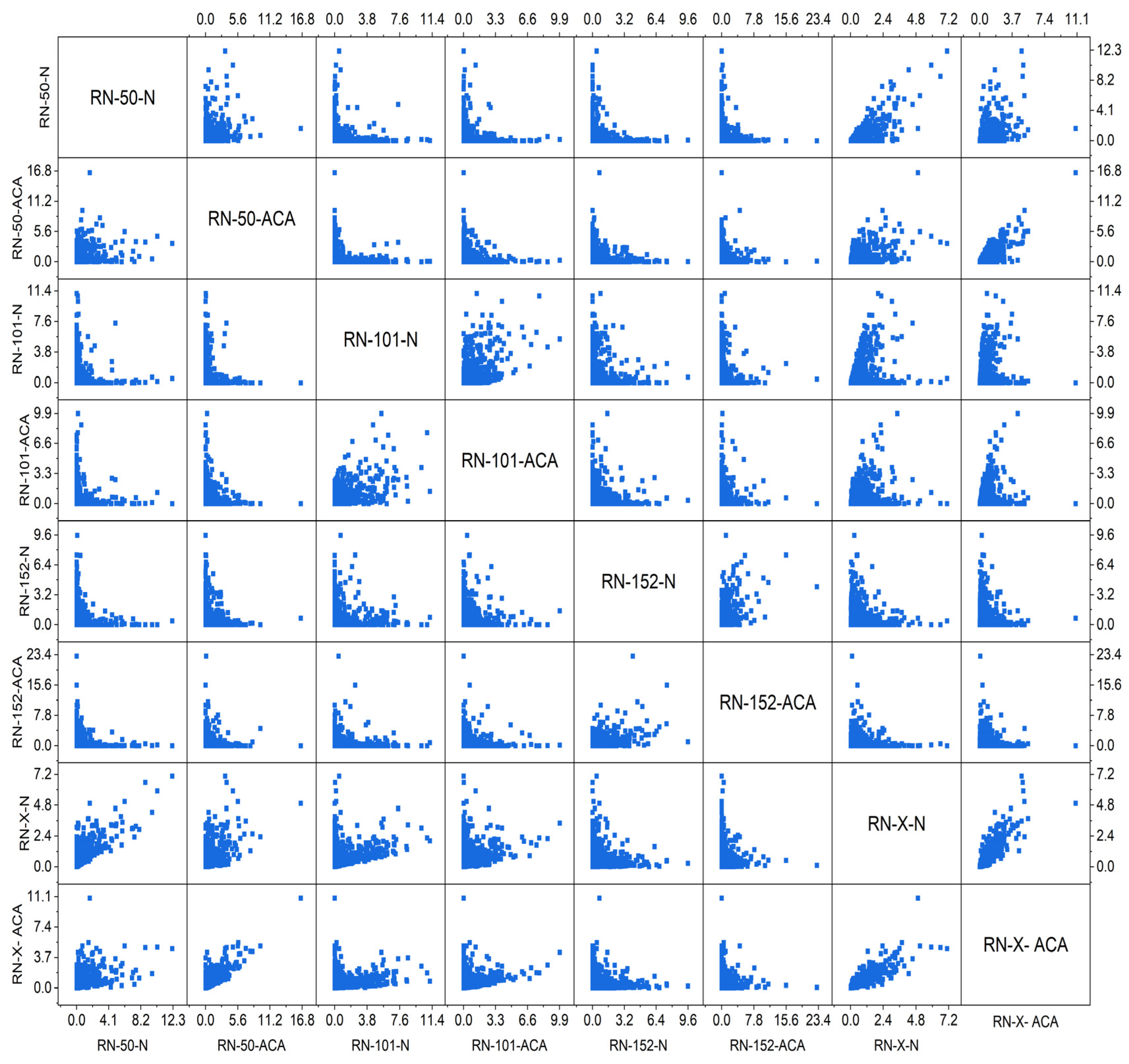
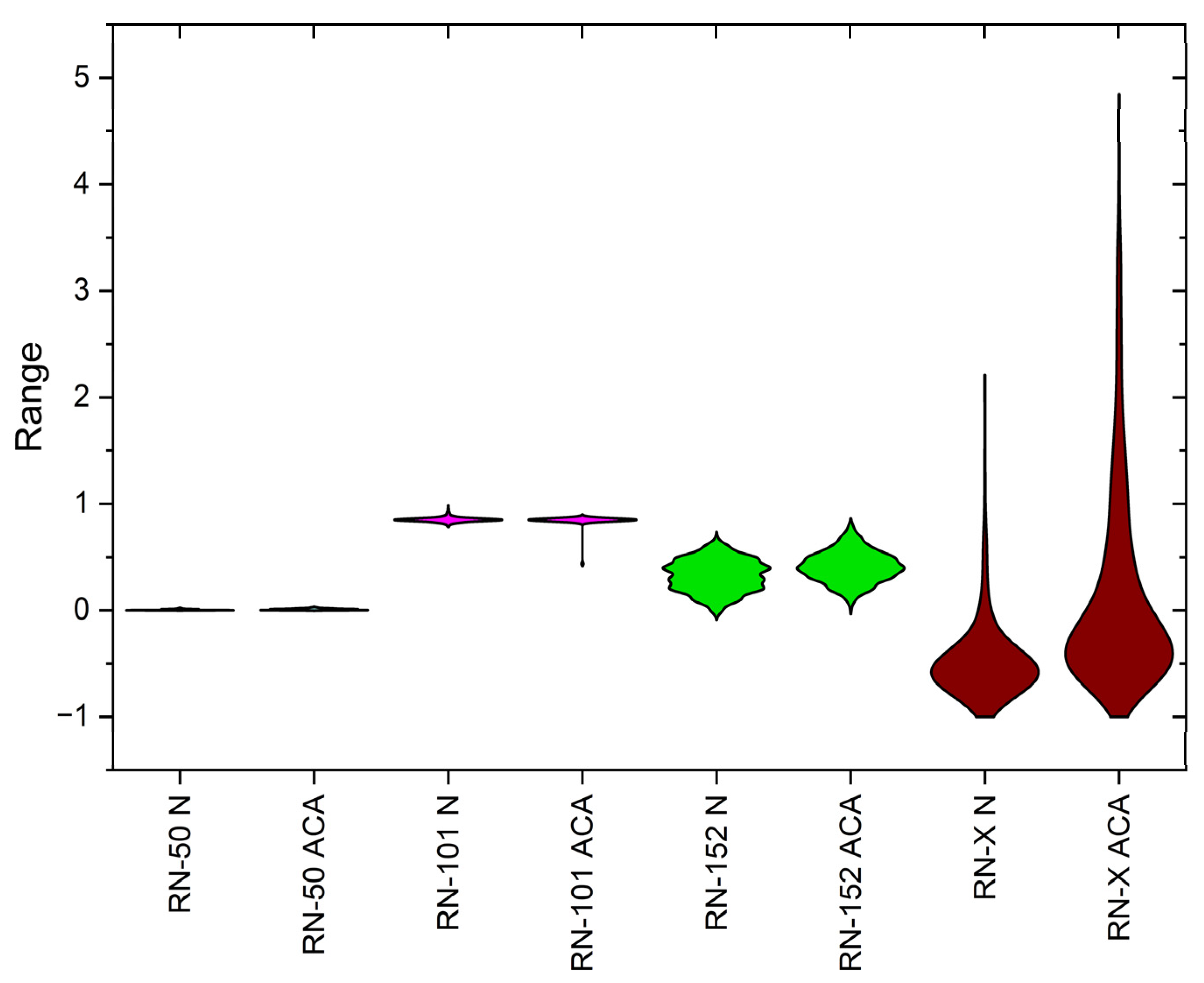
Statistical Analysis
4.2. Selective Feature Pooling Layer
4.2.1. Particle Swarm Optimization (PSO)
| Algorithm 2. Particle Swarm Optimization (PSO) as a Feature Selection | |||
| Step | Description | Details | |
| Step 01 | Initialization | - Maximum iteration count: - Inertia weight range: (, ) - Acceleration coefficients: c1, c2 - Set the position of each particle randomly: | |
| (14) | |||
| - Set the velocity of each particle randomly: | |||
| (15) | |||
| - Initialize the best position for an individual particle as and = the best of all . | |||
| Step 02 | Iteration Loop | for k = 0 to kmax − 1 do: for i = 1 to n do: Calculate the inertia weight: | |
| (16) | |||
| Update the velocity: | |||
| (17) | |||
| Update the position: | |||
| (18) | |||
| Update if the new position surpasses the previous Update if the new surpasses the current | |||
| Step 03 | Output | Output the final as the optimal solution. | |
4.2.2. Red Deer Optimization (RDO)
| Algorithm 3. Red Deer Optimization (RDO) as a Feature Selection | |||
| Step | Description | Details | |
| Step 01 | Initial Population | - Define the solution space with dimensions: | |
| (19) | |||
| Here, represents the array size, set to 50. Each component corresponds to a vector of values for each of the 50 images, as defined by the equation below: - Initialize a random population of red deer (RDs). | |||
| Step 02 | Roaring Stage | - For each male RD: -- Calculate the new position based on fitness function (FF) value using | |
| (20) | |||
| Here, UL and LL represent the maximum and minimum boundaries of the search region, respectively. The factors a1, a2 and a3 are randomly selected from a uniform distribution between zero and one. -- Update the RD position and evaluate its fitness. -- Promote successful RDs to commander status if they show improved fitness. | |||
| Step 03 | Competition Stage | - Each commander competes with random stags: -- Compute new positions: | |
| (21) | |||
| (22) | |||
| Here and are the random numbers between 0 and 1 by uniform distribution function. -- Select the position with the best fitness function (FF) to update the commander status. | |||
| Step 04 | Harem Creation Phase | - For harems with -- A commander and several hinds based on the commander’s fitness. -- Calculate the number of hinds as: | |
| (23) | |||
| -- Stags do not participate in harems. | |||
| Step 05 | Mating Phase | - Commander Mating Within Harems: Each commander mates with a proportion () of its hinds - Commander Expansion Beyond Harems: Commanders mate with a percentage () of hinds from other harems. The parameter () ranges from 0 to 1. - Stag Mating: Stags mate with the closest hind. | |
| Step 06 | Offspring Creation | - Generate new offspring using: | |
| (24) | |||
| where is the new offspring RD, c is randomly chosen between 0 and 1. For -Stage mating, replace Com with Stag. | |||
| Step 07 | Next-Generation Solution | - Retain a percentage of the best male RDs. - Select hinds and offspring for the next generation using fitness-based methods. | |
| Step 08 | Stopping Criterion | - RDO’s stopping criteria include the following: 1. Fixed number of iterations. 2. Achievement of a quality threshold. 3. Exceeding a time limit. | |
4.2.3. Entropy-Based on Statistical Analysis
Approximate Entropy
Shannon Entropy
Fuzzy Entropy
4.3. Classification Layer
4.3.1. Support Vector Machine (SVM)
4.3.2. Decision Tree (DT)
4.3.3. Random Forest (RF)
4.3.4. K-Nearest Neighbor (KNN)
4.3.5. Softmax Discriminant Classifier (SDC)
4.3.6. Multi-Layer Perceptron (MLP)
4.3.7. BLDC
5. Results and Discussion
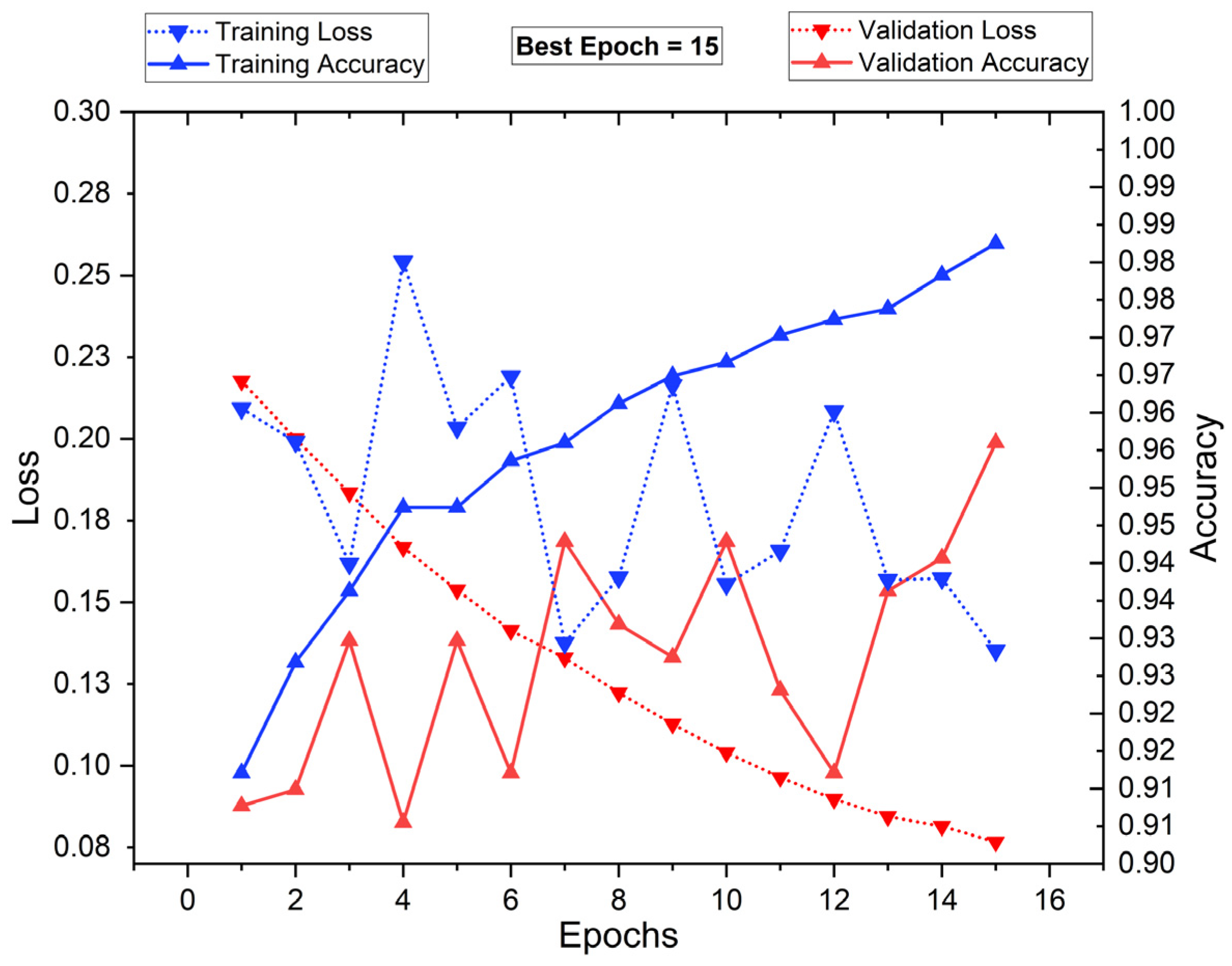
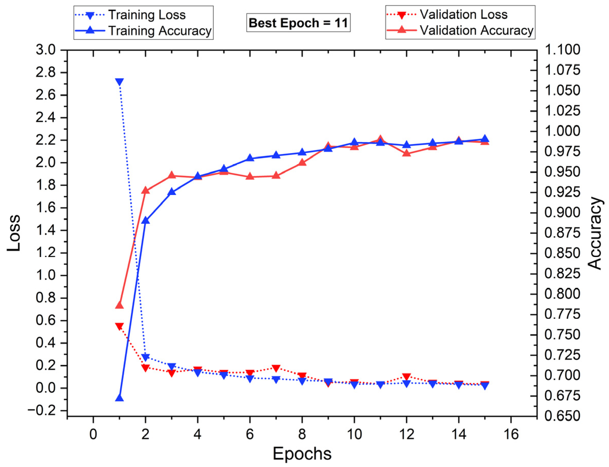
5.1. Training and Testing of the Classifiers
5.2. Standard Benchmark Metrics of the Classifiers
5.3. Performance Analysis of the Classifiers in Terms of Accuracy for Different K Values
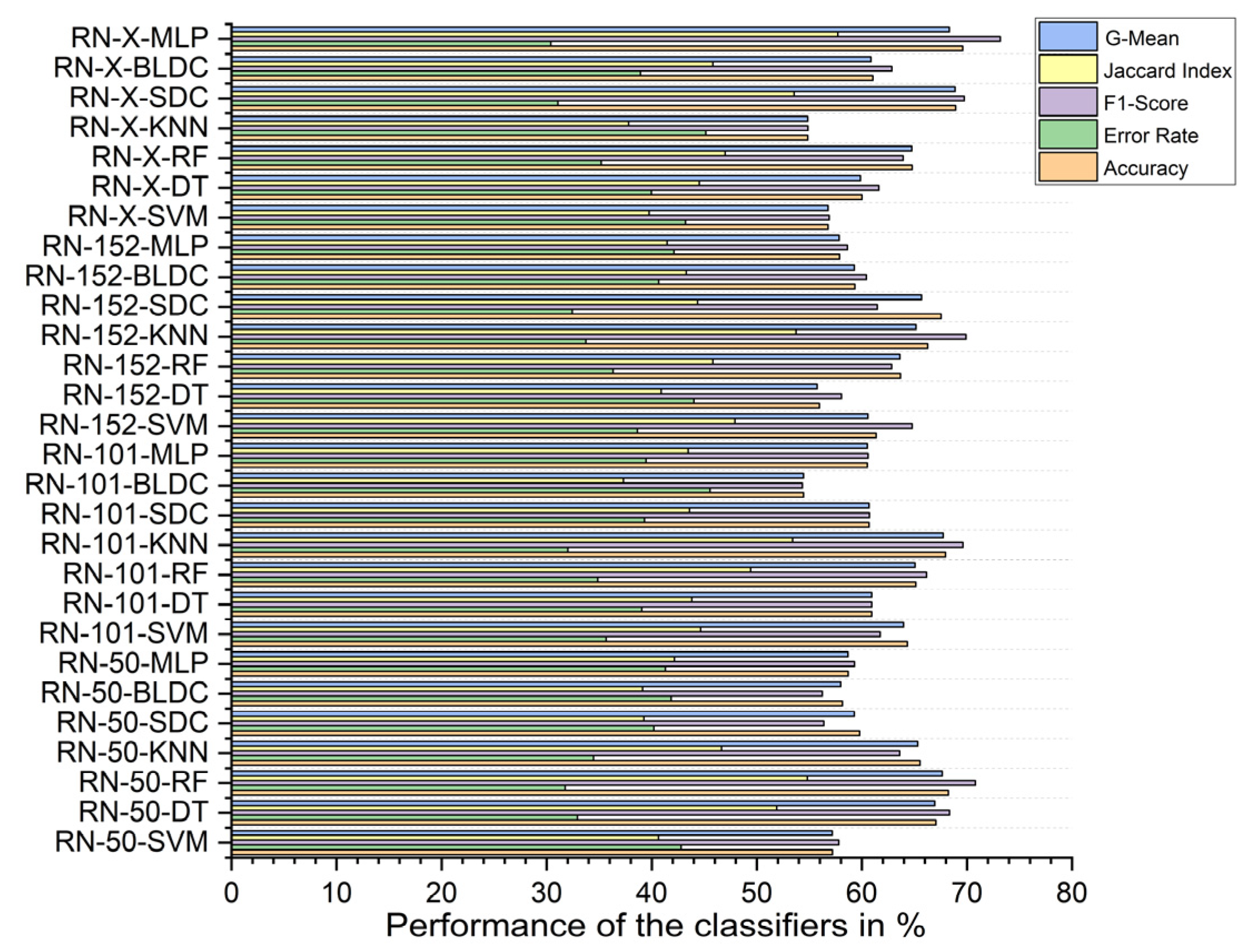
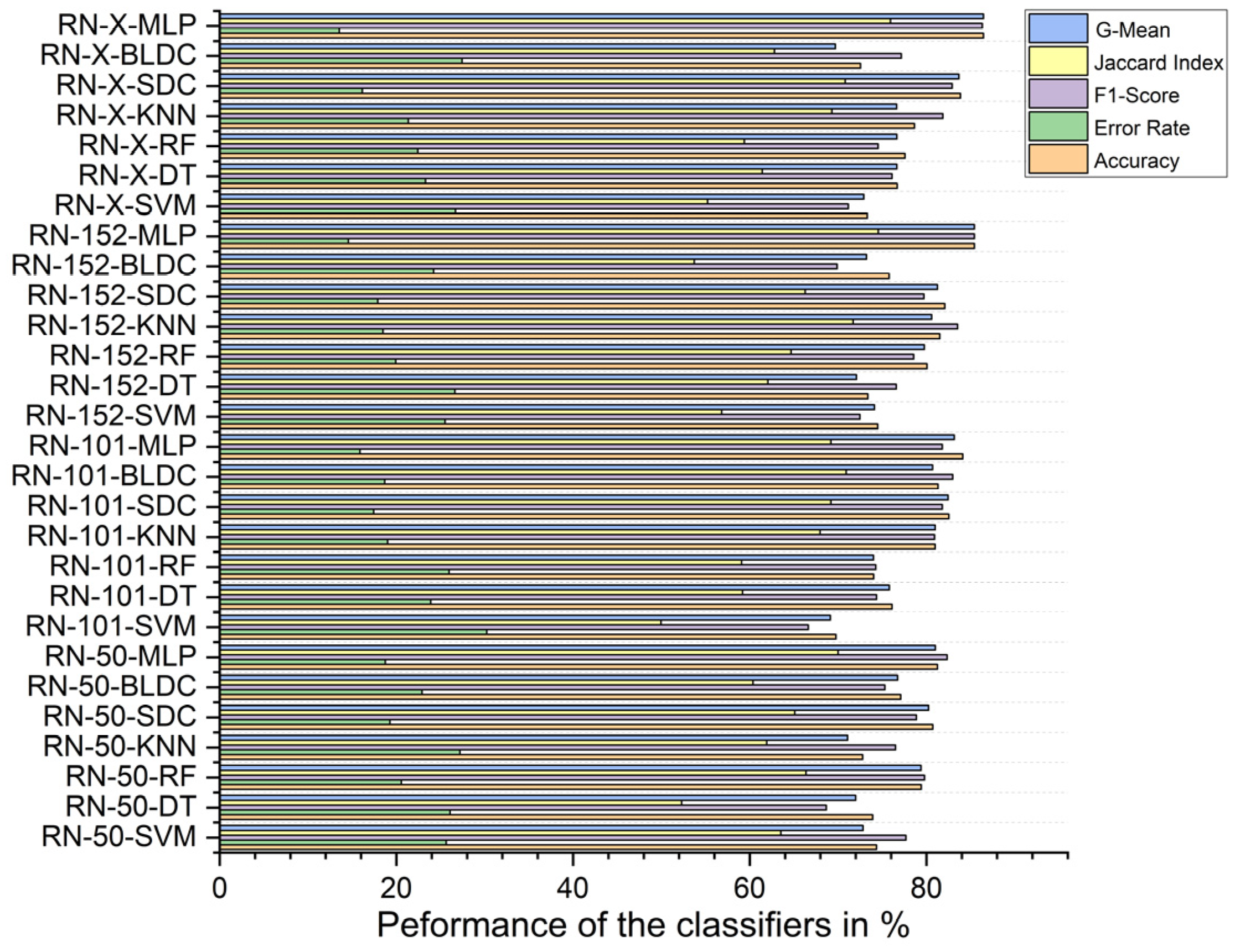
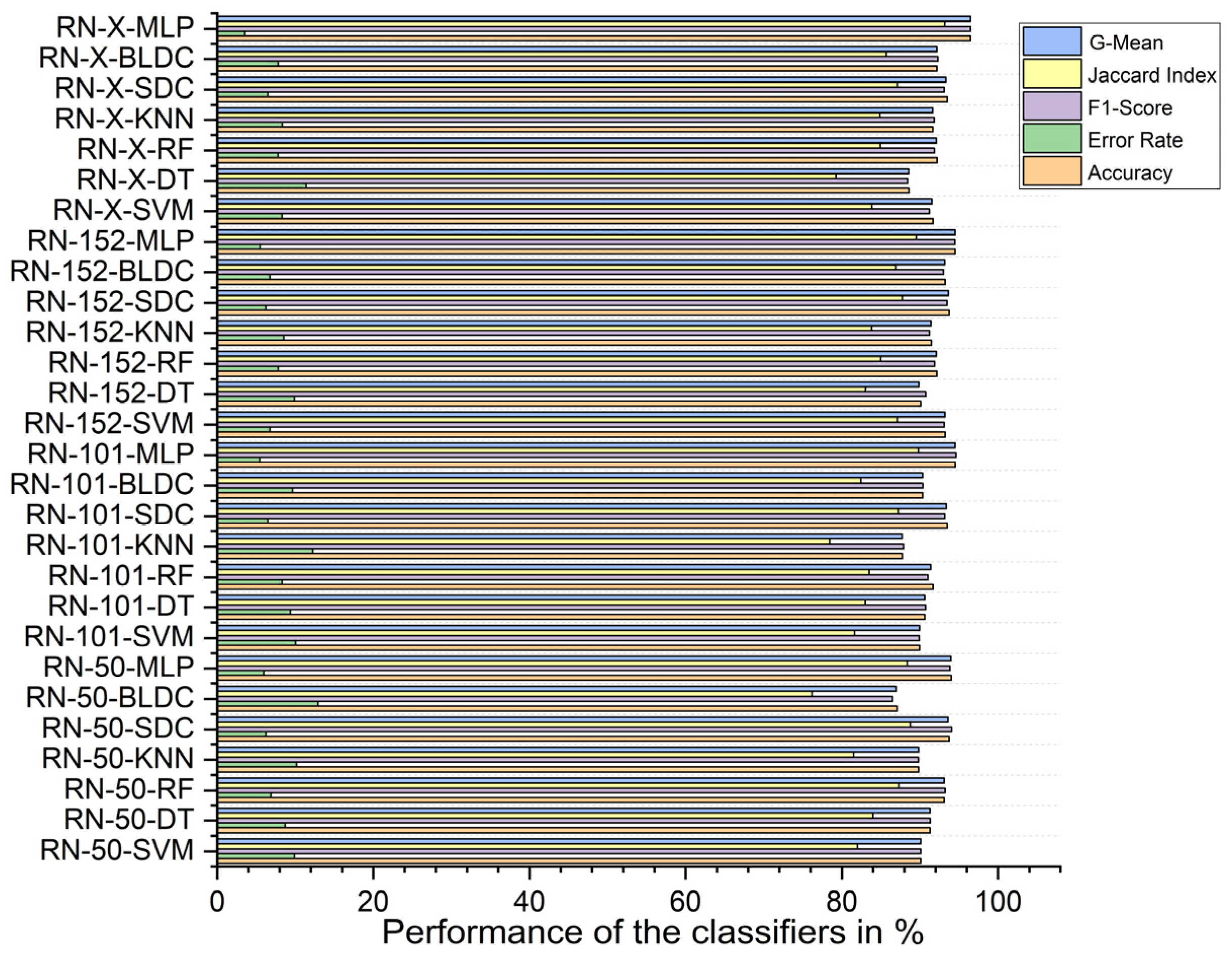
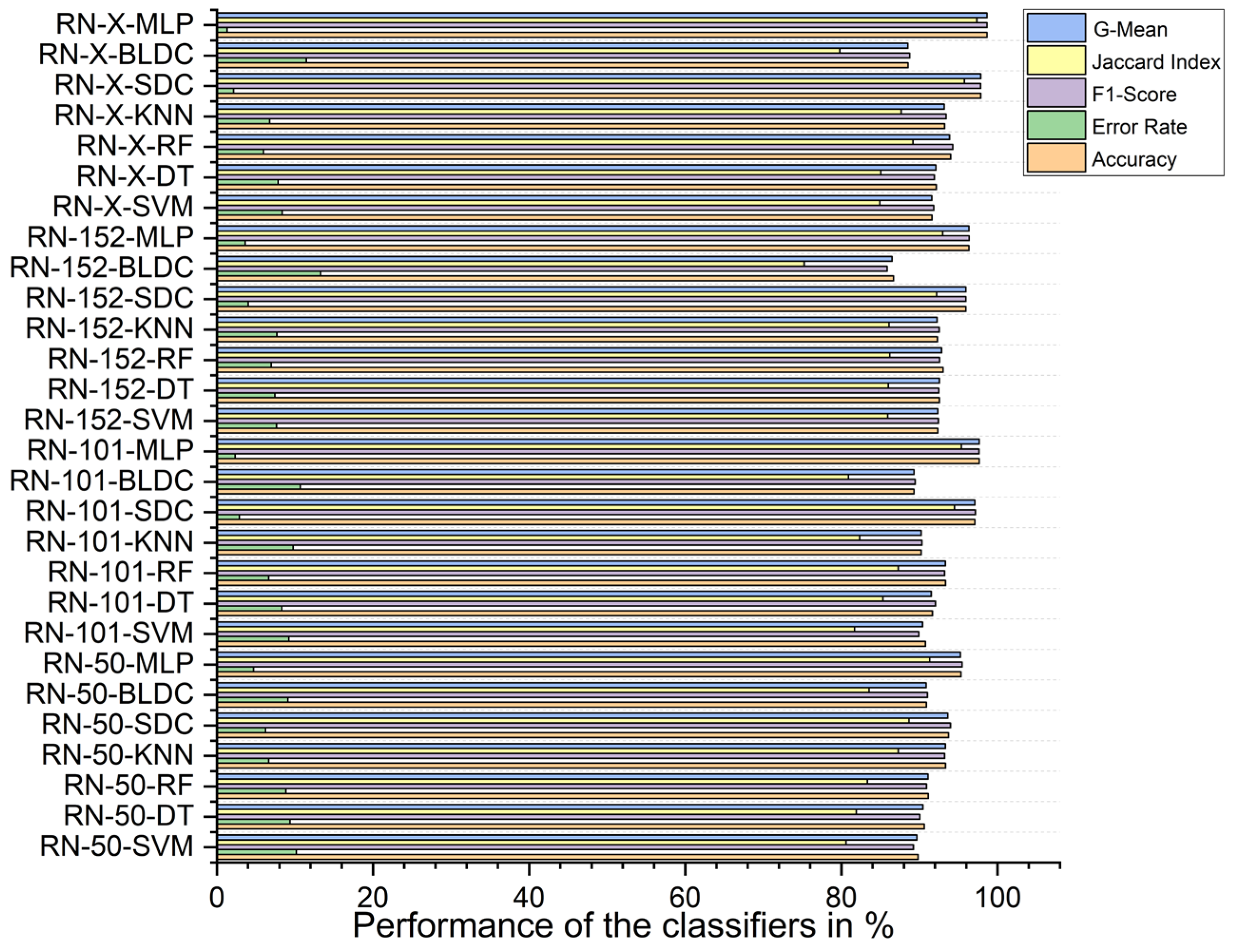
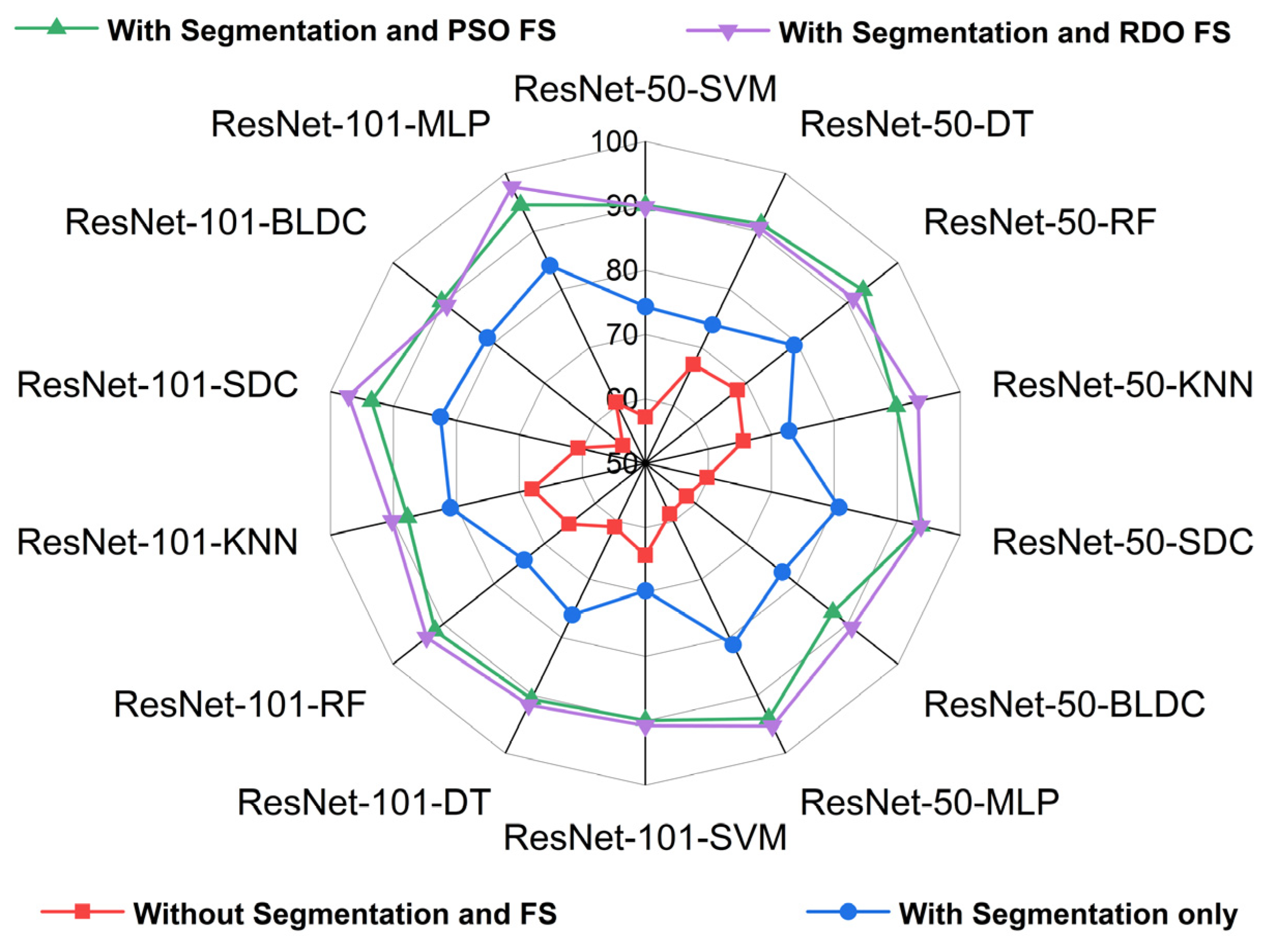
5.4. Performance Analysis of Classifiers for K = 10
5.5. Major Outcomes and Limitations
5.6. Computational Complexity
6. Conclusions
Author Contributions
Funding
Institutional Review Board Statement
Informed Consent Statement
Data Availability Statement
Conflicts of Interest
References
- Who Report on Cancer: Setting Priorities, Investing Wisely and Providing Care for All 2020. Available online: http://apps.who.int/bookorders (accessed on 24 February 2024).
- Siegel, R.L.; Giaquinto, A.N.; Jemal, A. Cancer statistics, 2024. CA Cancer J. Clin. 2024, 74, 12–49. [Google Scholar] [CrossRef] [PubMed]
- Sung, H.; Ferlay, J.; Siegel, R.L.; Laversanne, M.; Soerjomataram, I.; Jemal, A.; Bray, F. Global Cancer Statistics 2020: GLOBOCAN Estimates of Incidence and Mortality Worldwide for 36 Cancers in 185 Countries. CA Cancer J. Clin. 2021, 71, 209–249. [Google Scholar] [CrossRef] [PubMed]
- Araghi, M.; Soerjomataram, I.; Jenkins, M.; Brierley, J.; Morris, E.; Bray, F.; Arnold, M. Global trends in colorectal cancer mortality: Projections to the year 2035. Int. J. Cancer 2019, 144, 2992–3000. [Google Scholar] [CrossRef] [PubMed]
- WHO Classification of Tumours Editorial Board (Ed.) WHO Classification of Tumours. In Thoracic Tumours, 5th ed.; International Agency for Research on Cancer: Lyon, France, 2021; ISBN 978-92-832-4506-3. [Google Scholar]
- Andreadis, D.A.; Pavlou, A.M.; Panta, P. Biopsy and oral squamous cell carcinoma histopathology. In Oral Cancer Detection: Novel Strategies and Clinical Impact; Springer International Publishing: Berlin/Heidelberg, Germany, 2019; pp. 133–151. [Google Scholar] [CrossRef]
- Ozdemir, O.; Russell, R.L.; Berlin, A.A. A 3D Probabilistic Deep Learning System for Detection and Diagnosis of Lung Cancer Using Low-Dose CT Scans. IEEE Trans Med. Imaging 2020, 39, 1419–1429. [Google Scholar] [CrossRef]
- Teramoto, A.; Tsukamoto, T.; Kiriyama, Y.; Fujita, H. Automated Classification of Lung Cancer Types from Cytological Images Using Deep Convolutional Neural Networks. Biomed Res. Int. 2017, 2017, 4067832. [Google Scholar] [CrossRef]
- Anthimopoulos, M.; Christodoulidis, S.; Ebner, L.; Christe, A.; Mougiakakou, S. Lung Pattern Classification for Interstitial Lung Diseases Using a Deep Convolutional Neural Network. IEEE Trans Med. Imaging 2016, 35, 1207–1216. [Google Scholar] [CrossRef]
- Iizuka, O.; Kanavati, F.; Kato, K.; Rambeau, M.; Arihiro, K.; Tsuneki, M. Deep Learning Models for Histopathological Classification of Gastric and Colonic Epithelial Tumours. Sci. Rep. 2020, 10, 1504. [Google Scholar] [CrossRef]
- Wang, S.; Wang, T.; Yang, L.; Yang, D.M.; Fujimoto, J.; Yi, F.; Luo, X.; Yang, Y.; Yao, B.; Lin, S.; et al. ConvPath: A software tool for lung adenocarcinoma digital pathological image analysis aided by a convolutional neural network. EBioMedicine 2019, 50, 103–110. [Google Scholar] [CrossRef]
- Gessert, N.; Nielsen, M.; Shaikh, M.; Werner, R.; Schlaefer, A. Skin lesion classification using ensembles of multi-resolution EfficientNets with meta data. MethodsX 2020, 7, 100864. [Google Scholar] [CrossRef]
- Liu, Y.; Liu, X.; Qi, Y. Adaptive Threshold Learning in Frequency Domain for Classification of Breast Cancer Histopathological Images. Int. J. Intell. Syst. 2024, 1–13. [Google Scholar] [CrossRef]
- Zhou, Y.; Zhang, C.; Gao, S. Breast Cancer Classification from Histopathological Images Using Resolution Adaptive Network. IEEE Access 2022, 10, 35977–35991. [Google Scholar] [CrossRef]
- Wang, P.; Wang, J.; Li, Y.; Li, P.; Li, L.; Jiang, M. Automatic classification of breast cancer histopathological images based on deep feature fusion and enhanced routing. Biomed. Signal Process Control 2021, 65, 102341. [Google Scholar] [CrossRef]
- Aresta, G.; Araújo, T.; Kwok, S.; Chennamsetty, S.S.; Safwan, M.; Alex, V.; Aguiar, P. BACH: Grand challenge on breast cancer histology images. Med. Image Anal. 2019, 56, 122–139. [Google Scholar] [CrossRef]
- Spanhol, F.A.; Oliveira, L.S.; Petitjean, C.; Heutte, L. Breast cancer histopathological image classification using Convolutional Neural Networks. In Proceedings of the 2016 International Joint Conference on Neural Networks (IJCNN), Vancouver, BC, Canada, 24–29 July 2016; pp. 2560–2567. [Google Scholar] [CrossRef]
- Filipczuk, P.; Fevens, T.; Krzyzak, A.; Monczak, R. Computer-aided breast cancer diagnosis based on the analysis of cytological images of fine needle biopsies. IEEE Trans Med. Imaging 2013, 32, 2169–2178. [Google Scholar] [CrossRef]
- Mobark, N.; Hamad, S.; Rida, S.Z. CoroNet: Deep Neural Network-Based End-to-End Training for Breast Cancer Diagnosis. Appl. Sci. 2022, 12, 7080. [Google Scholar] [CrossRef]
- Araújo, T.; Aresta, G.; Castro, E.; Rouco, J.; Aguiar, P.; Eloy, C.; Campilho, A. Classification of breast cancer histology images using convolutional neural networks. PLoS ONE 2017, 12, 6. [Google Scholar] [CrossRef]
- Rafiq, A.; Chursin, A.; Awad Alrefaei, W.; Rashed Alsenani, T.; Aldehim, G.; Abdel Samee, N.; Menzli, L.J. Detection and Classification of Histopathological Breast Images Using a Fusion of CNN Frameworks. Diagnostics 2023, 13, 1700. [Google Scholar] [CrossRef]
- Hameed, Z.; Zahia, S.; Garcia-Zapirain, B.; Aguirre, J.J.; Vanegas, A.M. Breast cancer histopathology image classification using an ensemble of deep learning models. Sensors 2020, 20, 4373. [Google Scholar] [CrossRef]
- Wang, P.; Hu, X.; Li, Y.; Liu, Q.; Zhu, X. Automatic cell nuclei segmentation and classification of breast cancer histopathology images. Signal Process. 2016, 122, 1–13. [Google Scholar] [CrossRef]
- Borkowski, A.A.; Bui, M.M.; Thomas, L.B.; Wilson, C.P.; Deland, L.A.; Mastorides, S.M. Lung and Colon Cancer Histopathological Image Dataset (LC25000). Available online: https://github.com/beamandrew/medical-data (accessed on 24 February 2024).
- Boumaraf, S.; Liu, X.; Zheng, Z.; Ma, X.; Ferkous, C. A new transfer learning-based approach to magnification dependent and independent classification of breast cancer in histopathological images. Biomed. Signal Process Control 2021, 63, 102192. [Google Scholar] [CrossRef]
- Achanta, R.; Shaji, A.; Smith, K.; Lucchi, A.; Fua, P.; Süsstrunk, S. SLIC superpixels compared to state-of-the-art superpixel methods. IEEE Trans Pattern Anal. Mach. Intell. 2012, 34, 2274–2281. [Google Scholar] [CrossRef]
- He, K.; Zhang, X.; Ren, S.; Sun, J. Deep Residual Learning for Image Recognition. In Proceedings of the IEEE Conference on Computer Vision and Pattern Recognition, Las Vegas, NV, USA, 27–30 June 2016; pp. 770–778. [Google Scholar] [CrossRef]
- Theckedath, D.; Sedamkar, R.R. Detecting Affect States Using VGG16, ResNet50 and SE-ResNet50 Networks. SN Comput. Sci. 2020, 1, 79. [Google Scholar] [CrossRef]
- Alinsaif, S.; Lang, J. Texture features in the Shearlet domain for histopathological image classification. BMC Med. Inf. Decis. Mak. 2020, 20, 312. [Google Scholar] [CrossRef] [PubMed]
- Goel, L.; Patel, P. Improving YOLOv6 using advanced PSO optimizer for weight selection in lung cancer detection and classification. Multimed. Tools Appl. 2024, 83, 78059–78092. [Google Scholar] [CrossRef]
- Fathollahi-Fard, A.M.; Hajiaghaei-Keshteli, M.; Tavakkoli-Moghaddam, R. Red deer algorithm (RDA): A new nature-inspired meta-heuristic. Soft Comput. 2020, 24, 14637–14665. [Google Scholar] [CrossRef]
- Pincus, S.M. Approximate entropy as a measure of system complexity. Proc. Natl. Acad. Sci. USA 1991, 88, 2297–2301. [Google Scholar] [CrossRef] [PubMed] [PubMed Central]
- Kosko, B. Fuzzy entropy and conditioning. Inf. Sci. 1986, 40, 165–174. [Google Scholar] [CrossRef]
- Rachel, V.M.; Chokkalingam, S. Efficiency of Decision Tree Algorithm for Lung Cancer CT-Scan Images Comparing with SVM Algorithm. In Proceedings of the 2022 3rd International Conference on Smart Electronics and Communication (ICOSEC), Trichy, India, 20–22 October 2022; pp. 1561–1565. [Google Scholar] [CrossRef]
- Lavanya, C.; Pooja, S.; Kashyap, A.H.; Rahaman, A.; Niranjan, S.; Niranjan, V. Novel Biomarker Prediction for Lung Cancer Using Random Forest Classifiers. Cancer Inform. 2023, 22, 11769351231167992. [Google Scholar] [CrossRef]
- Song, Y.; Huang, J.; Zhou, D.; Zha, H.; Giles, C.L. LNAI 4702—IKNN: Informative K-Nearest Neighbor Pattern Classification. In Lecture Notes in Computer Science; Springer: Berlin/Heidelberg, Germany, 2007; Volume 4702. [Google Scholar] [CrossRef]
- Zang, F.; Zhang, J.S. Softmax discriminant classifier. In Proceedings of the 3rd International Conference on Multimedia Information Networking and Security, MINES 2011, Shanghai, China, 4–6 November 2011; pp. 16–19. [Google Scholar] [CrossRef]
- Liu, M.; Li, L.; Wang, H.; Guo, X.; Liu, Y.; Li, Y.; Song, K.; Shao, Y.; Wu, F.; Zhang, J.; et al. A multilayer perceptron-based model applied to histopathology image classification of lung adenocarcinoma subtypes. Front. Oncol. 2023, 13, 1172234. [Google Scholar] [CrossRef]
- Cybenko, G. Approximation by superpositions of a sigmoidal function. Math. Control Signal Syst. 1989, 2, 303–314. [Google Scholar] [CrossRef]
- Kalaiyarasi, M.; Rajaguru, H.; Ravi, S. PFCM Approach for Enhancing Classification of Colon Cancer Tumors using DNA Microarray Data. In Proceedings of the 2023 Third International Conference on Smart Technologies, Communication and Robotics (STCR), Sathyamangalam, India, 9–10 December 2023; pp. 1–6. [Google Scholar] [CrossRef]
- Jain, D.K.; Lakshmi, K.M.; Varma, K.P.; Ramachandran, M.; Bharati, S. Lung Cancer Detection Based on Kernel PCA-Convolution Neural Network Feature Extraction and Classification by Fast Deep Belief Neural Network in Disease Management Using Multimedia Data Sources. Comput. Intell. Neurosci. 2022, 2022, 3149406. [Google Scholar] [CrossRef] [PubMed]
- Civit-Masot, J.; Bañuls-Beaterio, A.; Domínguez-Morales, M.; Rivas-Pérez, M.; Muñoz-Saavedra, L.; Corral, J.M.R. Non-small cell lung cancer diagnosis aid with histopathological images using Explainable Deep Learning techniques. Comput. Methods Programs Biomed. 2022, 226, 107108. [Google Scholar] [CrossRef]
- Naseer, I.; Masood, T.; Akram, S.; Jaffar, A.; Rashid, M.; Iqbal, M.A. Lung Cancer Detection Using Modified AlexNet Architecture and Support Vector Machine. Comput. Mater. Contin. 2023, 74, 2039–2054. [Google Scholar] [CrossRef]
- Wang, Z.; Bi, Y.; Pan, T.; Wang, X.; Bain, C.; Bassed, R.; Song, J. Targeting tumor heterogeneity: Multiplex-detection-based multiple instances learning for whole slide image classification. Bioinformatics 2023, 39, btad114. [Google Scholar] [CrossRef]
- Masud, M.; Sikder, N.; Al Nahid, A.; Bairagi, A.K.; Alzain, M.A. A machine learning approach to diagnosing lung and colon cancer using a deep learning-based classification framework. Sensors 2021, 21, 748. [Google Scholar] [CrossRef]
- Wahid, R.R.; Nisa, C.; Amaliyah, R.P.; Puspaningrum, E.Y. Lung and colon cancer detection with convolutional neural networks on histopathological images. In AIP Conference Proceedings; American Institute of Physics Inc.: College Park, MD, USA, 2023. [Google Scholar] [CrossRef]
- Gupta, S.; Gupta, M.K.; Shabaz, M.; Sharma, A. Deep Learning Techniques for Cancer Classification Using Microarray Gene Expression Data; Frontiers Media S.A.: Lausanne, Switzerland, 2022. [Google Scholar] [CrossRef]
- Liu, Y.; Wang, H.; Song, K.; Sun, M.; Shao, Y.; Xue, S.; Zhang, T. CroReLU: Cross-Crossing Space-Based Visual Activation Function for Lung Cancer Pathology Image Recognition. Cancers 2022, 14, 5181. [Google Scholar] [CrossRef]
- Wang, X.; Yu, G.; Yan, Z.; Wan, L.; Wang, W.; Cui, L. Lung Cancer Subtype Diagnosis by Fusing Image-Genomics Data and Hybrid Deep Networks. IEEE/ACM Trans Comput. Biol. Bioinform 2023, 20, 512–523. [Google Scholar] [CrossRef]
- Mastouri, R.; Khlifa, N.; Neji, H.; Hantous-Zannad, S. A bilinear convolutional neural network for lung nodules classification on CT images. Int. J. Comput. Assist. Radiol. Surg. 2021, 16, 91–101. [Google Scholar] [CrossRef]
- Phankokkruad, M. Ensemble Transfer Learning for Lung Cancer Detection. In Proceedings of the ACM International Conference Proceeding Series, Montreal, Canada, 18–22 October 2021; Association for Computing Machinery: New York, NY, USA, 2021; pp. 438–442. [Google Scholar] [CrossRef]
- Bukhari, S.U.K.; Syed, A.; Bokhari, S.K.A.; Hussain, S.S.; Armaghan, S.U.; Shah, S.S.H. The Histological Diagnosis of Colonic Adenocarcinoma by Applying Partial Self Supervised Learning. medRxiv 2020, arXiv:15.20175760. [Google Scholar] [CrossRef]
- Anjum, S.; Ahmed, I.; Asif, M.; Aljuaid, H.; Alturise, F.; Ghadi, Y.Y.; Elhabob, R. Lung Cancer Classification in Histopathology Images Using Multiresolution Efficient Nets. Comput. Intell. Neurosci. 2023, 2023, 7282944. [Google Scholar] [CrossRef]
- Shourie, P.; Anand, V.; Gupta, S. Colon and Lung Cancer Classification of Histopathological Images Using Efficientnetb7. In Proceedings of the 2023 3rd Asian Conference on Innovation in Technology (ASIANCON), Ravet, India, 25–27 August 2023; pp. 1–5. [Google Scholar] [CrossRef]
- Diosdado, J.; Gilabert, P.; Seguí, S.; Borrego, H. LungHist700: A dataset of histological images for deep learning in pulmonary pathology. Sci. Data 2024, 11, 1088. [Google Scholar] [CrossRef]


| ResNet Architectures | A | B | C | D |
|---|---|---|---|---|
| RN-50 | 3 | 4 | 6 | 3 |
| RN-101 | 3 | 4 | 23 | 3 |
| RN-152 | 3 | 8 | 36 | 3 |
| Statistical Parameters | ResNet-50 | ResNet-101 | ResNet-152 | DWAFF- ResNet-X | ||||
|---|---|---|---|---|---|---|---|---|
| N | ACA | N | ACA | N | ACA | N | ACA | |
| Mean | 0.3384 | 0.3429 | 0.3444 | 0.3347 | 0.3508 | 0.3419 | 0.4538 | 0.4537 |
| Variance | 0.7147 | 0.8100 | 0.7920 | 0.8463 | 0.7987 | 0.8655 | 0.3807 | 0.4445 |
| Skewness | 5.4461 | 5.9408 | 5.4387 | 6.0005 | 5.5525 | 6.2248 | 3.7679 | 4.4868 |
| Kurtosis | 43.6833 | 52.9968 | 42.8377 | 52.9611 | 46.3895 | 60.2777 | 21.1486 | 33.4781 |
| PCC | 0.4994 | 0.5272 | 0.4958 | 0.5167 | 0.4944 | 0.5185 | 0.9386 | 0.9443 |
| Dice Coefficient | 0.7512 | 0.7043 | 0.8028 | 0.7557 | 0.8598 | 0.8011 | 0.9038 | 0.8572 |
| CCA | 0.7018 | 0.7532 | 0.8293 | 0.8816 | ||||
| S. No. | Parameters | Value | S. No. | Parameters | Value |
|---|---|---|---|---|---|
| 1 | Number of Populations | 100 | 6 | Beta | 0.5 |
| 2 | Simulation Time | 13 (s) | 7 | Gamma | 0.6 |
| 3 | Number of Male RDs | 12 | 8 | Roar | 0.23 |
| 4 | Number of Hinds | 58 | 9 | Fight | 0.47 |
| 5 | Alpha | 0.9 | 10 | Mating | 0.78 |
| Statistical Measures | PSO | RDO | ||
|---|---|---|---|---|
| N | ACA | N | ACA | |
| Approximate Entropy | 1.2385 | 1.7816 | 2.0123 | 2.4893 |
| Shannon Entropy | 3.8523 | 4.9891 | 5.0821 | 5.8982 |
| Fuzzy Entropy | 0.4862 | 0.5231 | 0.7283 | 0.9182 |
| Hyperparameters | ResNet-50 | ResNet-101 | ResNet-152 | DWAFF (Proposed Method) |
|---|---|---|---|---|
| Optimizer | Adam | Adam | Adam | Adam |
| Momentum | 0.8 | 0.85 | 0.9 | 0.95 |
| Initial Learning Rate | 0.05 | 0.03 | 0.01 | 0.001 |
| Learning Rate Decay | 1/10 every 4 Epochs | 1/10 every 6 Epochs | 1/10 every 8 Epochs | 1/10 every 10 Epochs |
| Weight Decay | 0.0005 | 0.0003 | 0.0001 | 0.00005 |
| Batch Size | 128 | 128 | 128 | 128 |
| Pooling Type | Global Average Pooling | Global Average Pooling | Global Average Pooling | Feature Fusion (DWAFF) |
| Total Epochs | 16 | 16 | 16 | 16 |
| Learning Rate Schedule | 0.05 → 0.005 (Epoch 4) → 0.0005 (Epoch 8) → 0.00005 (Epoch 12) | 0.03 → 0.003 (Epoch 6) → 0.0003 (Epoch 12) | 0.01 → 0.001 (Epoch 8) → 0.0001 (Epoch 16) | 0.001 → 0.0005 (Epoch 10) → 0.0001 (Epoch 16) |
| Classifiers | Description |
|---|---|
| SVM | Kernel function—RBF; support vector coefficient, α = 1.8; Gaussian function bandwidth (σ) = 98; bias term (b) = 0.012; convergence criterion—MSE. |
| KNN | K-5; distance metric—Euclidian; weight—0.52; criterion—MSE. |
| RF | Number of trees—150; maximum depth—15; bootstrap sample size—16; class weight—0.35. |
| DT | Maximum depth—14; impurity criterion—MSE; class weight—0.25. |
| SDC | λ—0.458, along with the average target values for each class being 0.15 and 0.85. |
| MLP | Learning rate—0.45; training method—LM; criterion—MSE. |
| BLDC | Mean and Covariance matrix are calculated with a prior probability of 0.12; convergence criteria = MSE. |
| Performance Metrics | Equation | Significance |
|---|---|---|
| Accuracy (%) | The overall accuracy of the classifier’s predictions. | |
| Error rate (%) | The ratio of misclassified instances | |
| F1 score (%) | The harmonic mean of precision and recall, reflecting the classification accuracy for a specific class | |
| MCC | The Pearson correlation between the observed and predicted classifications | |
| Jaccard index (%) | The proportion of predicted true positives to the sum of predicted true positives and actual positives, regardless of their true or predicted status | |
| G-mean (%) | A metric combines sensitivity and specificity into a singular value balancing both objectives | |
| Kappa | Evaluates how well the observed and predicted classifications align, reflecting the consistency of the classification outcomes |
| S. No. | Authors | Dataset Used | Classification Models | Accuracy (%) | Challenges |
|---|---|---|---|---|---|
| 1 | Jain et al. (2022) [41] | 1500 images from LZ2500 dataset | Kernel PCA combined with faster deep belief networks | 97.10% | Data availability, computational complexity and generalizability across different medical centers |
| 2 | Civit-Masot et al. (2022) [42] | 15,000 images from LC25000 dataset | Custom architecture with three convolutional and two dense layers | 99.69% with 50 epochs | Overfitting risk due to high accuracy, lack of clinical validation, dataset bias |
| 3 | Iftikhar Naseer et al. (2023) [43] | LUNA 16 Database | LungNet-SVM | 97.64% | Limited dataset, potential model bias, difficulty in handling real-world noise in CT scans |
| 4 | Wang et al. (2023) [44] | 993 WSIs from TCGA dataset | A novel multiplex detection-based MIL model | 90.52% | Complexity in handling whole-slide images (WSIs), interpretability issues in MIL-based models |
| 5 | Mehedi Masud et al. (2021) [45] | LC25000 dataset | Custom CNN architecture consisting of three convolutional layers and one FC layer | 96.33% | Lack of robustness to dataset variability, potential overfitting, limited feature extraction |
| 6 | Radical Rakhman Wahid et al. (2023) [46] | LC25000 Database | Customized CNN model | 93.02% | Computational inefficiency, insufficient testing on real-world medical images |
| 7 | Gupta et al. (2022) [47] | TCGA dataset | Deep CNN | 92% | High data variability in TCGA, lack of interpretability in deep CNNs |
| 8 | Liu et al. (2022) [48] | 766 lung WSIs from First Hospital of Baiqiu’en and LC25000 dataset | SE-ResNet-50 with novel activation function CroRELU | 98.33% | Computationally intensive, risk of overfitting with small dataset, limited clinical validation |
| 9 | Wang et al. (2023) [49] | 988 samples with both CNV and histological data | LungDIG: combination of InceptionV3 with MLP | 87.10% | Low accuracy compared to other models, difficulty in integrating CNV data with histological features |
| 10 | Mastouri et al. (2021) [50] | LUNA16 Database (3186 CT images) | BCNN [VGG16, VGG19] | 91.99% | Pretrained VGG models may not generalize well, requires fine-tuning, dataset-specific performance |
| 11 | Phankokkruad (2021) [51] | LC25000 Database | Ensemble ResNet50V2 | 91% 90% | Ensemble models require higher computational resources, longer training time |
| 12 | Bukhari et al. (2020) [52] | CRAG Dataset | ResNet-50 | 93.91% | Requires large datasets to avoid overfitting, difficulty in domain adaptation |
| 13 | Sunila Anjum et al. (2023) [53] | LC25000 Database | EfficientNet (B0 to B7) | 97% | EfficientNet may struggle with small datasets, needs proper tuning for histopathological images |
| 14 | Poonam Shourie et al. (2023) [54] | LC25000 Database | EfficientNet B7 | 98.49% | High computational cost, requires a large dataset for better generalization |
| 15 | Joge Diosdado et al. (2024) [55] | LungHist700 | DNN and MIL | 81–92% | Dataset size limitation, MIL-approach complexity, difficulty in model explainability |
| 16 | Karthikeyan Shanmugam, Harikumar Rajaguru This research | LC25000 Database | Feature extraction—RDO in selective feature layer—ResNet-X framework with MLP classifier | 98.698% | — |
| Deep Feature Extraction—Architectures | Classifiers | Without Segmentation | With Segmentation | With Segmentation and PSO Feature Selection | With Segmentation and RDO Feature Selection |
|---|---|---|---|---|---|
| ResNet-50 | SVM | ||||
| DT | |||||
| RF | |||||
| KNN | |||||
| SDC | |||||
| BLDC | |||||
| MLP | |||||
| ResNet-101 | SVM | ||||
| DT | |||||
| RF | |||||
| KNN | |||||
| SDC | |||||
| BLDC | |||||
| MLP | |||||
| ResNet-152 | SVM | ||||
| DT | |||||
| RF | |||||
| KNN | |||||
| SDC | |||||
| BLDC | |||||
| MLP | |||||
| DWAFF— ResNet-X | SVM | ||||
| DT | |||||
| RF | |||||
| KNN | |||||
| SDC | |||||
| BLDC | |||||
| MLP |
Disclaimer/Publisher’s Note: The statements, opinions and data contained in all publications are solely those of the individual author(s) and contributor(s) and not of MDPI and/or the editor(s). MDPI and/or the editor(s) disclaim responsibility for any injury to people or property resulting from any ideas, methods, instructions or products referred to in the content. |
© 2025 by the authors. Licensee MDPI, Basel, Switzerland. This article is an open access article distributed under the terms and conditions of the Creative Commons Attribution (CC BY) license (https://creativecommons.org/licenses/by/4.0/).
Share and Cite
Shanmugam, K.; Rajaguru, H. Enhanced Superpixel-Guided ResNet Framework with Optimized Deep-Weighted Averaging-Based Feature Fusion for Lung Cancer Detection in Histopathological Images. Diagnostics 2025, 15, 805. https://doi.org/10.3390/diagnostics15070805
Shanmugam K, Rajaguru H. Enhanced Superpixel-Guided ResNet Framework with Optimized Deep-Weighted Averaging-Based Feature Fusion for Lung Cancer Detection in Histopathological Images. Diagnostics. 2025; 15(7):805. https://doi.org/10.3390/diagnostics15070805
Chicago/Turabian StyleShanmugam, Karthikeyan, and Harikumar Rajaguru. 2025. "Enhanced Superpixel-Guided ResNet Framework with Optimized Deep-Weighted Averaging-Based Feature Fusion for Lung Cancer Detection in Histopathological Images" Diagnostics 15, no. 7: 805. https://doi.org/10.3390/diagnostics15070805
APA StyleShanmugam, K., & Rajaguru, H. (2025). Enhanced Superpixel-Guided ResNet Framework with Optimized Deep-Weighted Averaging-Based Feature Fusion for Lung Cancer Detection in Histopathological Images. Diagnostics, 15(7), 805. https://doi.org/10.3390/diagnostics15070805