

A Machine-Learning-Based Analysis of Resting State Electroencephalogram Signals to Identify Latent Schizotypal and Bipolar Development in Healthy University Students
 , , , , , , and
Abstract
1. Introduction
2. State of the Art
3. Materials and Methods
3.1. Subjects
3.2. Assessments
3.3. Recording Procedure
3.4. Data Preprocessing
3.5. Data Analysis
3.5.1. Microstate Analysis
3.5.2. Frequency Domain Analysis
3.6. Machine Learning
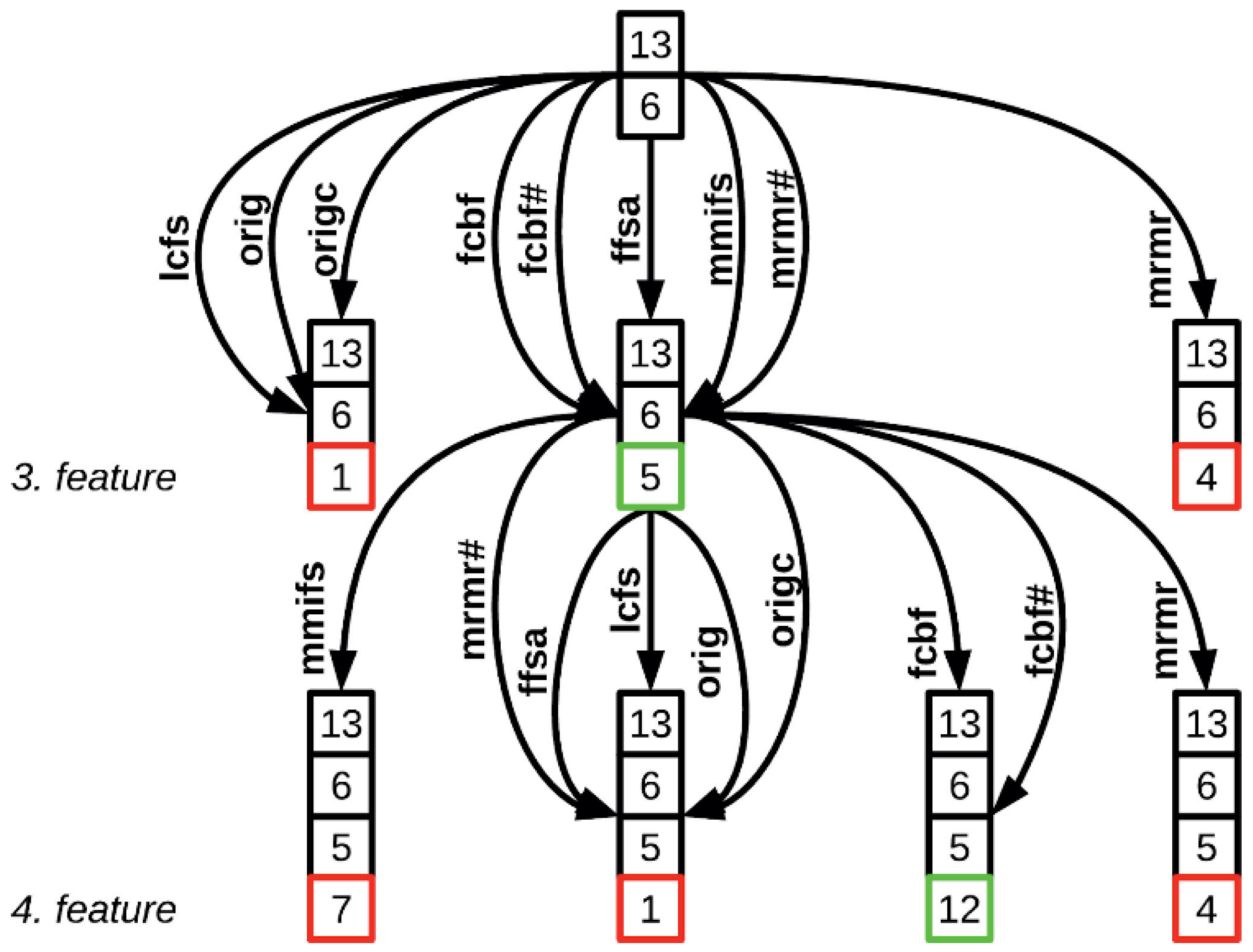
3.6.1. AHFS
3.6.2. Clique Forming Feature Selection
4. Results
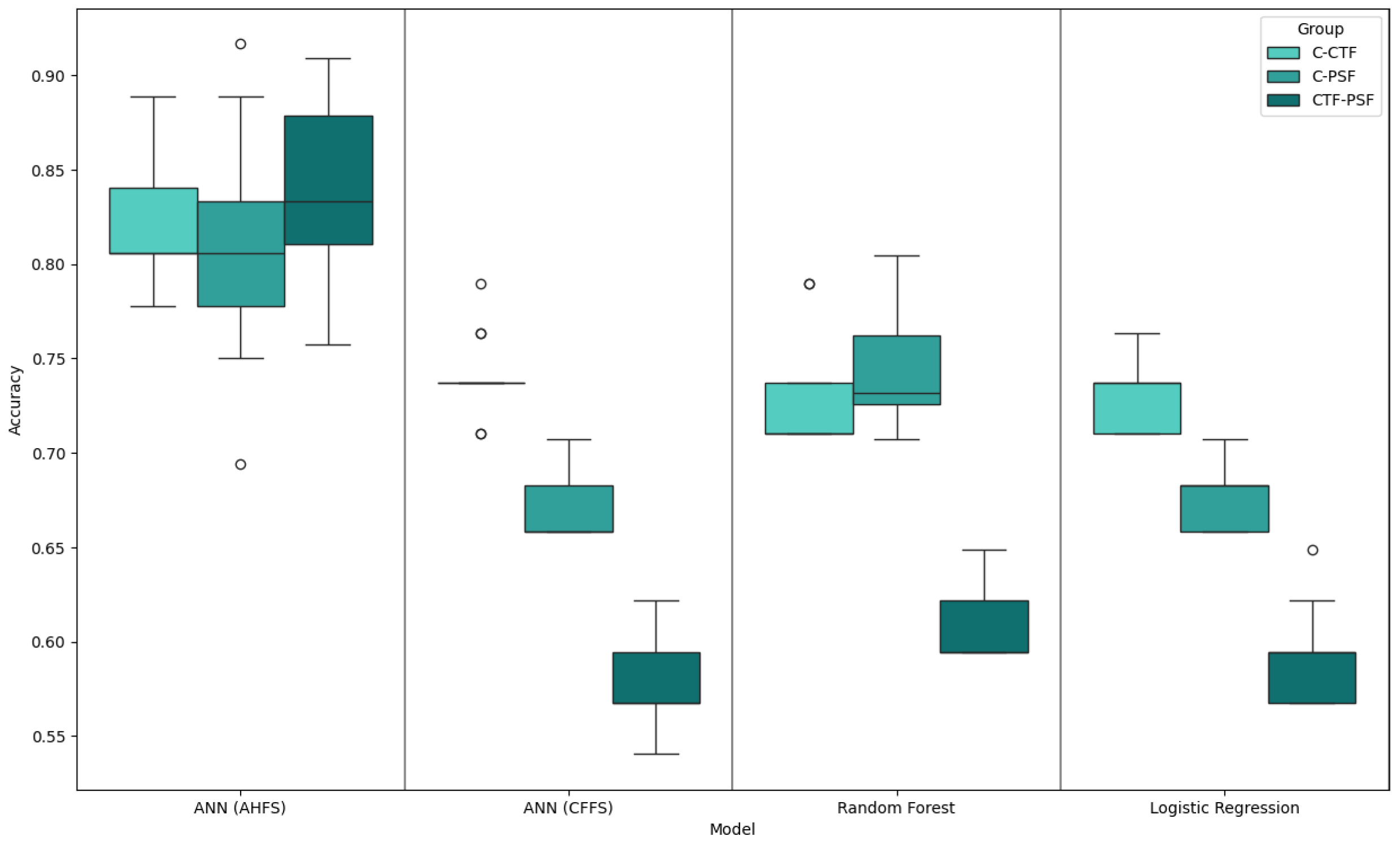
4.1. Generated Models
4.2. PSF Group Findings
4.3. CTF Group Findings
4.4. CTF-PSF Comparison Findings
5. Discussion
5.1. Frequency Bands
5.2. Complexity
5.3. Additional Features
5.4. Localization of the Features
5.5. Features of the PSF Group
5.6. Features of the CTF Group
5.7. PSF-CTF Comparison
5.8. Microstates
5.9. Comparison of Results
6. Conclusions
Limitations
Author Contributions
Funding
Institutional Review Board Statement
Informed Consent Statement
Data Availability Statement
Acknowledgments
Conflicts of Interest
Abbreviations
| AI | Artificial Intelligence |
| ANN | Artificial Neural Network |
| AHFS | Adaptive Hybrid Feature Selection |
| BA | Brodmann Area |
| BD | Bipolar Disorder |
| BIS/BAS | Behavioral Inhibition and Activation System |
| C | Control Group |
| CFFS | Clique Forming Feature Selection |
| CNN | Convolutional Neural Network |
| CTF | CycloThymia Factor group |
| DFA | Detrended Fluctuation Analysis |
| DIT | Direct Information Theory |
| DT | Decision Trees |
| EASE | Examination of Anomalous Self-experiences |
| EEG | Electroencephalogram |
| ERP | Event Related Potential |
| fMRI | functional Magnetic Resonance Imaging |
| GFP | Global Field Power |
| HFD | Higuchi Fractal Dimension |
| ICA | Independent Component Analysis |
| LAPS | Leuven Affect and Pleasure Scale |
| LR | Logistic Regression |
| LZC | Lempel-Ziv Complexity |
| MDQ | Mood Disorder Questionnaire |
| MEQ-SA | Morningness Eveningness Questionnaire |
| MS | Microstates |
| NN | Neural Network |
| O-LIFE | Oxford-Liverpool Inventory of Feelings and Experiences |
| PDI | Peters Delusions Inventory |
| PSD | Power Spectral Density |
| PSF | Positive Schizotypy Factor Group |
| RF | Random Forest |
| rsEEG | resting-state Electroencephalogram |
| sampEn | Sample Entropy |
| SCID | Structured Clinical Interview for DSM |
| SVM | Support Vector Machines |
| SZ | Schizophrenia |
| TCI-R | Temperament and Character Inventory |
| TEMPS-A | Temperament Evaluation of Memphis, Pisa, Paris, and San Diego Autoquestionnaire |
Appendix A. Additional Figures and Tables


| Feature Type | Number of Features per Sample | Feature Names |
|---|---|---|
| Transition Matrix | 16 | AA, AB, AC, AD, BA, BB, BC, BD, CA, CB, CC, CD, DA, DB, DC, DD |
| Symmetry Test | 1 | symmetry_p |
| Markov Tests (Zero-, First-, and Second-Order) | 3 | markov0_p, markov1_p, markov2_p |
| DIT Calculations | 6 | prob_a, prob_b, prob_c, prob_d, dit_extropy, dit_shannon_entropy |
| Conditional Homogeneity Test | 9 | homogenity_p_{l} |
| Hjorth Parameters | 384 (3 × 32 × 4) | hjorthActivity_{channel}_{stat}, hjorthMobility_{channel}_{stat}, hjorthComplexity_{channel}_{stat} |
| Power Spectral Density (PSD) | 4224 (32 × 33 × 4) | PSD_{channel}_{frequency}_{stat} |
| Lempel-Ziv Complexity (LZC) | 128 (32 × 4) | LZC_{channel}_{stat} |
| Detrended Fluctuation Analysis (DFA) | 128 (32 × 4) | DFA_{channel}_{stat} |
| Engagement Level | 4 | engagementLevel_{stat} |
| Higuchi Fractal Dimension (HFD) | 128 (32 × 4) | HFD_{channel}_{stat} |
| Sample Entropy | 128 (32 × 4) | sampEn_{channel}_{stat} |


| Microstate Features | Count of Feature Appearance | Average Point of the Feature |
|---|---|---|
| BC | 20 | 365 |
| CB | 20 | 360 |
| markov1_p | 20 | 324 |
| AD | 20 | 296 |
| homogenity_p_70 | 19 | 295 |
| prob_c | 20 | 282 |
| prob_e | 20 | 269 |
| CE | 20 | 267 |
| DA | 20 | 266 |
| Shannon_hk_3 | 20 | 249 |
| AA | 20 | 222 |
| prob_a | 20 | 193 |
| EC | 18 | 138 |
| symmetry_p | 19 | 114 |
| CD | 18 | 111 |
| AC | 18 | 108 |
| homogenity_p_65 | 14 | 98 |
| BD | 14 | 51 |
| homogenity_p_40 | 12 | 51 |
| EE | 12 | 49 |
| homogenity_p_45 | 7 | 25 |
| DC | 9 | 23 |
| Shannon_hk_2 | 8 | 18 |
| homogenity_p_50 | 5 | 12 |
| Shannon_hk_4 | 3 | 7 |
| homogenity_p_55 | 2 | 5 |
| DB | 1 | 1 |
| homogenity_p_60 | 1 | 1 |
Appendix B. Methodology Details
Appendix B.1. Utilized Learning Algorithms
- Logistic Regression (LR), as described by Gasso et al. (2012) [78], is a popular algorithm for binary classification tasks. In our study, we adopted LR for both feature selection and classification purposes. This algorithm was set up with an “l2” penalty metric alongside the “bilinear” solver. By fitting a linear regression model to our training dataset and then applying a logistic function, LR is able to generate probability values that aid in the classification of instances. Logistic regression offers a dependable approach for interpretable binary classification. Through the careful selection of penalty metrics and solvers, LR was efficiently utilized for feature selection and classification within our study. However, it should be mentioned that LR generally performs well with fewer features, so in the analysis it tended to select small feature sets as good ones.
- Random Forest (RF), described by Liaw et al. (2002) [79], embodies an ensemble learning technique where classification is achieved through majority voting from a collection of unpruned classification trees. These trees are developed from randomly selected subsets of the dataset, and at each decision node a randomly selected predictor determines the split, diverging from the conventional method of choosing the best split. Our implementation of RF involved the creation of 50 trees, employing the “auto” feature to cap the number of features evaluated at each split. We set the minimum number of samples required to split a node to 2, without imposing limits on the tree’s maximum depth or the maximum number of leaf nodes.
- Artificial Neural Network (ANN) sets the stage for a comparative analysis between CFFS and AHFS. Given that AHFS operates within a MATLAB framework and offers less flexibility, we endeavored to merge the neural network from AHFS into the CFFS framework. This integration met with partial success due to the inherent differences in the programming languages. The ANN is pivotal for our method comparison. The data normalization process began with the application of a min–max scaler, adjusting the dataset to a range between 0.1 and 0.9. The ANN’s structure included an input layer, succeeded by a single hidden layer with 8 neurons, in a first evaluation round; later, we found some overfitted models, so the neuron numbers were decreased to 3. During training, the bach size was 8 and early stopping was applied. This featured the sigmoid activation function and concluded with an output layer of two neurons using the softmax activation function to represent the binary classes. While the original AHFS method applied a specific optimizer, our Python adaptation used the Adam optimizer, due to the original optimizer’s incompatibility with the Python ecosystem.
Appendix B.2. Feature Selection Details
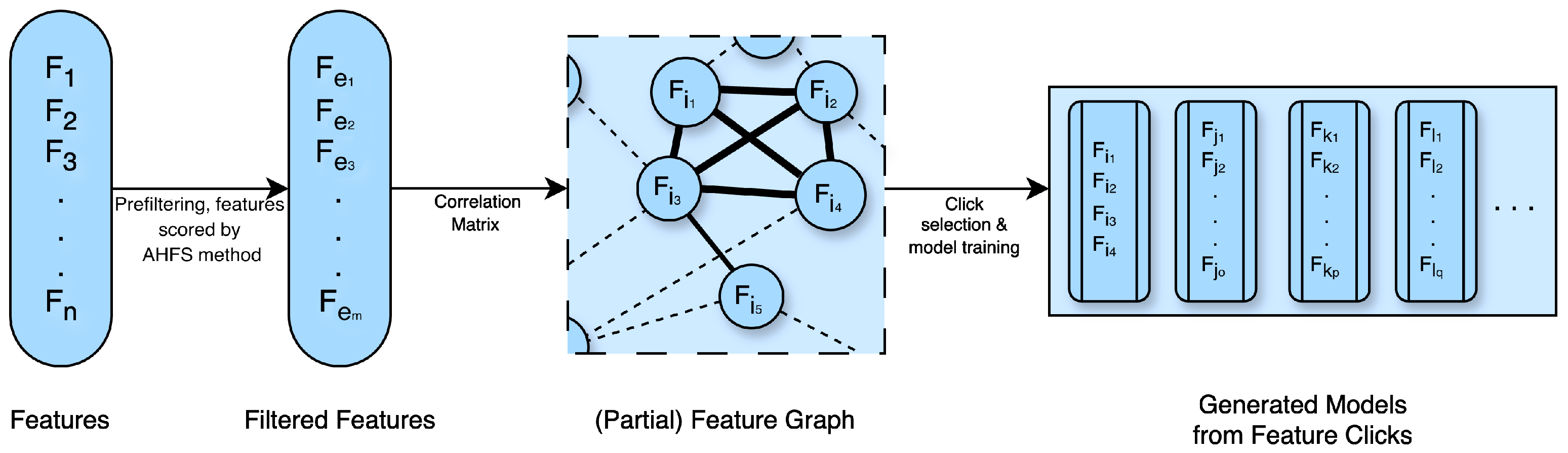
- Prefiltering: Due to the enormous amount of EEGlib features, The criteria to include a feature is to have at least one appear in the AHFS feature selection. Each run of the AHFS selected 20 features, and we applied 20 runs, therefore 400; in both cases, 35 unique features are selected in the process. All the microstate features were included in the feature selection.
- Weighed graph composition with Pearson correlation: From the remaining selected features, pairwise comparisons were made to compute Pearson correlations. This resulted in a complete weighted graph, with the removal of loop and double edges.
- Threshold-based edge deletion: Edges with weights in absolute values above a certain threshold were deleted from the graph. This threshold was 0.4 in the PSF group and 0.33 in the CTF group.
- Clique identification: The remaining graph was analyzed to identify cliques, which are complete sub-graphs where every node is connected to every other node. A large number of cliques, approximately 5000 in both cases, were found. From these, a random selection was made of up to 600 feature sets, choosing between 3 to 9 cliques of varying sizes.
- These cliques, identified through the feature selection process, served as the potential optimal combinations of features for training the three learning algorithms. During the learning process, Shapley values were computed, utilizing a 3-fold cross-validation approach. The resulting models were ranked according to their accuracy scores and the top 20 were selected for the next step.
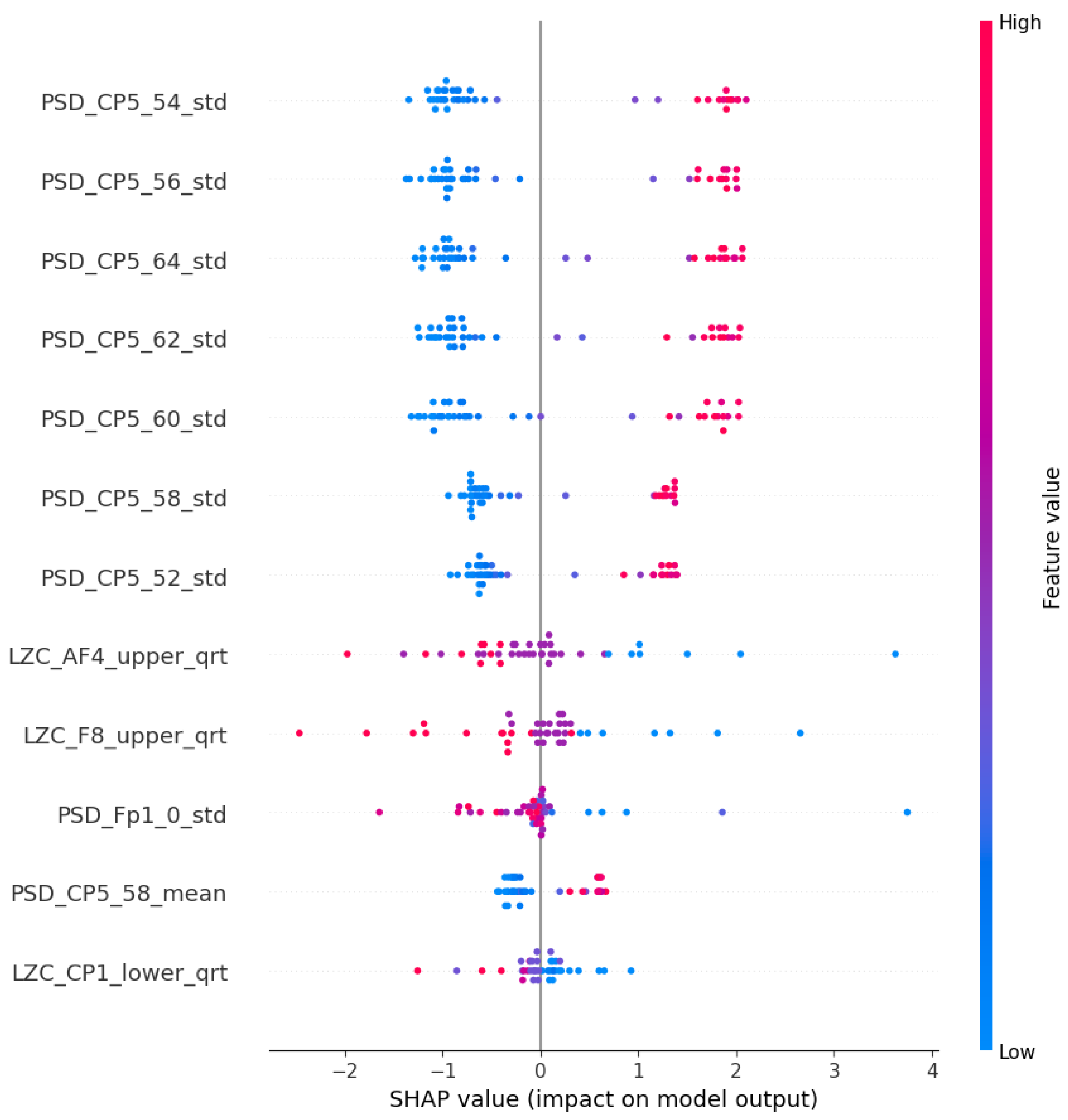
- For each model, a Shapley table was generated, consisting of columns representing the features included in the model, rows representing the individual samples, and values corresponding to the Shapley values. By aggregating the corresponding columns from each selected model, a comprehensive understanding of the model’s performance within the group was obtained. This aggregation process was conducted for models trained with each ML algorithm separately, ensuring the elimination of individual outliers and providing a robust depiction of the models’ functionality.
- Calculation demand: Step 1 is based upon the other algorithm. Steps 2 and 3 have minuscule computing and only need to be done once for each task. Step 4, searching for cliques in the 35-node graph, takes 20–40 s (also needs to be done once). The training of the 600 model with each three algorithms takes 400–450 min (depending on the size of the feature sets)—the different algorithms take different amounts of time to train. Shapely calculation and aggregation takes 20–30 min.
Appendix B.3. Feature Type Details
- Hjorth Parameters (Activity, Mobility, and Complexity) are computed in order to offer valuable insights into the variance, frequency attributes, and complexity of an EEG signal. Activity at Hjorth quantifies the variance, which indicates the overall strength of the signal. Hjorth mobility provides information regarding the frequency dynamics of a signal by measuring its mean frequency. Changes in frequency are utilized to quantify Hjorth complexity, which indicates the irregularity and complexity of the signal. After calculating these parameters for each of the 32 EEG channels, three features are produced per channel per chunk.
- Power Spectral Density (PSD) estimates the frequency-dependent power distribution of the EEG signal. PSD is computed within the interval of 0 to 64 Hz using a 2 Hz step size in our analysis, yielding 33 frequency bins.
- Sample Entropy (sampEn) of the EEG signal quantifies its irregularity and complexity. It measures the probability that analogous signal patterns will persist at a subsequent juncture. This attribute is computed for every single one of the 32 EEG channels.
- Lempel-Ziv Complexity (LZC) is a metric that quantifies the complexity of an EEG signal by assessing the quantity of unique patterns present in the signal. It is computed for every one of the 32 EEG channels.
- Detrended Fluctuation Analysis (DFA) is utilized to detect long-range correlations in the EEG signal. It is determined for every single one of the 32 EEG channels.
- Level of Engagement is an index that measures the degree of attention or engagement in accordance with the EEG signal. In contrast to the remaining features, engagement level generates a singular engagement score per interval by aggregating multiple features from all channels.
- Higuchi Fractal Dimension (HFD) is a method utilized to approximate the fractal dimension of an EEG signal, which serves as an indicator of the signal’s complexity. This attribute is computed for every single one of the 32 EEG channels.
References
- McGrath, J.; Saha, S.; Welham, J.; El Saadi, O.; MacCauley, C.; Chant, D. A systematic review of the incidence of schizophrenia: The distribution of rates and the influence of sex, urbanicity, migrant status and methodology. BMC Med. 2004, 2, 13. [Google Scholar] [CrossRef]
- Merikangas, K.R.; Akiskal, H.S.; Angst, J.; Greenberg, P.E.; Hirschfeld, R.M.; Petukhova, M.; Kessler, R.C. Lifetime and 12-month prevalence of bipolar spectrum disorder in the National Comorbidity Survey replication. Arch. Gen. Psychiatry 2007, 65, 543–552. [Google Scholar] [CrossRef] [PubMed]
- He, H.; Liu, Q.; Li, N.; Guo, L.; Gao, F.; Bai, L.; Gao, F.; Lyu, J. Trends in the incidence and DALYs of schizophrenia at the global, regional and national levels: Results from the Global Burden of Disease Study 2017. Epidemiol. Psychiatr. Sci. 2020, 29, e91. [Google Scholar] [CrossRef] [PubMed]
- He, H.; Hu, C.; Ren, Z.; Bai, L.; Gao, F.; Lyu, J. Trends in the incidence and DALYs of bipolar disorder at global, regional, and national levels: Results from the global burden of Disease Study 2017. J. Psychiatr. Res. 2020, 125, 96–105. [Google Scholar] [CrossRef] [PubMed]
- Barnhill, L.J. The diagnosis and treatment of individuals with mental illness and developmental disabilities: An overview. Psychiatr. Q. 2008, 79, 157–170. [Google Scholar] [CrossRef]
- Colombo, F.; Calesella, F.; Mazza, m.G.; Melloni, E.m.T.; Morelli, m.J.; Scotti, G.m.; Benedetti, F.; Bollettini, I.; Vai, B. Machine learning approaches for prediction of bipolar disorder based on biological, clinical and neuropsychological markers: A systematic review and meta-analysis. Neurosci. Biobehav. Rev. 2022, 135, 104552. [Google Scholar] [CrossRef] [PubMed]
- Rahul, J.; Sharma, D.; Sharma, L.D.; Nanda, U.; Sarkar, A.K. A systematic review of EEG based automated schizophrenia classification through machine learning and deep learning. Front. Hum. Neurosci. 2024, 18, 1347082. [Google Scholar] [CrossRef] [PubMed]
- Davis, J.; Maes, M.; Andreazza, A.; McGrath, J.; Tye, S.; Berk, M. Towards a classification of biomarkers of neuropsychiatric disease: From encompass to compass. Mol. Psychiatry 2015, 20, 152–153. [Google Scholar] [CrossRef]
- Trotta, A.; Murray, R.M.; MacCabe, J.H. Do premorbid and post-onset cognitive functioning differ between schizophrenia and bipolar disorder? A systematic review and meta-analysis. Psychol. Med. 2015, 45, 381–394. [Google Scholar] [CrossRef]
- Cannon, T.D.; Yu, C.; Addington, J.; Bearden, C.E.; Cadenhead, K.S.; Cornblatt, B.A.; Heinssen, R.; Jeffries, C.D.; Mathalon, D.H.; McGlashan, T.H.; et al. An individualized risk calculator for research in prodromal psychosis. Am. J. Psychiatry 2016, 173, 980–988. [Google Scholar] [CrossRef] [PubMed]
- Newson, J.J.; Thiagarajan, T.C. EEG frequency bands in psychiatric disorders: A review of resting state studies. Front. Hum. Neurosci. 2019, 12, 521. [Google Scholar] [CrossRef] [PubMed]
- Sargent, K.; Chavez-Baldini, U.; Master, S.L.; Verweij, K.J.; Lok, A.; Sutterland, A.L.; Vulink, N.C.; Denys, D.; Smit, D.J.; Nieman, D.H. Resting-state brain oscillations predict cognitive function in psychiatric disorders: A transdiagnostic machine learning approach. NeuroImage Clin. 2021, 30, 102617. [Google Scholar] [CrossRef]
- Rocca, D.L.; Campisi, P.; Vegso, B.; Cserti, P.; Kozmann, G.; Babiloni, F.; Fallani, F.D.V. Human Brain Distinctiveness Based on EEG Spectral Coherence Connectivity. IEEE Trans. Biomed. Eng. 2014, 61, 2406–2412. [Google Scholar] [CrossRef] [PubMed]
- Solomon, M. EEG Variabilities in Diagnosis of Schizophrenia, Bipolar Disorder, and PTSD: A Literature Review. J. Neurophysiol. Monit. 2023, 1, 1–11. [Google Scholar] [CrossRef]
- Babiloni, C.; Barry, R.J.; Başar, E.; Blinowska, K.J.; Cichocki, A.; Drinkenburg, W.H.; Klimesch, W.; Knight, R.T.; da Silva, F.L.; Nunez, P.; et al. International Federation of Clinical Neurophysiology (IFCN)–EEG research workgroup: Recommendations on frequency and topographic analysis of resting state EEG rhythms. Part 1: Applications in clinical research studies. Clin. Neurophysiol. 2020, 131, 285–307. [Google Scholar] [CrossRef]
- Perrottelli, A.; Giordano, G.m.; Brando, F.; Giuliani, L.; Mucci, A. EEG-Based Measures in At-Risk Mental State and Early Stages of Schizophrenia: A Systematic Review. Front. Psychiatry 2021, 12, 653642. [Google Scholar] [CrossRef]
- Koenig, T.; Prichep, L.; Lehmann, D.; Sosa, P.V.; Braeker, E.; Kleinlogel, H.; Isenhart, R.; John, E.R. Millisecond by millisecond, year by year: Normative EEG microstates and developmental stages. Neuroimage 2002, 16, 41–48. [Google Scholar] [CrossRef]
- Michel, C.M.; Koenig, T. EEG microstates as a tool for studying the temporal dynamics of whole-brain neuronal networks: A review. Neuroimage 2018, 180, 577–593. [Google Scholar] [CrossRef] [PubMed]
- Baradits, M.; Bitter, I.; Czobor, P. Multivariate patterns of EEG microstate parameters and their role in the discrimination of patients with schizophrenia from healthy controls. Psychiatry Res. 2020, 288, 112938. [Google Scholar] [CrossRef] [PubMed]
- Wang, F.; Hujjaree, K.; Wang, X. Electroencephalographic Microstates in Schizophrenia and Bipolar Disorder. Front. Psychiatry 2021, 12, 638722. [Google Scholar] [CrossRef] [PubMed]
- Nguyen, T.D.; Vo, V.T.; Ha, T.T.H. Bipolar disorder traits: An electroencephalogram systematic review. Minist. Sci. Technol. Vietnam 2022, 64, 84–90. [Google Scholar] [CrossRef]
- Payá, B.; Rodríguez-Sánchez, J.M.; Otero, S.; Muñoz, P.; Castro-Fornieles, J.; Parellada, M.; Gonzalez-Pinto, A.; Soutullo, C.; Baeza, I.; Rapado-Castro, M.; et al. Premorbid impairments in early-onset psychosis: Differences between patients with schizophrenia and bipolar disorder. Schizophr. Res. 2013, 146, 103–110. [Google Scholar] [CrossRef] [PubMed]
- Viharos, Z.; Kis, K.; Fodor, Á.; Büki, M. Adaptive, Hybrid Feature Selection (AHFS). Pattern Recognit. 2021, 116, 107932. [Google Scholar] [CrossRef]
- Nagy, A.; Dombi, J.; Fülep, m.P.; Rudics, E.; Hompoth, E.A.; Szabó, Z.; Dér, A.; Búzás, A.; Viharos, Z.J.; Hoang, A.T.; et al. The Actigraphy-Based Identification of Premorbid Latent Liability of Schizophrenia and Bipolar Disorder. Sensors 2023, 23, 958. [Google Scholar] [CrossRef]
- Jain, A.; Raja, R.; Srivastava, S.; Sharma, P.C.; Gangrade, J.; Manoy, R. Analysis of EEG signals and data acquisition methods: A review. Comput. Methods Biomech. Biomed. Eng. Imaging Vis. 2024, 12, 2304574. [Google Scholar] [CrossRef]
- Aslan, Z.; Akin, M. Automatic Detection of Schizophrenia by Applying Deep Learning over Spectrogram Images of EEG Signals. Trait. Du Signal 2020, 37, 235–244. [Google Scholar] [CrossRef]
- Barros, C.; Silva, C.A.; Pinheiro, A.P. Advanced EEG-based learning approaches to predict schizophrenia: Promises and pitfalls. Artif. Intell. Med. 2021, 114, 102039. [Google Scholar] [CrossRef]
- Yasin, S.; Hussain, S.A.; Aslan, S.; Raza, I.; Muzammel, M.; Othmani, A. EEG based Major Depressive disorder and Bipolar disorder detection using Neural Networks: A review. Comput. Methods Programs Biomed. 2021, 202, 106007. [Google Scholar] [CrossRef] [PubMed]
- Ravan, M.; Noroozi, A.; Sanchez, M.m.; Borden, L.; Alam, N.; Flor-Henry, P.; Hasey, G. Discriminating between bipolar and major depressive disorder using a machine learning approach and resting-state EEG data. Clin. Neurophysiol. 2023, 146, 30–39. [Google Scholar] [CrossRef] [PubMed]
- Quinn, T.P.; Jacobs, S.; Senadeera, M.; Le, V.; Coghlan, S. The three ghosts of medical AI: Can the black-box present deliver? Artif. Intell. Med. 2022, 124, 102158. [Google Scholar] [CrossRef] [PubMed]
- Khaleghi, A.; Sheikhani, A.; Mohammadi, M.R.; Nasrabadi, A.M.; Vand, S.R.; Zarafshan, H.; Moeini, M. EEG classification of adolescents with type I and type II of bipolar disorder. Australas. Phys. Eng. Sci. Med. 2015, 38, 551–559. [Google Scholar] [CrossRef] [PubMed]
- Lei, Y.; Belkacem, A.N.; Wang, X.; Sha, S.; Wang, C.; Chen, C. A convolutional neural network-based diagnostic method using resting-state electroencephalograph signals for major depressive and bipolar disorders. Biomed. Signal Process. Control 2022, 72, 103370. [Google Scholar] [CrossRef]
- Najafzadeh, H.; Esmaeili, M.; Farhang, S.; Sarbaz, Y.; Rasta, S.H. Automatic classification of schizophrenia patients using resting-state EEG signals. Phys. Eng. Sci. Med. 2021, 44, 855–870. [Google Scholar] [CrossRef]
- Hassan, F.; Hussain, S.F.; Qaisar, S.M. Fusion of multivariate EEG signals for schizophrenia detection using CNN and machine learning techniques. Inf. Fusion 2023, 92, 466–478. [Google Scholar] [CrossRef]
- de Miras, J.R.; Ibáñez-Molina, A.J.; Soriano, m.F.; Iglesias-Parro, S. Schizophrenia classification using machine learning on resting state EEG signal. Biomed. Signal Process. Control 2023, 79, 104233. [Google Scholar] [CrossRef]
- Reilly, T.J.; Nottage, J.F.; Studerus, E.; Rutigliano, G.; Micheli, A.I.D.; Fusar-Poli, P.; McGuire, P. Gamma band oscillations in the early phase of psychosis: A systematic review. Neurosci. ‘I’ Biobehav. Rev. 2018, 90, 381–399. [Google Scholar] [CrossRef] [PubMed]
- Martino, D.J.; Samamé, C.; Ibañez, A.; Strejilevich, S.A. Neurocognitive functioning in the premorbid stage and in the first episode of bipolar disorder: A systematic review. Psychiatry Res. 2015, 226, 23–30. [Google Scholar] [CrossRef] [PubMed]
- Chan, C.C.; Shanahan, M.; Ospina, L.H.; Larsen, E.M.; Burdick, K.E. Premorbid adjustment trajectories in schizophrenia and bipolar disorder: A transdiagnostic cluster analysis. Psychiatry Res. 2019, 272, 655–662. [Google Scholar] [CrossRef] [PubMed]
- Mohn-Haugen, C.R.; Mohn, C.; Larøi, F.; Teigset, C.M.; Øie, M.G.; Rund, B.R. A systematic review of premorbid cognitive functioning and its timing of onset in schizophrenia spectrum disorders. Schizophr. Res. Cogn. 2022, 28, 100246. [Google Scholar] [CrossRef] [PubMed]
- Akiskal, H.S.; Akiskal, K.K.; Haykal, R.F.; Manning, J.S.; Connor, P.D. TEMPS-A: Progress towards validation of a self-rated clinical version of the Temperament Evaluation of the Memphis, Pisa, Paris, and San Diego Autoquestionnaire. J. Affect. Disord. 2005, 85, 3–16. [Google Scholar] [CrossRef] [PubMed]
- Kocsis-Bogár, K.; Nemes, Z.; Perczel-Forintos, D. Factorial structure of the Hungarian version of Oxford-Liverpool Inventory of Feelings and Experiences and its applicability on the schizophrenia-schizotypy continuum. Personal. Individ. Differ. 2016, 90, 130–136. [Google Scholar] [CrossRef]
- First, M.B. Structured clinical interview for the DSM (SCID). In The Encyclopedia of Clinical Psychology; John Wiley & Sons: Hoboken, NJ, USA, 2014; pp. 1–6. [Google Scholar]
- Peters, E.R.; Joseph, S.A.; Garety, P.A. Measurement of Delusional Ideation in the Normal Population: Introducing the PDI (Peters et al. Delusions Inventory). Schizophr. Bull. 1999, 25, 553–576. [Google Scholar] [CrossRef]
- Hirschfeld, R.M.; Williams, J.B.; Spitzer, R.L.; Calabrese, J.R.; Flynn, L.; Keck, P.E.; Lewis, L.; McElroy, S.L.; Post, R.M.; Rapport, D.J.; et al. Development and Validation of a Screening Instrument for Bipolar Spectrum Disorder: The Mood Disorder Questionnaire. Am. J. Psychiatry 2000, 157, 1873–1875. [Google Scholar] [CrossRef]
- Parnas, J.; Møller, P.; Kircher, T.; Thalbitzer, J.; Jansson, L.; Handest, P.; Zahavi, D. EASE: Examination of Anomalous Self-Experience. Psychopathology 2005, 38, 236–258. [Google Scholar] [CrossRef] [PubMed]
- Cloninger, C.; Przybeck, T.; Svrakic, D.; Wetzel, R. The Temperament and Character Inventory (TCI): A Guide to Its Development and Use: Center for Psychobiology of Personality; Washington University: St. Louis, MO, USA, 1994; pp. 17–18. [Google Scholar]
- Horne, J.A.; Ostberg, O. A self-assessment questionnaire to determine morningness-eveningness in human circadian rhythms. Int. J. Chronobiol. 1976, 4, 97–110. [Google Scholar] [PubMed]
- Hargitai, R.; Csókási, K.; Deák, A.; Nagy, L.; Bereczkei, T. A viselkedéses gátló és aktiváló rendszer skálák (BIS-BAS) hazai adaptációja. Magy. Pszichológiai Szle. 2016, 71, 585–607. [Google Scholar] [CrossRef]
- Demyttenaere, K.; Mortier, P.; Kiekens, G.; Bruffaerts, R. Is there enough “interest in and pleasure in” the concept of depression? The development of the Leuven Affect and Pleasure Scale (LAPS). CNS Spectrums 2017, 24, 265–274. [Google Scholar] [CrossRef]
- Raven, J.C. Standardization of progressive matrices, 1938. Br. J. Med. Psychol. 1941, 19, 137–150. [Google Scholar] [CrossRef]
- McIntyre, R.S.; Best, M.W.; Bowie, C.R.; Carmona, N.E.; Cha, D.S.; Lee, Y.; Subramaniapillai, M.; Mansur, R.B.; Barry, H.; Baune, B.T.; et al. The THINC-Integrated Tool (THINC-it) Screening Assessment for Cognitive Dysfunction: Validation in Patients With Major Depressive Disorder. J. Clin. Psychiatry 2017, 78, 873–881. [Google Scholar] [CrossRef] [PubMed]
- Gramfort, A.; Luessi, M.; Larson, E.; Engemann, D.A.; Strohmeier, D.; Brodbeck, C.; Goj, R.; Jas, M.; Brooks, T.; Parkkonen, L.; et al. MEG and EEG data analysis with MNE-Python. Front. Neurosci. 2013, 7, 267. [Google Scholar] [CrossRef] [PubMed]
- Lichman, M. UCI Machine Learning Repository; University of California, Irvine, School of Information and Computer Sciences: Irvine, CA, USA, 2013. [Google Scholar]
- Bai, Y.; Liang, Z.; Li, X. A permutation Lempel-Ziv complexity measure for EEG analysis. Biomed. Signal Process. Control 2015, 19, 102–114. [Google Scholar] [CrossRef]
- Ibánez-Molina, A.J.; Iglesias-Parro, S.; Soriano, M.F.; Aznarte, J.I. Multiscale Lempel–Ziv complexity for EEG measures. Clin. Neurophysiol. 2015, 126, 541–548. [Google Scholar] [CrossRef] [PubMed]
- Lau, Z.J.; Pham, T.; Chen, S.H.A.; Makowski, D. Brain entropy, fractal dimensions and predictability: A review of complexity measures for EEG in healthy and neuropsychiatric populations. Eur. J. Neurosci. 2022, 56, 5047–5069. [Google Scholar] [CrossRef] [PubMed]
- Li, Y.; Tong, S.; Liu, D.; Gai, Y.; Wang, X.; Wang, J.; Qiu, Y.; Zhu, Y. Abnormal EEG complexity in patients with schizophrenia and depression. Clin. Neurophysiol. 2008, 119, 1232–1241. [Google Scholar] [CrossRef] [PubMed]
- Fernández, A.; Gómez, C.; Hornero, R.; López-Ibor, J.J. Complexity and schizophrenia. Prog. Neuro-Psychopharmacol. Biol. Psychiatry 2013, 45, 267–276. [Google Scholar] [CrossRef] [PubMed]
- Hernández, R.M.; Ponce-Meza, J.C.; Saavedra-López, M.A.; Ugaz, W.A.C.; Chanduvi, R.M.; Monteza, W.C. Brain Complexity and Psychiatric Dirsorders. Iran. J. Psychiatry 2023, 18, 493–502. [Google Scholar] [CrossRef] [PubMed]
- Kutepov, I.; Krysko, A.V.; Dobriyan, V.; Yakovleva, T.; Krylova, E.; Krysko, V. Visualization of EEG signal entropy in schizophrenia. Sci. Vis. 2020, 12, 1–9. [Google Scholar] [CrossRef]
- Prabhu, S.K.; Martis, R.J. Diagnosis of Schizophrenia using Kolmogorov Complexity and Sample Entropy. In Proceedings of the IEEE International Conference on Electronics, Computing and Communication Technologies (CONECCT), Bangalore, India, 2–4 July 2020; pp. 1–4. [Google Scholar] [CrossRef]
- Ansari, N.; Khan, Y.; Farooq, O. A simple and efficient automated diagnostic model for Schizophrenia detection based on Hjorth Complexity. In Proceedings of the 5th International Conference on Multimedia, Signal Processing and Communication Technologies (IMPACT), Aligarh, India, 26–27 November 2022; pp. 1–4. [Google Scholar]
- Insel, T.R. Rethinking schizophrenia. Nature 2010, 468, 187–193. [Google Scholar] [CrossRef] [PubMed]
- Frank, E.; Nimgaonkar, V.L.; Phillips, M.L.; Kupfer, D.J. All the world’s a (clinical) stage: Rethinking bipolar disorder from a longitudinal perspective. Mol. Psychiatry 2014, 20, 23–31. [Google Scholar] [CrossRef]
- Strotzer, M. One Century of Brain Mapping Using Brodmann Areas. Clin. Neuroradiol. 2009, 19, 179–186. [Google Scholar] [CrossRef] [PubMed]
- Scrivener, C.L.; Reader, A.T. Variability of EEG electrode positions and their underlying brain regions: Visualizing gel artifacts from a simultaneous EEG-fMRI dataset. Brain Behav. 2022, 12, e2476. [Google Scholar] [CrossRef] [PubMed]
- Siddiqi, S.H.; Kording, K.P.; Parvizi, J.; Fox, M.D. Causal mapping of human brain function. Nat. Rev. Neurosci. 2022, 23, 361–375. [Google Scholar] [CrossRef] [PubMed]
- Tandon, R.; Nasrallah, H.A.; Keshavan, M.S. Schizophrenia, “just the facts” 4. Clinical features and conceptualization. Schizophr. Res. 2009, 110, 1–23. [Google Scholar] [CrossRef] [PubMed]
- Salek-Haddadi, A.; Friston, K.; Lemieux, L.; Fish, D. Studying spontaneous EEG activity with fMRI. Brain Res. Rev. 2003, 43, 110–133. [Google Scholar] [CrossRef] [PubMed]
- Neuner, I.; Arrubla, J.; Werner, C.J.; Hitz, K.; Boers, F.; Kawohl, W.; Shah, N.J. The Default Mode Network and EEG Regional Spectral Power: A Simultaneous fMRI-EEG Study. PLoS ONE 2014, 9, e88214. [Google Scholar] [CrossRef]
- Daly, I.; Williams, D.; Hwang, F.; Kirke, A.; Miranda, E.R.; Nasuto, S.J. Electroencephalography reflects the activity of sub-cortical brain regions during approach-withdrawal behaviour while listening to music. Sci. Rep. 2019, 9, 9415. [Google Scholar] [CrossRef] [PubMed]
- Abreu, R.; Jorge, J.; Leal, A.; Koenig, T.; Figueiredo, P. EEG Microstates Predict Concurrent fMRI Dynamic Functional Connectivity States. Brain Topogr. 2020, 34, 41–55. [Google Scholar] [CrossRef]
- Choi, K.M.; Kim, J.Y.; Kim, Y.W.; Han, J.W.; Im, C.H.; Lee, S.H. Comparative analysis of default mode networks in major psychiatric disorders using resting-state EEG. Sci. Rep. 2021, 11, 22007. [Google Scholar] [CrossRef] [PubMed]
- Wirsich, J.; Jorge, J.; Iannotti, G.R.; Shamshiri, E.A.; Grouiller, F.; Abreu, R.; Lazeyras, F.; Giraud, A.L.; Gruetter, R.; Sadaghiani, S.; et al. The relationship between EEG and fMRI connectomes is reproducible across simultaneous EEG-fMRI studies from 1.5T to 7T. NeuroImage 2021, 231, 117864. [Google Scholar] [CrossRef]
- Timmermann, C.; Roseman, L.; Haridas, S.; Rosas, F.E.; Luan, L.; Kettner, H.; Martell, J.; Erritzoe, D.; Tagliazucchi, E.; Pallavicini, C.; et al. Human brain effects of DMT assessed via EEG-fMRI. Proc. Natl. Acad. Sci. USA 2023, 120, e2218949120. [Google Scholar] [CrossRef]
- Warbrick, T. Simultaneous EEG-fMRI: What Have We Learned and What Does the Future Hold? Sensors 2022, 22, 2262. [Google Scholar] [CrossRef] [PubMed]
- Maczák, B.; Vadai, G.; Dér, A.; Szendi, I.; Gingl, Z. Detailed analysis and comparison of different activity metrics. PLoS ONE 2021, 16, e0261718. [Google Scholar] [CrossRef] [PubMed]
- Gasso, G. Logistic Regression; INSA Rouen-ASI Departement Laboratory: Saint-Étienne-du-Rouvray, France, 2019; pp. 1–30. [Google Scholar]
- Liaw, A.; Wiener, M. Classification and regression by randomForest. R News 2002, 2, 18–22. [Google Scholar]
| Article | Groups | Methods | Accuracy |
|---|---|---|---|
| [31] | 18 BD I/20 BD II | MLP, Feature Selection (MIM, CMIM, FCBF, DISR) | 82.68% (overall) 86.33% (MIM) 89.67% (CMIM) 84.61% (FCBF) 91.83% (DISR) |
| [32] | 101 MDD/ 82 BD/81 HC | CNN | 96.88% |
| [26] | 2 datasets (age-based) | VGG-16 (CNN) | 95%, 97% |
| [33] | 14 SZ/14 C | ANFIS, SVM, ANN | 100% (ANFIS) 98.89% (SVM) 95.59% (ANN) |
| [34] | 14 SZ/14 C | CNN, LR | 90% (SB) 98% (NSB) |
| [35] | 11 SZ/20 C | kNN, LR, DT, RF, SVM | 89% (SVM) 87% (RF) 86% (LR) 86% (kNN) 68% (DT) |
| Selection Criteria | Details |
|---|---|
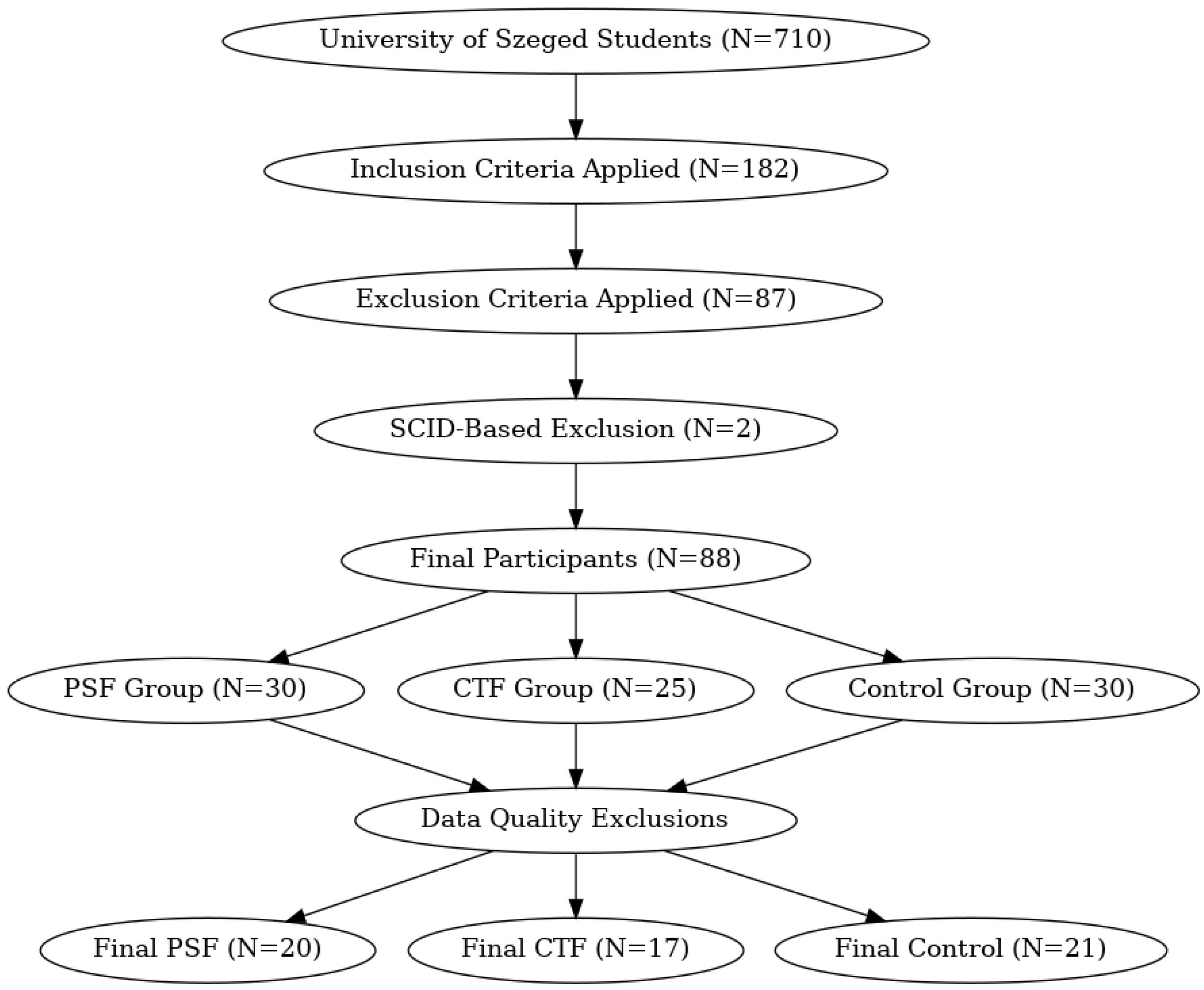
| Initial Inclusion | University of Szeged first- and second-year students without a diagnosed psychiatric disorder. |
| Screening Questionnaires | TEMPS-A (Temperament), O-LIFE (Schizotypy), PDI-21 (Delusions), MDQ (Mood Disorder). |
| Inclusion Criteria | 182 students met the screening criteria. |
| Exclusion Criteria | 87 students excluded based on criteria, additional 2 excluded due to acute mental disorders (SCID-5). |
| Final Grouping | PSF Group: O-LIFE ≥ 5, PDI-21 > 10, TEMPS-A Cyclothymia < 12 (N = 30). CTF Group: O-LIFE < 6, TEMPS-A Cyclothymia total score = 11 (N = 25). Control Group: No significant psychopathology (N = 30). |
| Data Quality Control | Removal of participants with excessively noisy or impaired EEG data. |
| Final Sample Size | PSF: N = 20 (12 men, 8 women), mean age 27.66 (SD = 1.75). CTF: N = 17 (6 men, 11 women), mean age 26.82 (SD = 1.85). Control: N = 21 (9 men, 12 women), mean age 27.45 (SD = 1.89). |
| C-CTF | C-PSF | CTF-PSF | |
|---|---|---|---|
| ANN (AHFS) | 0.89 | 0.92 | 0.91 |
| ANN (CFFS) | 0.79 | 0.71 | 0.62 |
| LR | 0.76 | 0.71 | 0.65 |
| RF | 0.79 | 0.80 | 0.65 |
| CP5 | AF4 | F8 | Fp1 | CP1 | FC5 | O2 | P4 |
| L. BA39 | R. BA9 | R. BA45 | L. BA10 | L. BA7 | L. BA6 | R. BA18 | R. BA39 |
| PO3 | Cz | PO4 | AF3 | C4 | CP2 | FC2 | O1 |
| L. BA19 | R. BA4 | R. BA19 | L. BA9 | R. BA1 | R. BA7 | R. BA6 | L. BA18 |
| CP5 | FC5 | CP6 | T7 | Fp1 | P7 | CP6 | C4 |
| L. BA39 | L. BA6 | R. BA39 | L. BA21 | L. BA10 | L. BA19 | R. BA39 | R. BA1 |
| FC2 | F8 | Cz | Fz | AF3 | P8 | PO3 | P4 |
| R. BA6 | R. BA45 | R. BA4 | L. BA6 | L. BA9 | R. BA19 | L. BA19 | R. BA39 |
| CP1 | FC1 | C3 | |||||
| L. BA7 | L. BA6 | L. BA1 |
| Key Findings | PSF Group | CTF Group | Brain Regions (Brodmann Areas) | Literature & Observations |
|---|---|---|---|---|
| Gamma Frequency | Features of CP5 channel | Features of CP5 channel | BA39 (Angular Gyrus) | Gamma waves linked to high-order cognitive functions [36]. |
| Lempel-Ziv Complexity | - | Feature of FC5 channel | BA6 (Supplementary motor area) | LZC reduction in SZ suggests impaired neural adaptability [54]. Based on our findings, it may also be relevant in BD. |
| PSF-CTF differentiation | Features of PO4 and P4 channels | Features of PO4 and P4 channels | BA19, BA39 | Angular gyrus role in cognitive differences between schizophrenia and bipolar disorder [9]. |
Disclaimer/Publisher’s Note: The statements, opinions and data contained in all publications are solely those of the individual author(s) and contributor(s) and not of MDPI and/or the editor(s). MDPI and/or the editor(s) disclaim responsibility for any injury to people or property resulting from any ideas, methods, instructions or products referred to in the content. |
© 2025 by the authors. Licensee MDPI, Basel, Switzerland. This article is an open access article distributed under the terms and conditions of the Creative Commons Attribution (CC BY) license (https://creativecommons.org/licenses/by/4.0/).
Share and Cite
Gubics, F.; Nagy, Á.; Dombi, J.; Pálfi, A.; Szabó, Z.; Viharos, Z.J.; Hoang, A.T.; Bilicki, V.; Szendi, I. A Machine-Learning-Based Analysis of Resting State Electroencephalogram Signals to Identify Latent Schizotypal and Bipolar Development in Healthy University Students. Diagnostics 2025, 15, 454. https://doi.org/10.3390/diagnostics15040454
Gubics F, Nagy Á, Dombi J, Pálfi A, Szabó Z, Viharos ZJ, Hoang AT, Bilicki V, Szendi I. A Machine-Learning-Based Analysis of Resting State Electroencephalogram Signals to Identify Latent Schizotypal and Bipolar Development in Healthy University Students. Diagnostics. 2025; 15(4):454. https://doi.org/10.3390/diagnostics15040454
Chicago/Turabian StyleGubics, Flórián, Ádám Nagy, József Dombi, Antónia Pálfi, Zoltán Szabó, Zsolt János Viharos, Anh Tuan Hoang, Vilmos Bilicki, and István Szendi. 2025. "A Machine-Learning-Based Analysis of Resting State Electroencephalogram Signals to Identify Latent Schizotypal and Bipolar Development in Healthy University Students" Diagnostics 15, no. 4: 454. https://doi.org/10.3390/diagnostics15040454
APA StyleGubics, F., Nagy, Á., Dombi, J., Pálfi, A., Szabó, Z., Viharos, Z. J., Hoang, A. T., Bilicki, V., & Szendi, I. (2025). A Machine-Learning-Based Analysis of Resting State Electroencephalogram Signals to Identify Latent Schizotypal and Bipolar Development in Healthy University Students. Diagnostics, 15(4), 454. https://doi.org/10.3390/diagnostics15040454