
Connectogram-COH: A Coherence-Based Time-Graph Representation for EEG-Based Alzheimer’s Disease Detection


Abstract
1. Introduction
2. Data and Methodology
2.1. Dataset
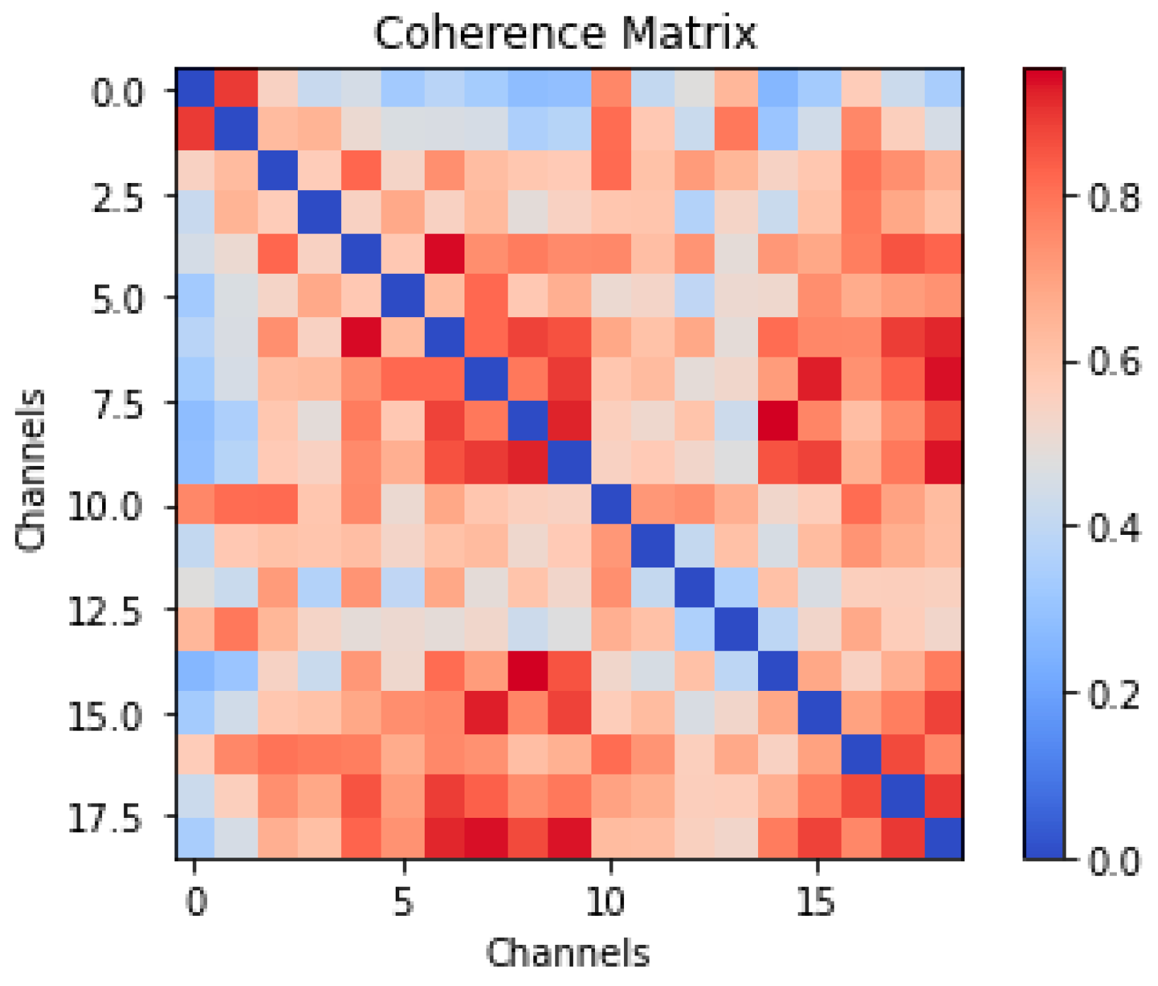
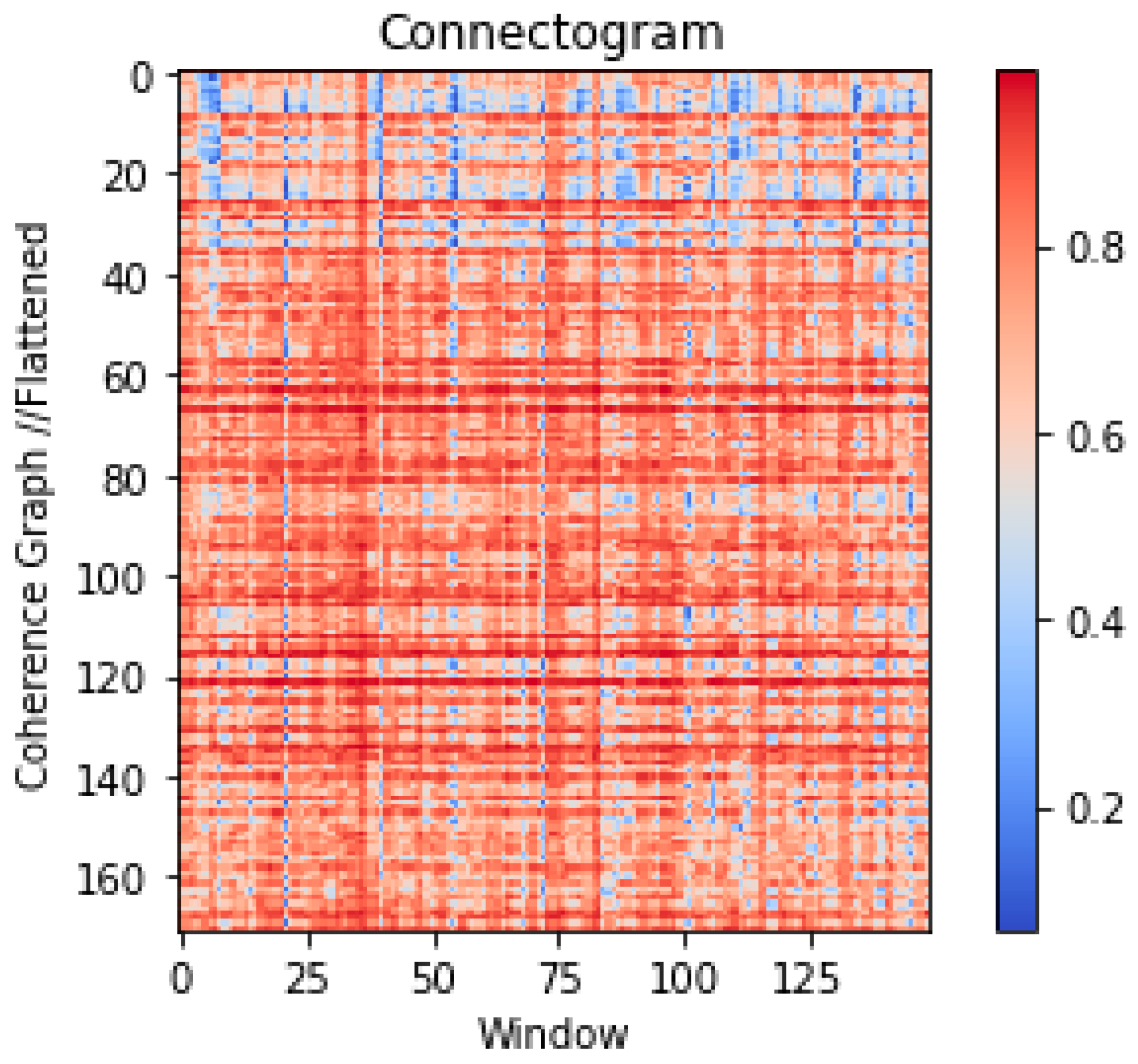
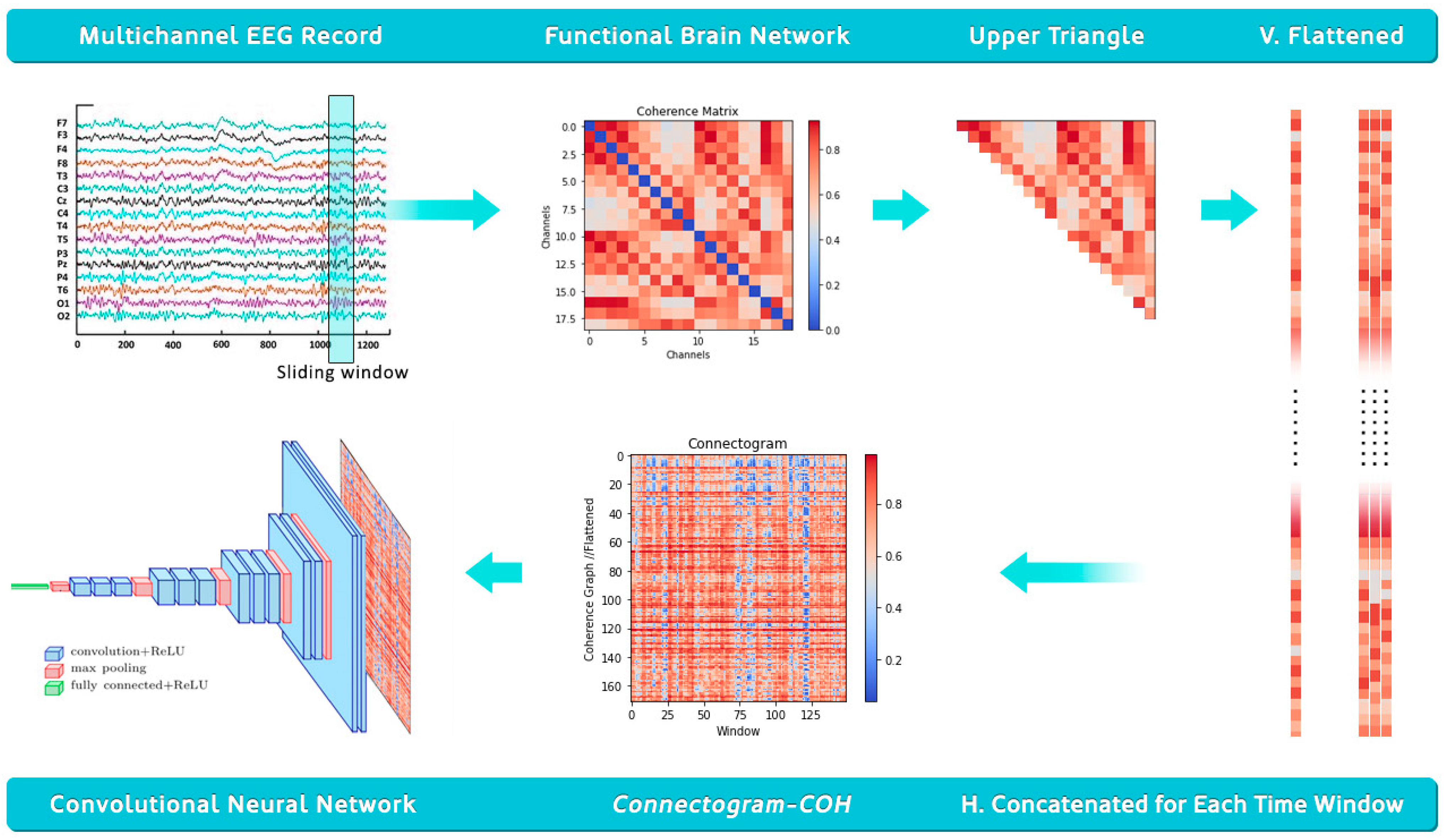
2.2. Data Processing for Time Graph Conversion
2.3. Experimental Setup
2.3.1. Convolutional Neural Network (CNN)
2.3.2. Residual Network (ResNet)
2.3.3. VGG-16
2.3.4. Inception v3
2.3.5. EfficientNet-B7
2.3.6. DenseNet-121
3. Results and Discussion
4. Model Deployment
5. Limitations and Future Directions
- Fixed Electrode Count: The current design supports only 19-channel EEG. For high-density arrays, the image size may become unwieldy. Future work could use graph pooling, dimensionality reduction, or adaptive montages to scale effectively.
- Aspect Ratio Issues: Some CNN models (e.g., InceptionV3, EfficientNetB7) struggle with the elongated shape of connectograms. Padding, resizing, or using models that accept non-square inputs can improve compatibility.
- Explainability: Explainable AI (XAI) techniques applied to Connectogram-COH images to highlight which regions most influence the model’s predictions would give valuable insights to the study. Additionally, for EEG coherence graphs, graph-specific explainability approaches could offer insight into which connections or brain regions are most critical to the classification. These additions would help clinicians to better understand and trust the model’s decisions, and we view them as a vital direction for future work.
- Implement dynamic window sizing and normalization to better handle varying EEG lengths, sampling rates, and channel counts.
- Benchmark the method on multiple public datasets, using fine-tuning or domain adaptation as needed.
- Explore graph-based models (such as GNN) to retain spatial and temporal structures for improved performance.
- Apply transfer learning to adapt pretrained models to smaller, clinical datasets.
6. Conclusions
Author Contributions
Funding
Institutional Review Board Statement
Informed Consent Statement
Data Availability Statement
Conflicts of Interest
References
- Puri, D.V.; Nalbalwar, S.L.; Nandgaonkar, A.B.; Gawande, J.P.; Wagh, A. Automatic detection of Alzheimer’s disease from EEG signals using low-complexity orthogonal wavelet filter banks. Biomed. Signal Process. Control 2023, 81, 104439. [Google Scholar] [CrossRef]
- Fernández, M.; Gobartt, A.L.; Balañá, M. Behavioural symptoms in patients with Alzheimer’s disease and their association with cognitive impairment. BMC Neurol. 2010, 10, 87. [Google Scholar] [CrossRef] [PubMed]
- Atri, A. The Alzheimer’s disease clinical spectrum. Med. Clin. N. Am. 2019, 103, 263–293. [Google Scholar] [CrossRef] [PubMed]
- Ding, Y.; Chu, Y.; Liu, M.; Ling, Z.; Wang, S.; Li, X.; Li, Y. Fully automated discrimination of Alzheimer’s disease using resting-state electroencephalography signals. Quant. Imaging Med. Surg. 2022, 12, 1063–1078. [Google Scholar] [CrossRef]
- Dubois, B. Research criteria for the diagnosis of Alzheimer’s disease: Revising the NINCDS-ADRDA criteria. Lancet Neurol. 2007, 6, 734–746. [Google Scholar] [CrossRef]
- Miltiadous, A.; Tzimourta, K.D.; Giannakeas, N.; Tsipouras, M.G.; Glavas, E.; Kalafatakis, K.; Tzallas, A.T. Machine learning algorithms for epilepsy detection based on published EEG databases: A systematic review. IEEE Access 2023, 11, 564–594. [Google Scholar] [CrossRef]
- Geraedts, V.J.; Boon, L.I.; Marinus, J.; Gouw, A.A.; van Hilten, J.J.; Stam, C.J.; Tannemaat, M.R.; Contarino, M.F. Clinical correlates of quantitative EEG in Parkinson disease. Neurology 2018, 91, 871–883. [Google Scholar] [CrossRef]
- Alhassan, S.; Soudani, A. Energy-aware EEG-based Scheme for early-age Autism detection. In Proceedings of the 2022 2nd International Conference of Smart Systems and Emerging Technologies (SMARTTECH), Riyadh, Saudi Arabia, 9–11 May 2022; IEEE: New York, NY, USA, 2022; pp. 97–102. [Google Scholar]
- Kulkarni, N.N.; Bairagi, V.K. Extracting salient features for EEG-based diagnosis of Alzheimer’s disease using support vector machine classifier. IETE J. Res. 2017, 63, 11–22. [Google Scholar] [CrossRef]
- Miltiadous, A.; Gionanidis, E.; Tzimourta, K.D.; Giannakeas, N.; Tzallas, A.T. DICE-Net: A Novel Convolution-Transformer Architecture for Alzheimer Detection in EEG Signals. IEEE Access 2023, 11, 71840–71858. [Google Scholar] [CrossRef]
- Safi, M.S.; Safi, S.M.M. Early detection of Alzheimer’s disease from EEG signals using Hjorth parameters. Biomed. Signal Process. Control 2021, 65, 102338. [Google Scholar] [CrossRef]
- Şeker, M.; Özbek, Y.; Yener, G.; Özerdem, M.S. Complexity of EEG dynamics for early diagnosis of Alzheimer’s disease using permutation entropy neuromarker. Comput. Methods Programs Biomed. 2021, 206, 106116. [Google Scholar] [CrossRef] [PubMed]
- Tzimourta, K.D.; Giannakeas, N.; Tzallas, A.T.; Astrakas, L.G.; Afrantou, T.; Ioannidis, P.; Grigoriadis, N.; Angelidis, P.; Tsalikakis, D.G.; Tsipouras, M.G. EEG window length evaluation for the detection of Alzheimer’s disease over different brain regions. Brain Sci. 2019, 9, 81. [Google Scholar] [CrossRef] [PubMed]
- Roy, Y.; Banville, H.; Albuquerque, I.; Gramfort, A.; Falk, T.H.; Faubert, J. Deep learning-based electroencephalography analysis: A systematic review. J. Neural Eng. 2019, 16, 051001. [Google Scholar] [CrossRef] [PubMed]
- Olgun, N.; Özkaynak, E. Complex Network Analysis of EEG Signals of Epilepsy Patients. In Proceedings of the 32nd Signal Processing and Communications Applications Conference (SIU), Mersin, Turkey, 15–18 May 2024; pp. 1–4. [Google Scholar] [CrossRef]
- Olgun, N.; Özkaynak, E. A novel approach to detecting epileptic patients: Complex network-based EEG classification. J. Complex Netw. 2024, 12, cnae044. [Google Scholar] [CrossRef]
- Zhang, D.; Yin, J.; Zhu, X.; Zhang, C. Network representation learning: A survey. IEEE Trans. Big Data 2020, 6, 3–28. [Google Scholar] [CrossRef]
- Bastos, A.M.; Schoffelen, J.M. Investigation of functional connectivity using MEG: Assessing the influence of source modeling approaches. NeuroImage 2016, 186, 370–380. [Google Scholar] [CrossRef]
- Kabbara, A.; El Falou, R.; Khalil, C.; Hassan, M. Scalp-EEG Network-Based Analysis of AD. arXiv 2017, arXiv:1706.03839. [Google Scholar]
- Wang, Y.; Zhang, J.; Chen, L.; Wang, S. LEAD: A Large Foundation Model for EEG-Based Alzheimer’s Disease Detection. arXiv 2025, arXiv:2502.01678. [Google Scholar]
- Stam, C.J. Modern network science of cognitive dynamics: A review. Neurosci. Biobehav. Rev. 2014, 48, 32–42. [Google Scholar]
- Gollo, L.L.; Breakspear, M. The human connectome: A structural description of the human brain network. Brain Cogn. 2014, 88, 95–109. [Google Scholar]
- Alves, C.L.; Vigário, R.; Rodrigues, P.M. EEG Functional Connectivity and Deep Learning for Automatic Diagnosis. arXiv 2021, arXiv:2110.06140. [Google Scholar]
- Demir, A.; Ertam, F.; Cetin, A.E. EEG-GNN: Graph Neural Networks for EEG Classification. arXiv 2021, arXiv:2106.09135. [Google Scholar]
- Gupta, T.; Zhang, W.; Wu, D. Tensor Decomposition of Large-Scale EEGs. arXiv 2022, arXiv:2211.13793. [Google Scholar]
- Wang, Y.; Zhang, J.; Chen, L.; Wang, S. Flexible and Explainable Graph Analysis for EEG-Based Alzheimer’s. arXiv 2025, arXiv:2504.01329. [Google Scholar]
- Ajra, Z.; Belkacem, S.; El Khiat, H.; El Ansari, M. Shallow Neural Networks With Functional Connectivity. Front. Neurol. 2023, 14, 1270405. [Google Scholar] [CrossRef]
- Fruehwirt, W.; Steinheimer, J.M.; Scherer, R. Bayesian DNNs for AD Severity Estimation. arXiv 2018, arXiv:1812.04994. [Google Scholar]
- Ranjan, S.; Jaiswal, S.; Kumar, R. Subcortical EEG-Based AD and FTD Classification. arXiv 2024, arXiv:2408.10816. [Google Scholar]
- Sunkara, A.; Chandak, S.; Varshney, P.K. ANNs vs. KANs in EEG Alzheimer Detection. arXiv 2024, arXiv:2409.05989. [Google Scholar]
- Sharma, N.; Kolekar, M.H.; Jha, K. EEG based dementia diagnosis using multi-class support vector machine with motor speed cognitive test. Biomed. Signal Process. Control 2021, 63, 102102. [Google Scholar] [CrossRef]
- Praveena, D.M.; Sarah, D.A.; George, S.T. Deep learning techniques for EEG signal applications—A review. IETE J. Res. 2022, 68, 3030–3037. [Google Scholar] [CrossRef]
- Miltiadous, A. A dataset of 88 EEG recordings from: Alzheimer’s disease, Frontotemporal dementia and healthy subjects. OpenNeuro 2023, 1, ds004504. [Google Scholar] [CrossRef]
- Miltiadous, A.; Tzimourta, K.D.; Afrantou, T.; Ioannidis, P.; Grigoriadis, N.; Tsalikakis, D.G.; Angelidis, P.; Tsipouras, M.G.; Glavas, E.; Giannakeas, N.; et al. A dataset of scalp EEG recordings of Alzheimer’s disease, frontotemporal dementia and healthy subjects from routine EEG. Data 2023, 8, 95. [Google Scholar] [CrossRef]
- Türker, I.; Aksu, S. Connectogram—A graph-based time dependent representation for sounds. Appl. Acoust. 2022, 191, 108660. [Google Scholar] [CrossRef]
- Sarwinda, D.; Paradisa, R.H.; Bustamam, A.; Anggia, P. Deep Learning in Image Classification using Residual Network (ResNet) Variants for Detection of Colorectal Cancer. Procedia Comput. Sci. 2021, 179, 423–431. Available online: https://www.sciencedirect.com/science/article/pii/S1877050921000284 (accessed on 1 December 2024). [CrossRef]
- Eskandari, S.; Eslamian, A.; Munia, N.; Alqarni, A.; Cheng, Q. Evaluating Deep Learning Models for Breast Cancer Classification: A Comparative Study. arXiv 2025, arXiv:2408.16859v2. Available online: https://arxiv.org/pdf/2408.16859 (accessed on 1 December 2024). [Google Scholar]
- Ozdenizci, O.; Eldeeb, S.; Demir, A.; Erdoğmuş, D.; Akçakaya, M. EEG-based texture roughness classification in active tactile exploration with invariant representation learning networks. Biomed. Signal Process. Control 2021, 67, 102507. [Google Scholar] [CrossRef]
- Seo, J.; Laine, T.H.; Oh, G.; Sohn, K.A. EEG-based emotion classification for Alzheimer’s disease patients using conventional machine learning and recurrent neural network models. Sensors 2020, 20, 7212. [Google Scholar] [CrossRef]
- Dogan, S.; Baygin, M.; Tasci, B.; Loh, H.W.; Barua, P.D.; Tuncer, T.; Tan, R.-S.; Acharya, U.R. Primate brain pattern-based automated Alzheimer’s disease detection model using EEG signals. Cogn. Neurodynamics 2022, 17, 647–659. [Google Scholar] [CrossRef]
- Miltiadous, A.; Tzimourta, K.D.; Giannakeas, N.; Tsipouras, M.G.; Afrantou, T.; Ioannidis, P.; Tzallas, A.T. Alzheimer’s disease and frontotemporal dementia: A robust classification method of EEG signals and a comparison of validation methods. Diagnostics 2021, 11, 1437. [Google Scholar] [CrossRef]
- Araujo, T.; Teixeira, J.P.; Rodrigues, P.M. Smart-data-driven system for Alzheimer disease detection through electroencephalographic signals. Bioengineering 2022, 9, 141. [Google Scholar] [CrossRef]
- Gomez, S.R.; Gomez, C.; Poza, J.; Tobal, G.G.; Arribas, M.T.; Cano, M.; Hornero, R. Automated multiclass classification of spontaneous EEG activity in Alzheimer’s disease and mild cognitive impairment. Entropy 2018, 20, 35. [Google Scholar] [CrossRef] [PubMed]
- Khatun, S.; Morshed, B.I.; Bidelman, G.M. A single-channel EEG-based approach to detect mild cognitive impairment via speech-evoked brain responses. IEEE Trans. Neural Syst. Rehabil. Eng. 2019, 27, 1063–1070. [Google Scholar] [CrossRef] [PubMed]
- Gordon, E.; Rohrer, J.D.; Kim, L.G.; Omar, R.; Rossor, M.N.; Fox, N.C.; Warren, J.D. Measuring disease progression in frontotemporal lobar degeneration: A clinical and MRI study. Neurology 2010, 74, 666–673. [Google Scholar] [CrossRef] [PubMed]
- Lopes, M.; Cassani, R.; Falk, T.H. Using CNN saliency maps and EEG modulation spectra for improved and more interpretable machine learning-based Alzheimer’s disease diagnosis. Comput. Intell. Neurosci. 2023, 2023, 3198066. [Google Scholar] [CrossRef]
- Ieracitano, C.; Mammone, N.; Bramanti, A.; Hussain, A.; Morabito, F.C. A Convolutional Neural Network approach for classification of dementia stages based on 2D-spectral representation of EEG recordings. Neurocomputing 2019, 323, 96–107. [Google Scholar] [CrossRef]
- Xia, W.; Zhang, R.; Zhang, X.; Usman, M. A novel method for diagnosing Alzheimer’s disease using deep pyramid CNN based on EEG signals. Heliyon 2023, 9, e14858. [Google Scholar] [CrossRef]
- Xiaojun, B.; Haibo, W. Early Alzheimer’s disease diagnosis based on EEG spectral images using deep learning. Neural Netw. 2019, 114, 119–135. [Google Scholar]
- Siuly, S.; Alçin, Ö.F.; Kabir, E.; Sengür, A.; Wang, H.; Zhang, Y.; Whittaker, F. A New Framework for Automatic Detection of Patients With Mild Cognitive Impairment Using Resting-State EEG Signals. IEEE Trans. Neural Syst. Rehabil. Eng. 2020, 28, 1966–1976. [Google Scholar] [CrossRef]
- Ismail, M.; Hofmann, K.; Abd El Ghany, M.A. Early diagnoses of Alzheimer using EEG data and deep neural networks classification. In Proceedings of the 2019 IEEE Global Conference on Internet of Things (GCIoT), Dubai, United Arab Emirates, 4–7 December 2019. [Google Scholar] [CrossRef]
- Wen, D.; Zhou, Y.; Li, P.; Zhang, P.; Li, J.; Wang, Y.; Li, X.; Bian, Z.; Yin, S.; Xu, Y. Resting-state EEG signal classification of amnestic mild cognitive impairment with type 2 diabetes mellitus based on multispectral image and convolutional neural network. J. Neural Eng. 2020, 17, 036005. [Google Scholar] [CrossRef]
- Cassani, R.; Falk, T.H. Alzheimer’s Disease Diagnosis and Severity Level Detection Based on Electroencephalography Modulation Spectral ‘Patch’ Features. IEEE J. Biomed. Health Inform. 2020, 24, 1982–1993. [Google Scholar] [CrossRef]
- Huggins, C.J.; Escudero, J.; Parra, M.A.; Scally, B.; Anghinah, R.; De Arajujo, A.V.L.; Basile, L.F.; Abasolo, D. Deep learning of resting-state electroencephalogram signals for three-class classification of Alzheimer’s disease, mild cognitive impairment and healthy ageing. J. Neural Eng. 2021, 18, 046087. [Google Scholar] [CrossRef] [PubMed]
- Amini, M.; Pedram, M.M.; Moradi, A.R.; Ouchani, M. Diagnosis of Alzheimer’s Disease by Time-Dependent Power Spectrum Descriptors and Convolutional Neural Network Using EEG Signal. Comput. Math. Methods Med. 2021, 2021, 5511922. [Google Scholar] [CrossRef] [PubMed]
- Wu, L.; Zhao, Q.; Liu, J.; Yu, H. Efficient identification of Alzheimer’s brain dynamics with Spatial-Temporal Autoencoder: A deep learning approach for diagnosing brain disorders. Biomed. Signal Process. Control 2023, 86, 104917. [Google Scholar] [CrossRef]
- Zhou, H.; Yin, L.; Su, R.; Zhang, Y.; Yuan, Y.; Xie, P.; Li, X. STCGRU: A hybrid model based on CNN and BiGRU for mild cognitive impairment diagnosis. Comput. Methods Programs Biomed. 2024, 248, 108123. [Google Scholar] [CrossRef]
- Parra, C.R.; Torres, A.P.; Reolid, R.S.; Sotos, J.M.; Borjab, A.L. Inter-hospital moderate and advanced Alzheimer’s disease detection through convolutional neural networks. Heliyon 2024, 10, e26298. [Google Scholar] [CrossRef]


| Layer | Type | Output Shape | Details |
|---|---|---|---|
| Input | Input Layer | (None, 171, 149, 1) | - |
| Conv2D | Convolutional Layer | (None, 169, 147, 32) | Filters: 32, Kernel: 3, Stride: 1 |
| MaxPooling2D | Pooling Layer | (None, 84, 73, 32) | Pool Size: 2 |
| Conv2D | Convolutional Layer | (None, 82, 71, 64) | Filters: 64, Kernel: 3, Stride: 1 |
| MaxPooling2D | Pooling Layer | (None, 41, 35, 64) | Pool Size: 2 |
| Conv2D | Convolutional Layer | (None, 39, 33, 128) | Filters: 128, Kernel: 3, Stride: 1 |
| MaxPooling2D | Pooling Layer | (None, 19, 16, 128) | Pool Size: 2 |
| Flatten | Flatten Layer | (None, 38,912) | - |
| Dense | Fully Connected Layer | (None, 128) | Units: 128 |
| Dense | Fully Connected Layer | (None, 3) | Units: 3 (Output classes) |
| Layer | Type | Output Shape | Details |
|---|---|---|---|
| Input | Input Layer | (None, 171, 149) | - |
| Conv1D | Convolutional Layer | (None, 86, 64) | Filters: 64, Kernel: 3, Stride: 2 |
| BatchNorm | Batch Normalization | (None, 86, 64) | - |
| Activation | ReLU Activation | (None, 86, 64) | - |
| MaxPooling1D | Pooling Layer | (None, 43, 64) | Pool Size: 2 |
| Residual Block 1 | 2x Conv + Add | (None, 43, 64) | Skip connection, Filters: 64, Kernel: 3 |
| Residual Block 2 | 2x Conv + Add | (None, 22, 128) | Strided conv for downsampling, Filters: 128 |
| Residual Block 3 | 2x Conv + Add | (None, 11, 256) | Strided conv for downsampling, Filters: 256 |
| GlobalAvgPooling | Global Avg Pooling | (None, 256) | - |
| Dense | Fully Connected Layer | (None, 3) | Units: 3 (Output classes) |
| Model/Segment Len. | 30 s | 20 s | 10 s |
|---|---|---|---|
| CNN | 96.28 | 97.82 | 98.63 |
| ResNet | 98.59 | 99.09 | 99.49 |
| VVG 16 | 77.68 | 73.04 | 73.55 |
| InceptionV3 | 71.33 | N/A | N/A |
| EfficientNetB7 | 41.79 | 41.73 | 41.71 |
| DenseNet121 | 69.36 | 69.42 | N/A |
| Accuracy | Precision | Recall | F1-Score | Support | ||
|---|---|---|---|---|---|---|
| ResNet | CN | 0.9859 | 0.9875 | 0.9875 | 0.9875 | 158 |
| AD | 0.9859 | 0.9843 | 0.9741 | 0.9792 | 191 | |
| FTD | 0.9859 | 0.9623 | 0.9808 | 0.9714 | 108 | |
| CNN | CN | 0.9672 | 0.9625 | 0.9747 | 0.9686 | 158 |
| AD | 0.9672 | 0.9737 | 0.9686 | 0.9711 | 191 | |
| FTD | 0.9672 | 0.9626 | 0.9537 | 0.9581 | 108 | |
| VVG16 | CN | 0.7877 | 0.7268 | 0.8924 | 0.8011 | 158 |
| AD | 0.7877 | 0.8471 | 0.7539 | 0.7978 | 191 | |
| FTD | 0.7877 | 0.8065 | 0.6944 | 0.7463 | 108 | |
| InceptionV3 | CN | 0.7155 | 0.7143 | 0.7278 | 0.7210 | 158 |
| AD | 0.7155 | 0.7404 | 0.8063 | 0.7719 | 191 | |
| FTD | 0.7155 | 0.6591 | 0.5370 | 0.5918 | 108 | |
| EfficientNetB7 | CN | 0.4179 | 0.0000 | 0.0000 | 0.0000 | 158 |
| AD | 0.4179 | 0.4179 | 1.0000 | 0.5895 | 191 | |
| FTD | 0.4179 | 0.0000 | 0.0000 | 0.0000 | 108 | |
| DenseNet121 | CN | 0.6980 | 0.7066 | 0.7468 | 0.7262 | 158 |
| AD | 0.6980 | 0.7198 | 0.6859 | 0.7024 | 191 | |
| FTD | 0.6980 | 0.6481 | 0.6481 | 0.6481 | 108 |
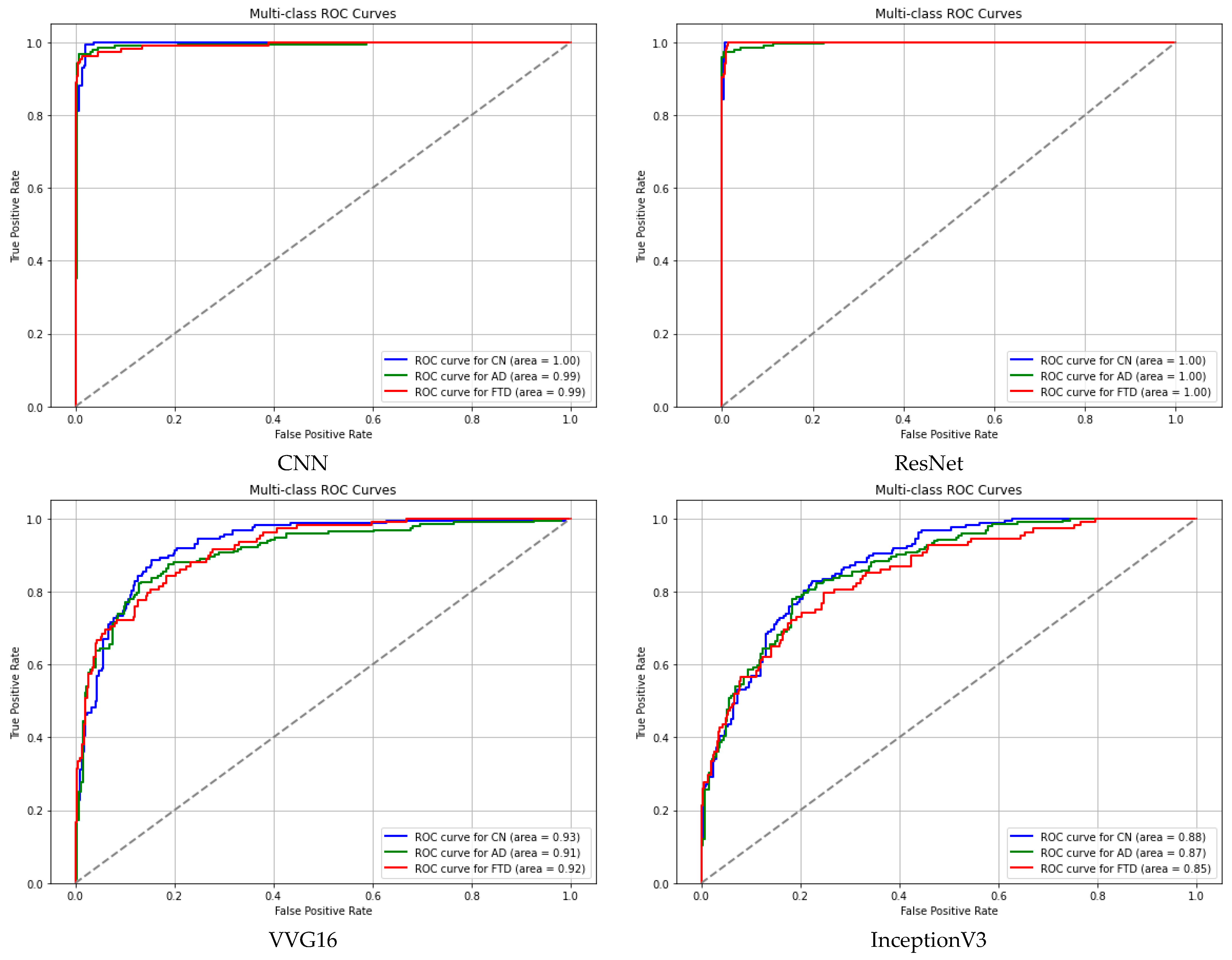
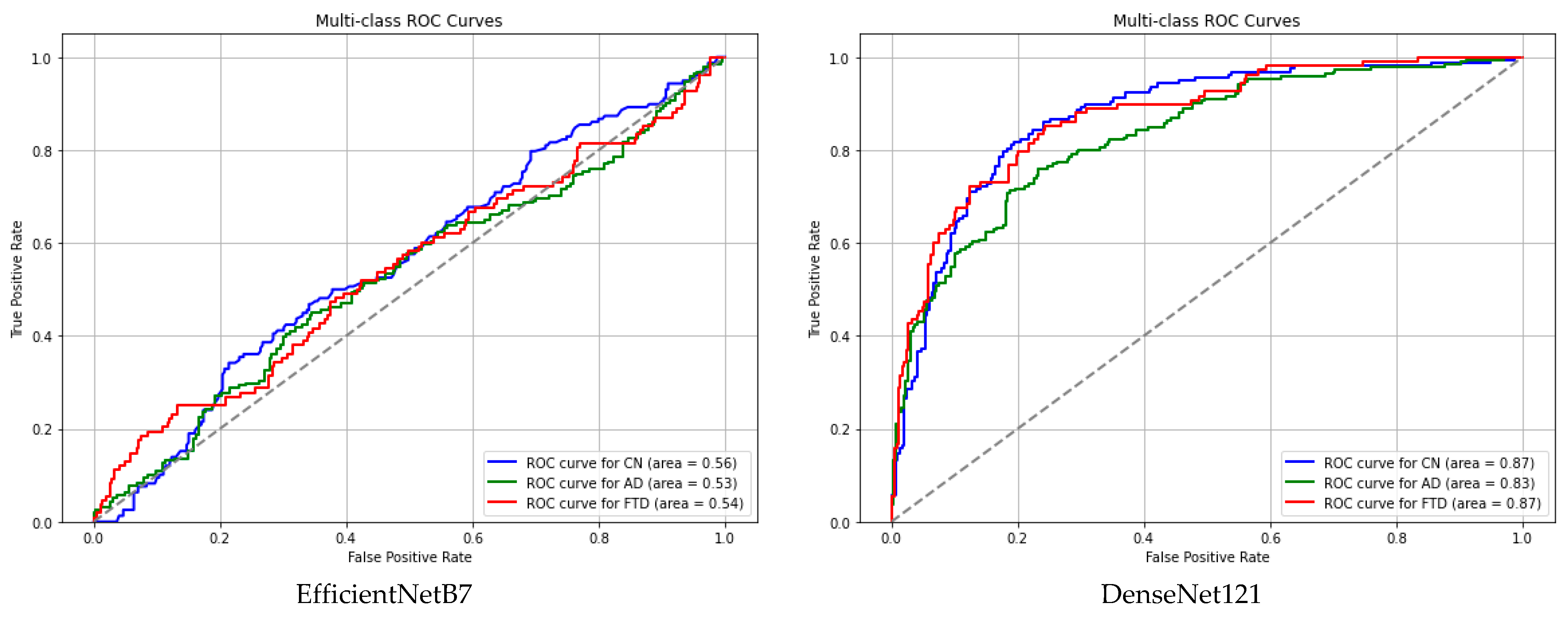
| CN | AD | FTD | |
|---|---|---|---|
| ResNet | 0.9995 | 0.9989 | 0.9999 |
| CNN | 0.9963 | 0.9924 | 0.9934 |
| VVG16 | 0.9253 | 0.9066 | 0.9160 |
| InceptionV3 | 0.8757 | 0.8658 | 0.8489 |
| EfficientNetB7 | 0.5593 | 0.5288 | 0.5429 |
| DenseNet121 | 0.8716 | 0.8320 | 0.8726 |
| Epochs\Batch_Size | 4 | 8 | 16 | 32 | 64 | 128 | 256 | 512 | |
|---|---|---|---|---|---|---|---|---|---|
| 10 s segments | 20 | 98.77 | 99.49 | 98.99 | 98.41 | 97.62 | 97.47 | 94.52 | 71.54 |
| 50 | 99.63 | 99.42 | 99.06 | 99.49 | 99.49 | 98.41 | 95.24 | 88.61 | |
| 70 | 99.35 | 99.27 | 99.27 | 99.49 | 99.56 | 99.42 | 96.58 | 89.21 | |
| 100 | 99.42 | 99.27 | 99.20 | 99.49 | 99.63 | 98.99 | 97.81 | 91.18 | |
| 20 s segments | 20 | 93.18 | 95.94 | 97.82 | 98.63 | 99.27 | 89.27 | 71.15 | 50.28 |
| 50 | 99.42 | 99.42 | 98.40 | 98.82 | 98.84 | 97.24 | 89.19 | 70.43 | |
| 70 | 99.13 | 99.27 | 98.98 | 99.27 | 99.42 | 98.81 | 89.27 | 79.56 | |
| 100 | 98.26 | 99.56 | 99.42 | 98.99 | 97.39 | 95.79 | 89.56 | 77.82 | |
| 30 s segments | 20 | 96.49 | 98.90 | 98.03 | 98.03 | 93.93 | 81.16 | 62.45 | 58.29 |
| 50 | 97.37 | 97.59 | 98.24 | 97.81 | 98.03 | 95.18 | 89.27 | 70.32 | |
| 70 | 98.03 | 97.59 | 98.03 | 98.24 | 98.24 | 96.14 | 87.23 | 71.33 | |
| 100 | 98.90 | 98.86 | 98.41 | 98.41 | 98.59 | 94.21 | 88.55 | 71.99 |
| Author(s) | Year | Classifier | Size of the Dataset | No. of Channels | Segment Length (s) | Folds for CV | Accuracy |
|---|---|---|---|---|---|---|---|
| Gomez et al. [43] | 2018 | MLP | 111 | 19 | - | - | AD-MCI-CN: 78.43 |
| Xiaojun & Haibo [49] | 2019 | CNN | 12 | 64 | - | 1–10 | 95.04 |
| Ieracitano et al. [47] | 2019 | CNN | 189 | 19 | 5 | 8 | AD-CN: 92.95 AD-MCI: 84.61 MCI-CN: 91.88 AD-MCI-CN: 83.33 |
| Khatun et al. [44] | 2019 | ERP SVM | 23 | 1 | - | - | 87.9 |
| Ismail et al. [51] | 2019 | CNN | 60 | 10 | 16 | - | AD-CN: 92.52 MCI-CN: 90.36 |
| Wen et al. [52] | 2020 | CNN | 39 | 19 | - | 5 | 92.92 |
| Siluy et al. [50] | 2020 | ELM SVM KNN | 27 | 19 | 2 | 10 | ELM: 98.78 SVM: 97.41 KNN: 98.19 |
| Cassani et al. [53] | 2020 | SVM | 54 | 20 | 8 | - | 78.7 |
| Safi & Safi [11] | 2021 | SVM KNN RLDA | 86 | 20 | 8 | - | SVM: 95.79 KNN: 97.64 RLDA: 97.02 |
| Miltiadous et al. [41] | 2021 | Meny | 28 | 19 | 5 | 10 | AD-CN: 78.58 FTD-CN: 86.30 |
| Huggins et al. [54] | 2021 | CNN | 141 | 20 | 5 | 10 | 99.3 AD 98.3 MCI 98.8 CN |
| Amini et al. [55] | 2021 | CNN | 192 | 19 | - | - | 82.3 |
| Dogan et al. [40] | 2022 | KNN | 23 | 16 | - | 10 | 92.1 |
| Araujo et al. [42] | 2022 | SVM | 38 | 19 | 5 | - | AD-CN: 81 MCI-CN: 79 |
| Ding et al. [4] | 2022 | Meny | 301 | 60 | 15 | 5 | AD-CN: 72.43 AD-MCI: 69.11 MCI-CN: 59.91 |
| Xia et al. [48] | 2023 | CNN | 100 | 19 | - | 5 | AD-MCI-CN: 97.10 |
| Wu et al. [56] | 2023 | STAE | 53 | 16 | 1 | - | 96.30 |
| Lopes et al. [46] | 2023 | CNN SVM | 54 | 20 | 8 | - | 87.3 |
| Miltiadous et al. [10] | 2023 | DICE-net | 88 | 19 | 30 | 5 | AD-CN: 83.28 FTD-CN: 74.96 |
| Zhou et al. [57] | 2024 | STCGRU | 27 | 19 | 5 | 10 | MCI: 99.95 |
| Parra et al. [58] | 2024 | CNN | 668 | 32 | - | 5 | CN-ADA: 97.49 CN-ADM: 97.03 |
| Our study | 2024 | ResNet | 88 | 19ch | 30 20 10 | 5 | AD-CN: 99.53 AD-FTD: 99.45 FTD-CN: 99.50 AD-FTD-CN: 99.41 |
| Metric | Value | Comment |
|---|---|---|
| Trainable Parameters | 979,715 | Medium-sized model. Can run on desktop, mid-level mobile, or embedded edge devices. |
| Model Size | 11.45 MB | Compact enough for mobile apps or cloud API deployment. |
| Inference Latency | 147.4 ms (1 sample) | Good for near real-time processing, but may need optimization for ultra low-latency apps (e.g., BCI, live EEG). |
| Throughput | 234.4 samples/s | Very efficient batch processing—good for offline or background inference. |
Disclaimer/Publisher’s Note: The statements, opinions and data contained in all publications are solely those of the individual author(s) and contributor(s) and not of MDPI and/or the editor(s). MDPI and/or the editor(s) disclaim responsibility for any injury to people or property resulting from any ideas, methods, instructions or products referred to in the content. |
© 2025 by the authors. Licensee MDPI, Basel, Switzerland. This article is an open access article distributed under the terms and conditions of the Creative Commons Attribution (CC BY) license (https://creativecommons.org/licenses/by/4.0/).
Share and Cite
Aljanabi, E.; Türker, İ. Connectogram-COH: A Coherence-Based Time-Graph Representation for EEG-Based Alzheimer’s Disease Detection. Diagnostics 2025, 15, 1441. https://doi.org/10.3390/diagnostics15111441
Aljanabi E, Türker İ. Connectogram-COH: A Coherence-Based Time-Graph Representation for EEG-Based Alzheimer’s Disease Detection. Diagnostics. 2025; 15(11):1441. https://doi.org/10.3390/diagnostics15111441
Chicago/Turabian StyleAljanabi, Ehssan, and İlker Türker. 2025. "Connectogram-COH: A Coherence-Based Time-Graph Representation for EEG-Based Alzheimer’s Disease Detection" Diagnostics 15, no. 11: 1441. https://doi.org/10.3390/diagnostics15111441
APA StyleAljanabi, E., & Türker, İ. (2025). Connectogram-COH: A Coherence-Based Time-Graph Representation for EEG-Based Alzheimer’s Disease Detection. Diagnostics, 15(11), 1441. https://doi.org/10.3390/diagnostics15111441