
Efficient U-Net Architecture with Multiple Encoders and Attention Mechanism Decoders for Brain Tumor Segmentation


Abstract
1. Introduction
2. Materials and Method
2.1. Data and Data Preparation
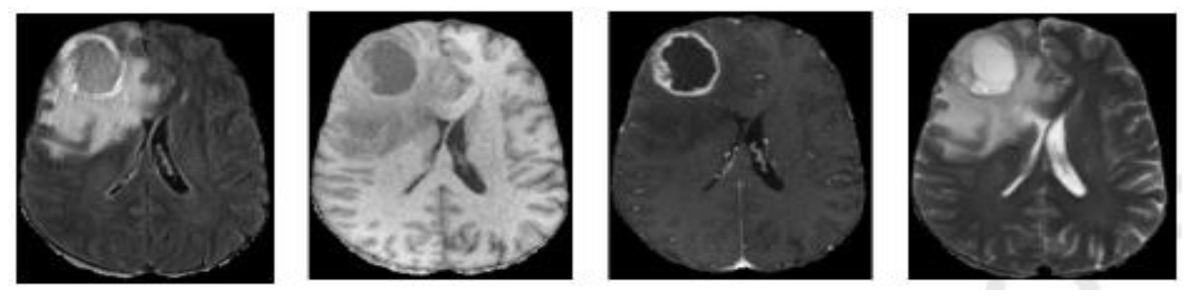
2.1.1. Dataset
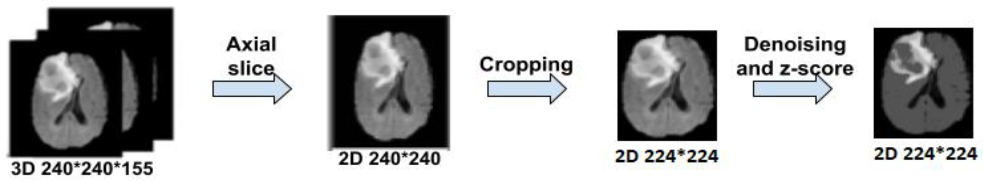
2.1.2. Data Preparation
2.2. Methods
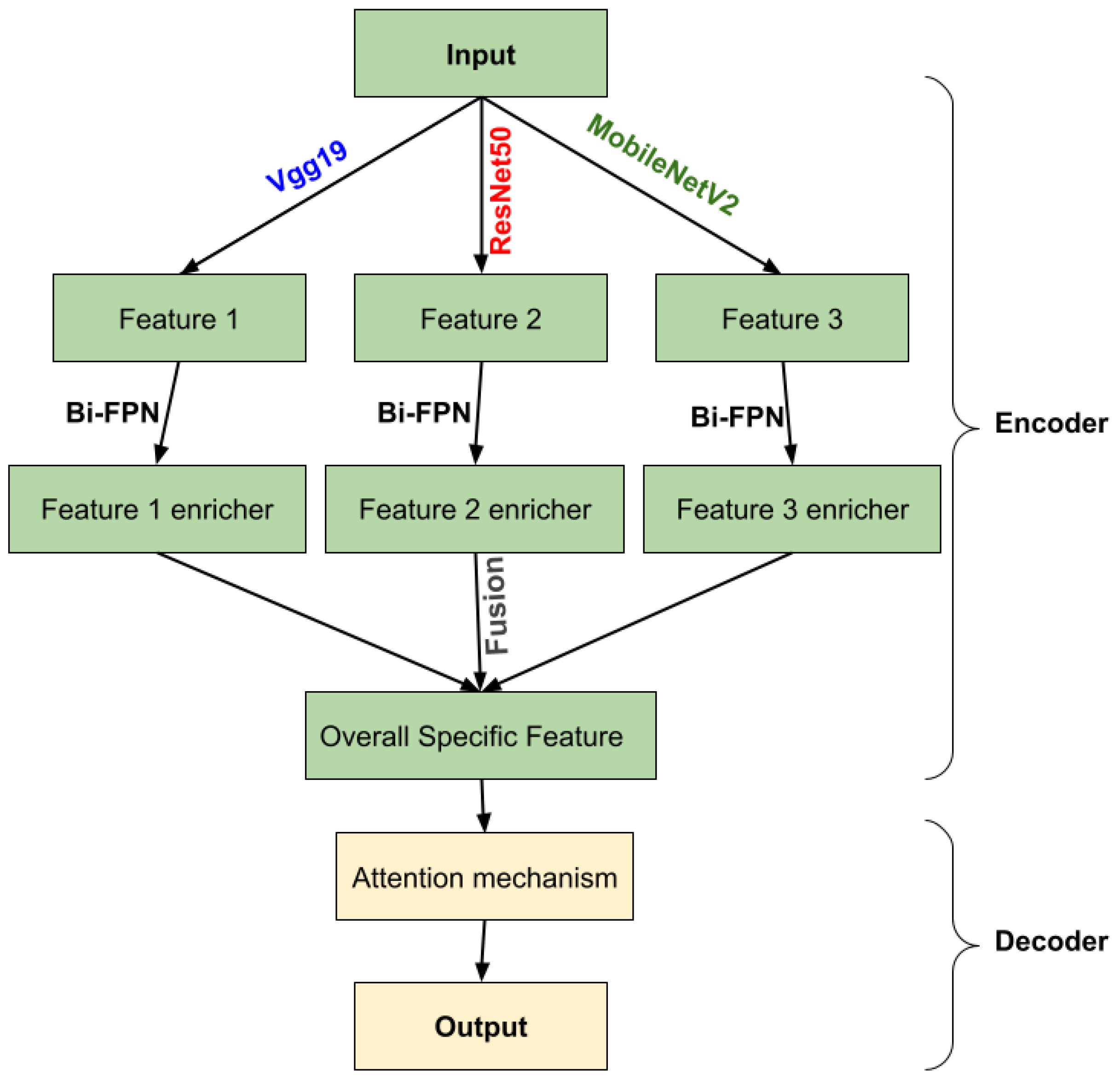
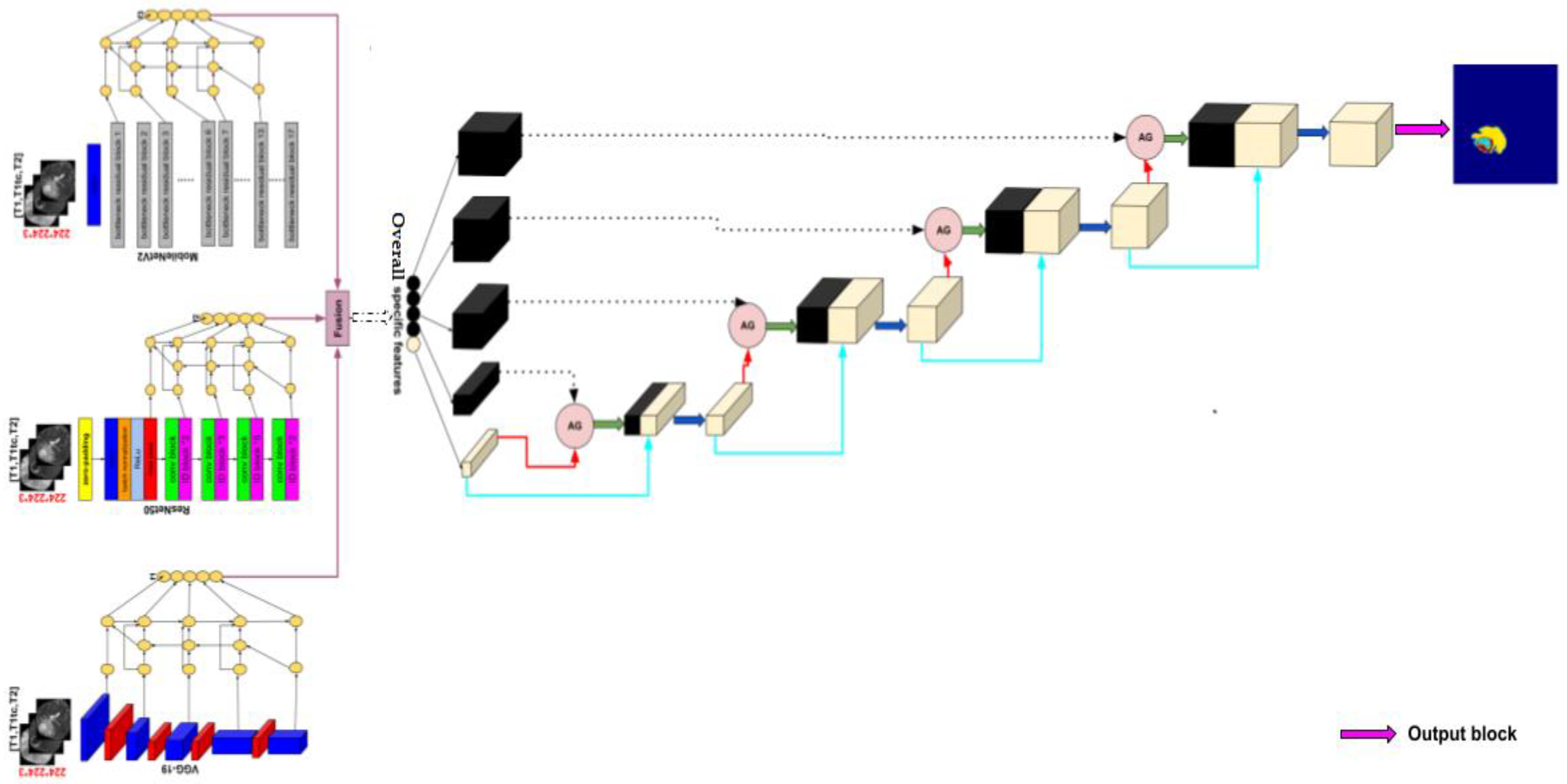
2.2.1. Encoder
Transfer Learning
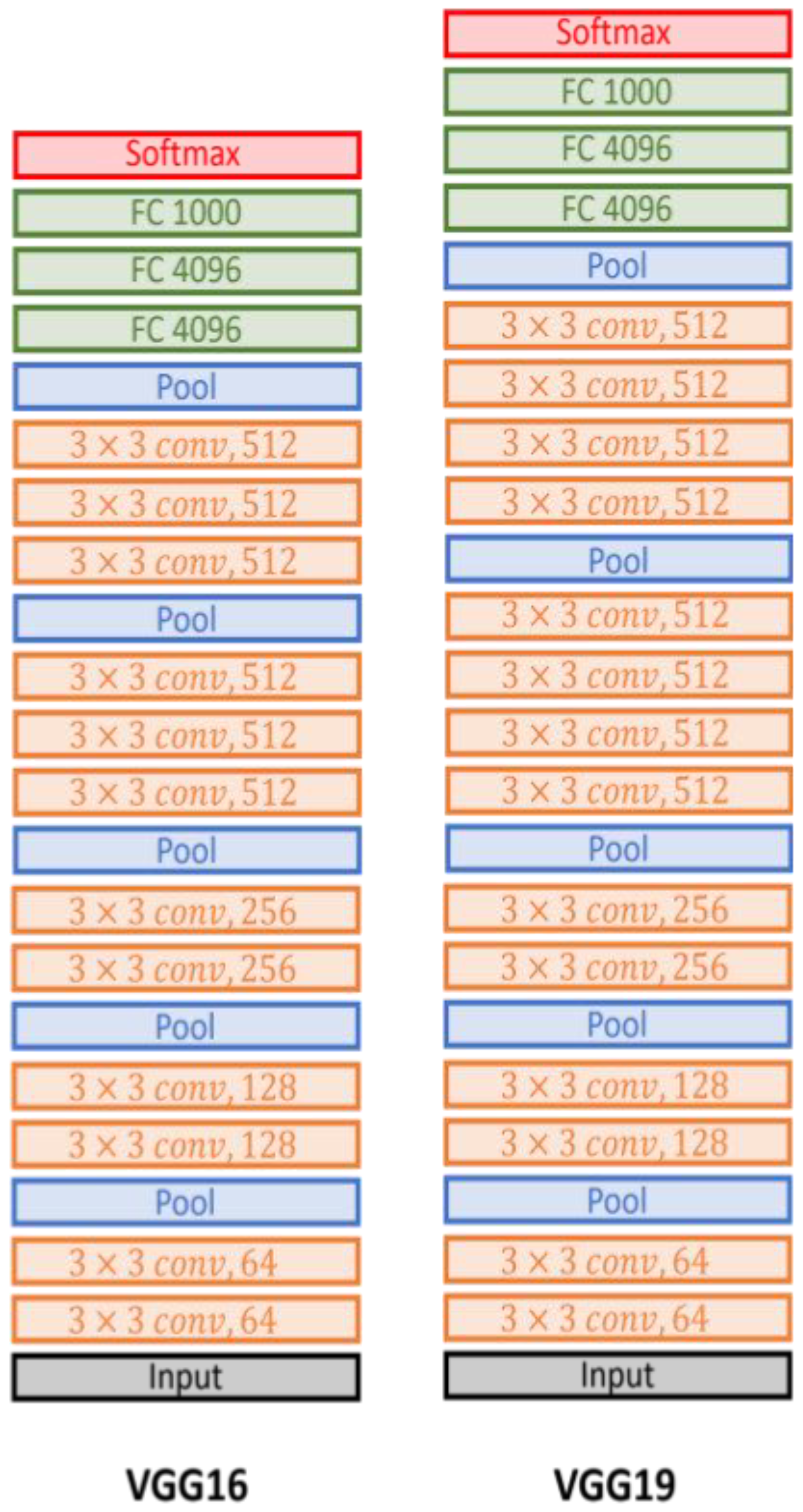
- VGG-19
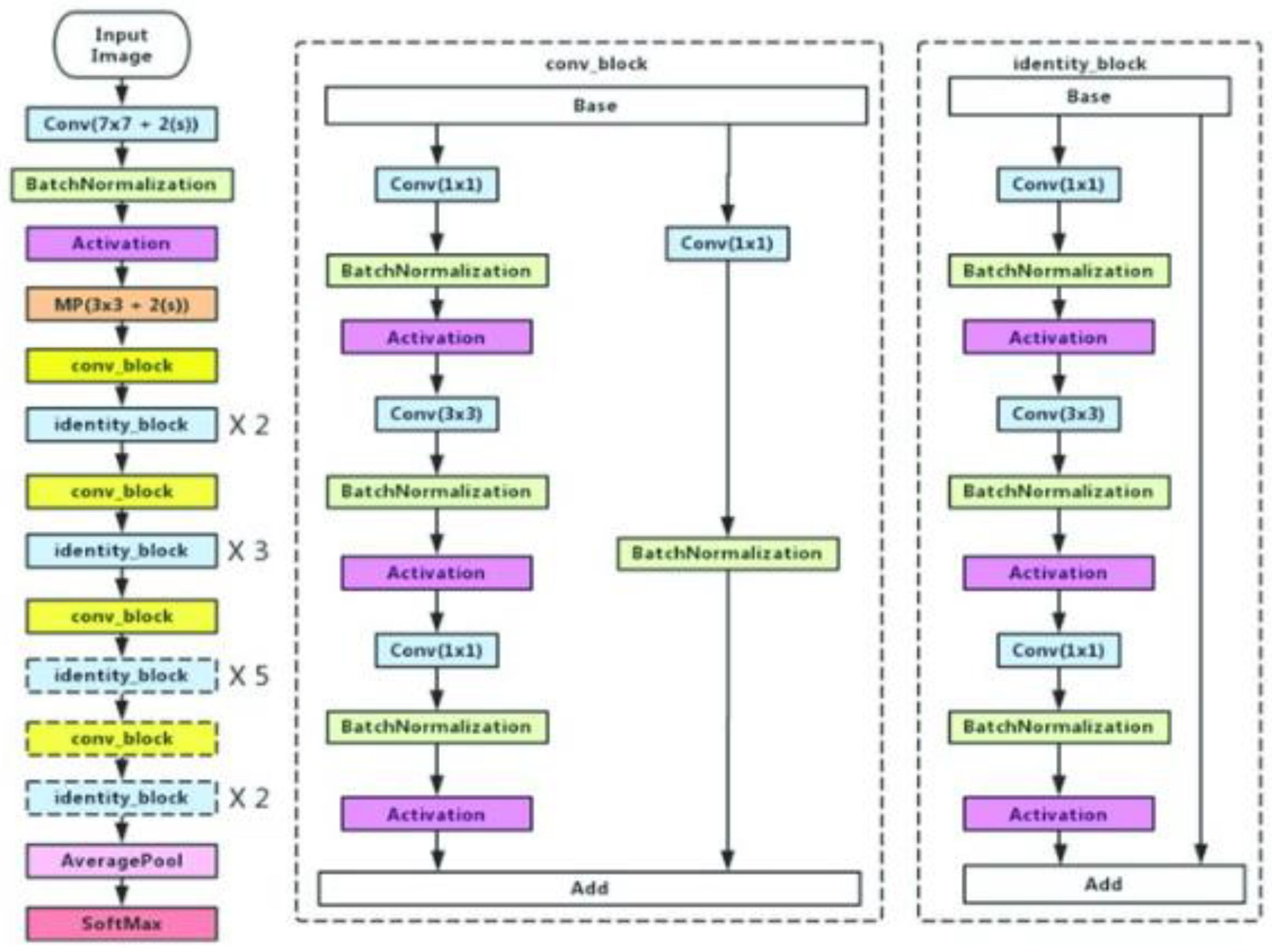
- ResNet50
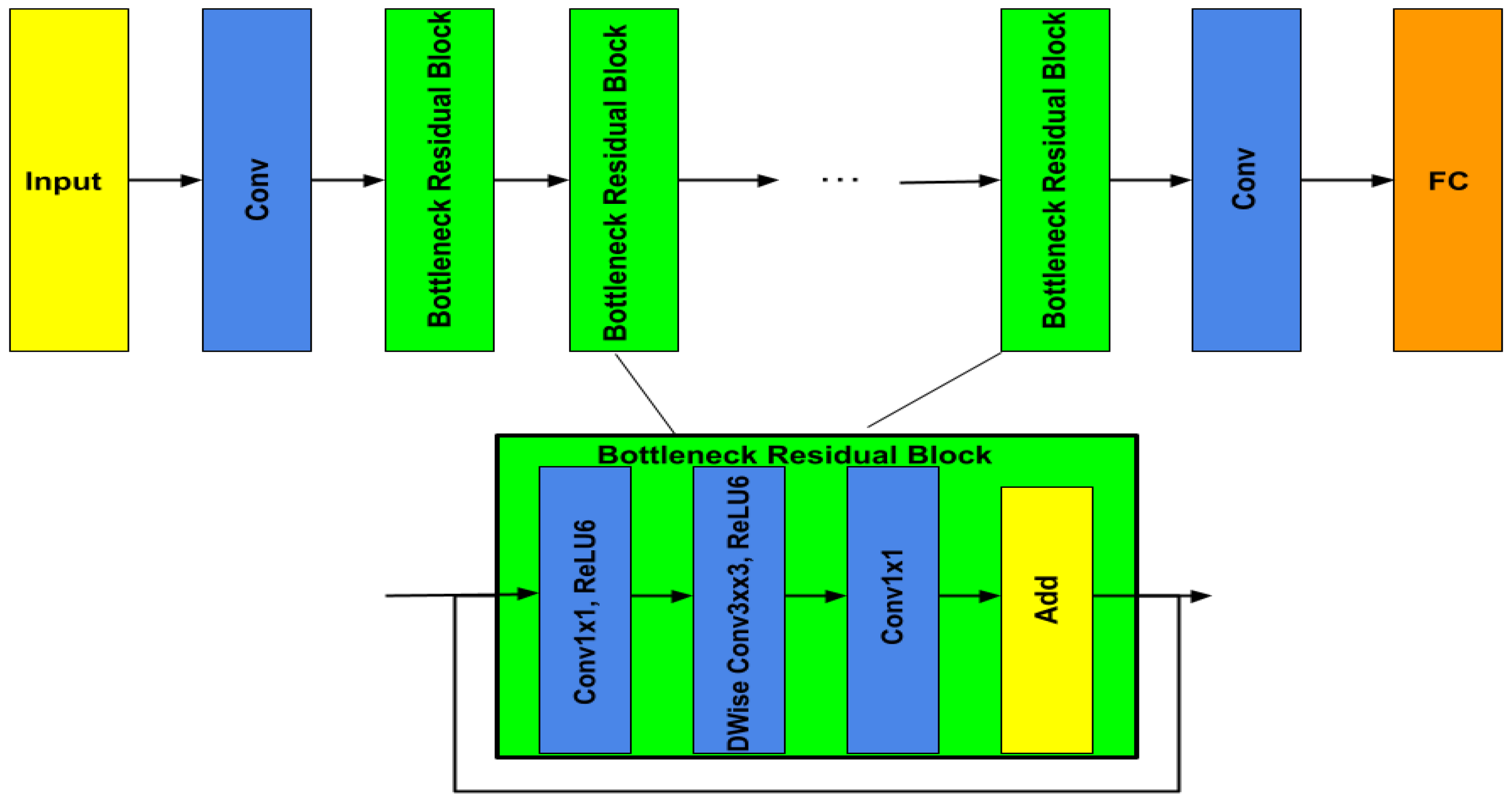
- MobileNetV2
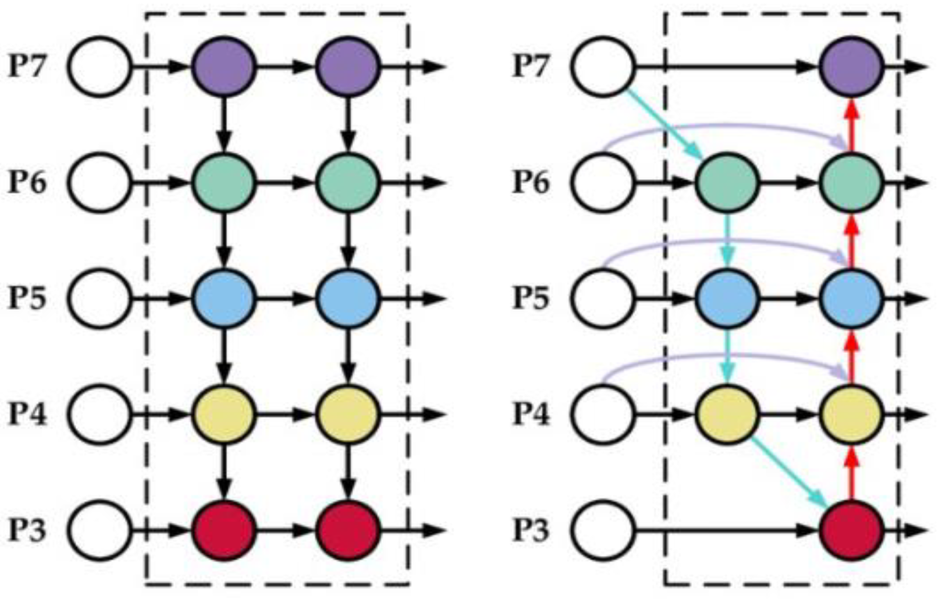
Bi-Directional Feature Pyramid Network (Bi-FPN)
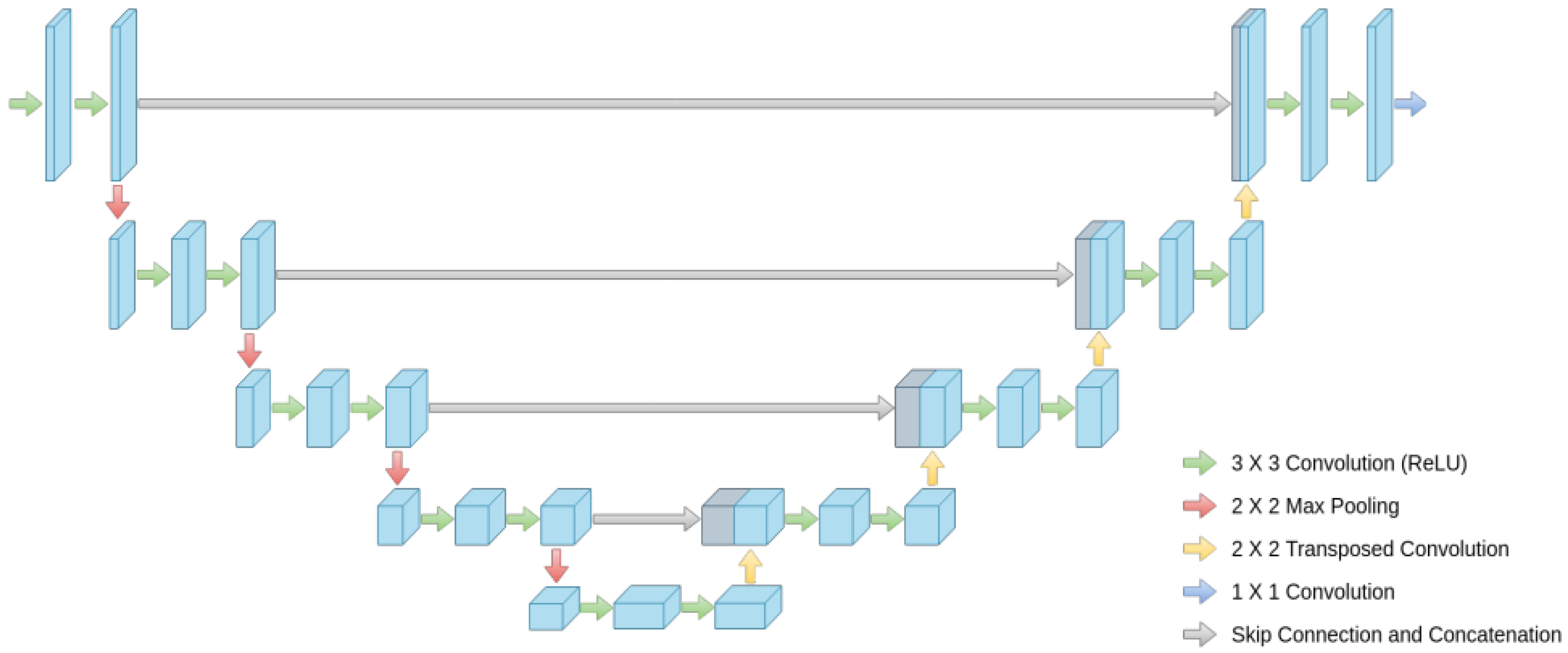
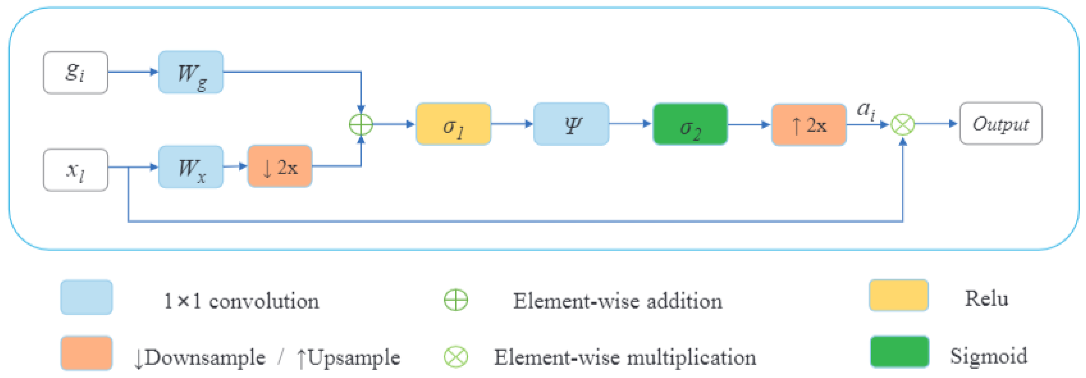
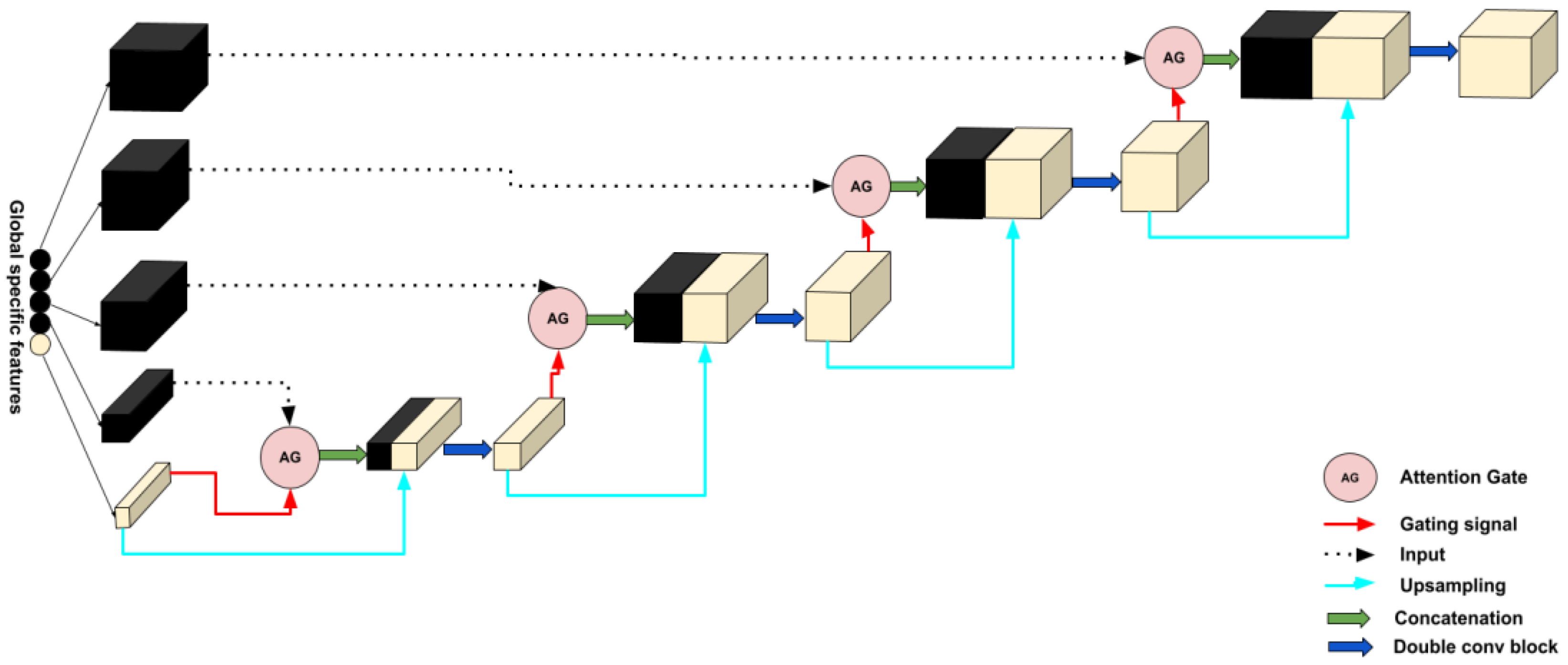
2.2.2. Decoder
3. Results
3.1. Implementation Details
3.2. Evaluation Metrics
- Accuracy: Formally, accuracy has the following definition:
- Precision: Formally, precision has the following definition:
- Recall: Formally, recall has the following definition:
- F1-score: Formally, F1-score has the following definition:
- The DSC represents the overlapping of predicted segmentation with the manually segmented output label and is computed as:
- The IoU is used when calculating mean average precision (mAP). It specifies the amount of overlap between the predicted and ground truth, and it is computed as:
- The Hausdorff95 distance measures the distance between the surface of the real area and the predicted area which is more sensitive to the segmented boundary defined as:
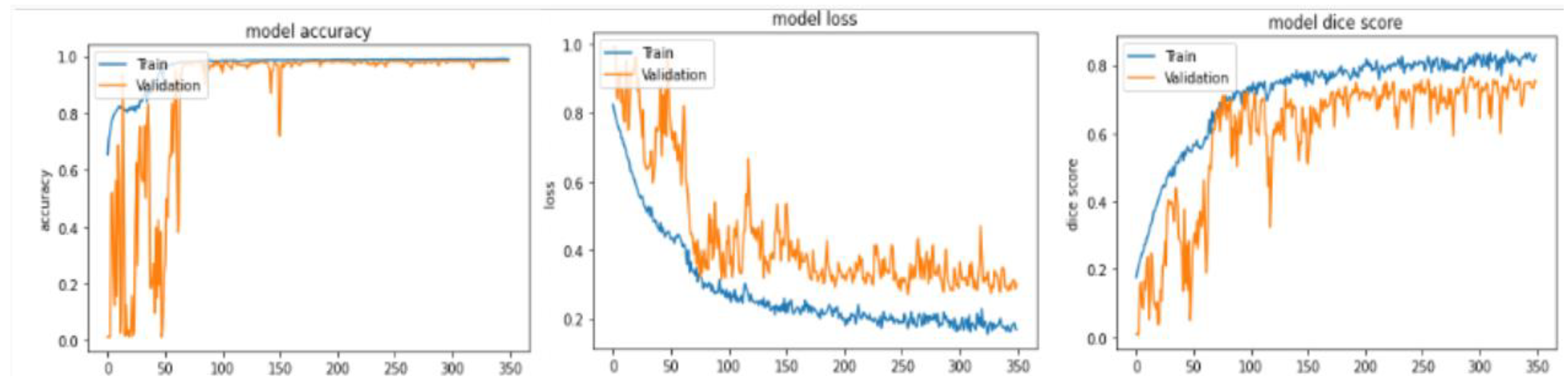
3.3. Results and Discussion
4. Conclusions
Author Contributions
Funding
Institutional Review Board Statement
Informed Consent Statement
Data Availability Statement
Conflicts of Interest
References
- Dhanachandra, N.; Manglem, K.; Chanu, Y.J. Image Segmentation Using K-means Clustering Algorithm and Subtractive Clustering Algorithm. Procedia Comput. Sci. 2015, 54, 764–771. [Google Scholar] [CrossRef]
- Kaur, N.; Sharma, M. Brain tumor detection using self-adaptive K-means clustering. In Proceedings of the 2017 International Conference on Energy, Communication, Data Analytics and Soft Computing (ICECDS), Chennai, India, 1–2 August 2017; pp. 1861–1865. [Google Scholar]
- Almahfud, M.A.; Setyawan, R.; Sari, C.A.; Rachmawanto, E.H. An effective MRI brain image segmentation using joint clustering (K-Means and Fuzzy C-Means). In Proceedings of the 2018 International Seminar on Research of Information Technology and Intelligent Systems (ISRITI), Yogyakarta, Indonesia, 21–22 November 2018; IEEE: New York, NY, USA, 2018. [Google Scholar]
- Chandra, G.R.; Rao, K.R.H. Tumor Detection In Brain Using Genetic Algorithm. Procedia Comput. Sci. 2016, 79, 449–457. [Google Scholar] [CrossRef]
- Cui, B.; Xie, M.; Wang, C. A Deep Convolutional Neural Network Learning Transfer to SVM-Based Segmentation Method for Brain Tumor. In Proceedings of the 2019 IEEE 11th International Conference on Advanced Infocomm Technology (ICAIT), Jinan, China, 18–20 October 2019; pp. 1–5. [Google Scholar]
- Chen, W.; Qiao, X.; Liu, B.; Qi, X.; Wang, R.; Wang, X. Automatic brain tumor segmentation based on features of separated local square. In Proceedings of the 2017 Chinese Automation Congress (CAC), Jinan, China, 20–22 October 2017. [Google Scholar]
- Hatami, T.; Hamghalam, M.; Reyhani-Galangashi, O.; Mirzakuchaki, S. A Machine Learning Approach to Brain Tumors Segmentation Using Adaptive Random Forest Algorithm. In Proceedings of the 2019 5th Conference on Knowledge Based Engineering and Innovation (KBEI), Tehran, Iran, 28 February–1 March 2019. [Google Scholar]
- Fulop, T.; Gyorfi, A.; Csaholczi, S.; Kovacs, L.; Szilagyi, L. Brain Tumor Segmentation from Multi-Spectral MRI Data Using Cascaded Ensemble Learning. In Proceedings of the 2020 IEEE 15th International Conference of System of Systems Engineering (SoSE), Budapest, Hungary, 2–4 June 2020. [Google Scholar]
- Shen, D.; Wu, G.; Suk, H.-I. Deep Learning in Medical Image Analysis. Annu. Rev. Biomed. Eng. 2017, 19, 221–248. [Google Scholar] [CrossRef] [PubMed]
- Qayyum, A.; Anwar, S.M.; Awais, M.; Majid, M. Medical image retrieval using deep convolutional neural network. arXiv 2017, arXiv:1703.08472. [Google Scholar] [CrossRef]
- Pereira, S.; Pinto, A.; Alves, V.; Silva, C.A. Brain Tumor Segmentation Using Convolutional Neural Networks in MRI Images. IEEE Trans. Med. Imaging 2016, 35, 1240–1251. [Google Scholar] [CrossRef] [PubMed]
- Zhao, X.; Wu, Y.; Song, G.; Li, Z.; Fan, Y.; Zhang, Y. Brain tumor segmentation using a fully convolutional neural network withconditional random fields. In International Workshop on Brainlesion: Glioma, Multiple Sclerosis, Stroke and Traumatic Brain Injuries; Springer: Cham, Switzerland, 2016; pp. 75–87. [Google Scholar]
- Wang, G.; Li, W.; Ourselin, S.; Vercauteren, T. Automatic brain tumor segmentation using cascaded anisotropic convolution-alneural networks. In International MICCAI Brainlesion Workshop; Springer: Cham, Switzerland, 2017; pp. 178–190. [Google Scholar]
- Aboussaleh, I.; Riffi, J.; Mahraz, A.M.; Tairi, H. Brain Tumor Segmentation Based on Deep Learning’s Feature Representation. J. Imaging 2021, 7, 269. [Google Scholar] [CrossRef] [PubMed]
- Ronneberger, O.; Fischer, P.; Brox, T. U-net: Convolutional networks for biomedical image segmentation. In Proceedings of the 18th International Conference on Medical Image Computing and Computer-Assisted Intervention–MICCAI 2015, Munich, Germany, 5–9 October 2015; Springer: Cham, Switzerland, 2015. [Google Scholar]
- Liu, H.; Shen, X.; Shang, F.; Ge, F.; Wang, F. CU-Net: Cascaded U-Net with loss weighted sampling for brain tumor segmentation. In Multimodal Brain Image Analysis and Mathematical Foundations of Computational Anatomy; Springer: Cham, Switzerland, 2019; pp. 102–111. [Google Scholar]
- Aboelenein, N.M.; Songhao, P.; Koubaa, A.; Noor, A.; Afifi, A. HTTU-Net: Hybrid Two Track U-Net for Automatic Brain Tumor Segmentation. IEEE Access 2020, 8, 101406–101415. [Google Scholar] [CrossRef]
- Pravitasari, A.A.; Iriawan, N.; Almuhayar, M.; Azmi, T.; Irhamah, I.; Fithriasari, K.; Purnami, S.W.; Ferriastuti, W. UNet-VGG16 with transfer learning for MRI-based brain tumor segmentation. TELKOMNIKA (Telecommun. Comput. Electron. Control.) 2020, 18, 1310–1318. [Google Scholar] [CrossRef]
- Kamilaris, A.; Prenafeta-Boldú, F.X. A review of the use of convolutional neural networks in agriculture. J. Agric. Sci. 2018, 156, 312–322. [Google Scholar] [CrossRef]
- Lecun, Y.; Bottou, L.; Bengio, Y.; Haffner, P. Gradient-based learning applied to document recognition. Proc. IEEE 1998, 86, 2278–2324. [Google Scholar] [CrossRef]
- Krizhevsky, A.; Sutskever, I.; Hinton, G.E. Imagenet Classification with Deep Convolutional Neural Networks. In Advances in Neural Information Processing Systems; 2012; pp. 1097–1105. Available online: https://proceedings.neurips.cc/paper/4824-imagenet-classification-with-deep-convolutional-neural-networks.pdf (accessed on 20 February 2023).
- Howard, A.G.; Zhu, M.; Chen, B.; Kalenichenko, D.; Wang, W.; Weyand, T.; Andreetto, M.; Adam, H. Mobilenets: Efficient convolutional neural networks for mobile vision applications. arXiv 2017, arXiv:1704.04861. [Google Scholar]
- Xie, S.; Girshick, R.; Dollár, P.; Tu, Z.; He, K. Aggregated residual transformations for deep neural networks. In Proceedings of the IEEE Conference on Computer Vision and Pattern Recognition, Honolulu, HI, USA, 21–26 July 2017. [Google Scholar]
- Zhang, J.; Jiang, Z.; Dong, J.; Hou, Y.; Liu, B. Attention gate resU-Net for automatic MRI brain tumor segmentation. IEEE Access 2020, 8, 58533–58545. [Google Scholar] [CrossRef]
- Wu, X.; Bi, L.; Fulham, M.; Feng, D.D.; Zhou, L.; Kim, J. Unsupervised brain tumor segmentation using a symmetric-driven adversarial network. Neurocomputing 2021, 455, 242–254. [Google Scholar] [CrossRef]
- Dey, R.; Hong, Y. Asc-net: Adversarial-based selective network for unsupervised anomaly segmentation. In Proceedings of the 24th International Conference on Medical Image Computing and Computer Assisted Intervention—MICCAI 2021, Strasbourg, France, 27 September–1 October 2021; Springer: Cham, Switzerland, 2021. [Google Scholar]
- Menze, B.H.; Jakab, A.; Bauer, S.; Kalpathy-Cramer, J.; Farahani, K.; Kirby, J.; Burren, Y.; Porz, N.; Slotboom, J.; Wiest, R.; et al. The Multimodal Brain Tumor Image Segmentation Benchmark (BRATS). IEEE Trans. Med. Imaging 2015, 34, 1993–2024. [Google Scholar] [CrossRef] [PubMed]
- Bakas, S.; Akbari, H.; Sotiras, A.; Bilello, M.; Rozycki, M.; Kirby, J.S.; Freymann, J.B.; Farahani, K.; Davatzikos, C. Advancing The Cancer Genome Atlas glioma MRI collections with expert segmentation labels and radiomic features. Sci. Data 2017, 4, 170117. [Google Scholar] [CrossRef] [PubMed]
- Bakas, S.; Reyes, M.; Jakab, A.; Bauer, S.; Rempfler, M.; Crimi, A.; Shinohara, R.T.; Berger, C.; Ha, S.M.; Rozycki, M.; et al. Identifying the Best Machine Learning Algorithms for Brain Tumor Segmentation, Progression Assessment, and Overall Survival Prediction in the BRATS Challenge. arXiv 2018, arXiv:1811.02629. [Google Scholar]
- Zoph, B.; Vasudevan, V.; Shlens, J.; Le, Q.V. Learning transferable architectures for scalable image recognition. In Proceedings of the IEEE Conference on Computer Vision and Pattern Recognition, Salt Lake City, UT, USA, 18–23 June 2018. [Google Scholar]
- Lin, T.Y.; Dollár, P.; Girshick, R.; He, K.; Hariharan, B.; Belongie, S. Feature pyramid networks for object detection. In Proceedings of the IEEE Conference on Computer Vision and Pattern Recognition, Honolulu, HI, USA, 21–26 July 2017. [Google Scholar]
- Kong, T.; Sun, F.; Tan, C.; Liu, H.; Huang, W. Deep feature pyramid reconfiguration for object detection. In Proceedings of the Computer Vision—ECCV 2018: 15th European Conference, Munich, Germany, 8–14 September 2018. [Google Scholar]
- Kim, S.-W.; Kook, H.-K.; Sun, J.-Y.; Kang, M.-C.; Ko, S.-J. Parallel feature pyramid network for object detection. In Proceedings of the Computer Vision–ECCV 2018: 15th European Conference, Munich, Germany, 8–14 September 2018. [Google Scholar]
- Zhao, Q.; Sheng, T.; Wang, Y.; Tang, Z.; Chen, Y.; Cai, L.; Ling, H. M2Det: A Single-Shot Object Detector Based on Multi-Level Feature Pyramid Network. In Proceedings of the AAAI Conference on Artificial Intelligence, Honolulu, HI, USA, 27 January–1 February 2019; AAAI: Menlo Park, CA, USA, 2019. [Google Scholar]
- Chollet, F. Xception: Deep learning with depthwise separable convolutions. In Proceedings of the 2017 IEEE Conference on Computer Vision and Pattern Recognition (CVPR), Honolulu, HI, USA, 21–26 July 2017; pp. 1610–02357. [Google Scholar]
- Shen, T.; Zhou, T.; Long, G.; Jiang, J.; Pan, S.; Zhang, C. Disan: Directional self-attention network for RNN/CNN-free language understanding. In Proceedings of the 32th AAAI Conference on Artificial Intelligence, New Orleans, LA, USA, 2–7 February 2018; pp. 5446–5455. [Google Scholar]
- Kronberg, R.M.; Meskelevicius, D.; Sabel, M.; Kollmann, M.; Rubbert, C.; Fischer, I. Optimal acquisition sequence for AI-assisted brain tumor segmentation under the constraint of largest information gain per additional MRI sequence. Neurosci. Inform. 2022, 2, 100053. [Google Scholar] [CrossRef]
- Sudre, C.H.; Li, W.; Vercauteren, T.; Ourselin, S.; Jorge Cardoso, M. Generalised dice overlap as a deep learning loss function for highly unbalanced segmentations. In Deep Learning in Medical Image Analysis and Multimodal Learning for Clinical Decision Support; Springer: Cham, Switzerland, 2017; pp. 240–248. [Google Scholar]
- Mahmud, M.R.; Mamun, M.A.; Hossain, M.A.; Uddin, M.P. Comparative Analysis of K-Means and Bisecting K-Means Algo-rithms for Brain Tumor Detection. In Proceedings of the 2018 International Conference on Computer, Communication, Chemical, Material and Electronic Engineering (IC4ME2), Rajshahi, Bangladesh, 8–9 February 2018. [Google Scholar]
- He, H.; Fang, L. Three pathways U-Net for brain tumor segmentation. In Pre-Conference Proceedings of the 7th Medical Image Computing and Computer-Assisted Interventions (MICCAI) BraTS Challenge, Granada, Spain, 16 September 2018; pp. 119–126. [Google Scholar]
- Chen, W.; Liu, B.; Peng, S.; Sun, J.; Qiao, X. S3D-UNET: Separable 3D U-Net for brain tumor segmentation. In Proceedings of the 4th International Workshop, Brainlesion: Glioma, Multiple Sclerosis, Stroke and Traumatic Brain Injuries, BrainLes 2018, Held in Conjunction with MICCAI 2018, Granada, Spain, 16 September 2018; Lecture Notes in Computer Science. Springer: Berlin, Germany, 2019; Volume 11384. [Google Scholar]
- Chen, S.; Ding, C.; Liu, M. Dual-force convolutional neural networks for accurate brain tumor segmentation. Pattern Recognit. 2019, 88, 90–100. [Google Scholar] [CrossRef]


| Layer | Output Size |
|---|---|
| Input | (224,224,3) |
| VGG-19 + BiFPN 1 | [(224,224,32), (112,112,32), (56,56,32), (28,28,32), (14,14,32)] |
| MobileNetV2 + BiFPN 2 | [(224,224,32), (112,112,32), (56,56,32), (28,28,32), (14,14,32)] |
| ResNet50 + BiFPN 3 | [(224,224,32), (112,112,32), (56,56,32), (28,28,32), (14,14,32)] |
| Fusion of 1, 2, and 3 | [(224,224,32), (112,112,32), (56,56,32), (28,28,32), (14,14,32)] |
| Attention decoder | (224,224,128) |
| Output | (224,224,4) |
| Subset | DSC (%) | IoU (%) | HD95(mm) | ||||||
|---|---|---|---|---|---|---|---|---|---|
| WT | TC | EnT | WT | TC | EnT | WT | TC | EnT | |
| Training | 92.11 | 90.30 | 88.78 | 82.25 | 78.90 | 76.55 | 0.0 | 1.00 | 0 |
| Validation | 87.89 | 76.45 | 67.63 | 78.39 | 61.88 | 51.09 | 0.0 | 2.00 | 2.84 |
| Test | 87.41 | 80.69 | 70.33 | 77.64 | 67.63 | 54.24 | 0.0 | 1.00 | 0.0 |
| Subset | Precision (%) | F1-Score (%) | Recall (%) | Accuracy (%) | ||||||||
|---|---|---|---|---|---|---|---|---|---|---|---|---|
| WT | TC | EnT | WT | TC | EnT | WT | TC | EnT | WT | TC | EnT | |
| Training | 91.19 | 90.65 | 88.41 | 90.5 | 89.13 | 86.19 | 90.08 | 88.77 | 84.06 | 99.90 | 99.45 | 98.79 |
| Validation | 87.50 | 85.34 | 83.66 | 87.3 | 84.91 | 82.44 | 86.22 | 84.04 | 82.15 | 99.20 | 98.10 | 97.15 |
| Test | 90.40 | 89.79 | 86.23 | 88.9 | 88.54 | 83.93 | 87.88 | 87.04 | 82.98 | 99.77 | 99.23 | 98.30 |
| Method | Data | Performance of (%) | ||
|---|---|---|---|---|
| WT | TC | EnT | ||
| Bisecting (no initialization) [39] | MRI collected by authors | ACC 83.05 | - | - |
| Aboussaleh et al. [14] | BraTS2017 | DSC 82.35 | - | - |
| Wu et al. [25] | BraTS2018 | DSC (avg) 61.90 | - | - |
| K-means and FCM [3] | https://radiopaedia.org/ (accessed on 1 September 2022) | ACC 56.40 | - | - |
| U-Net [15] | BraTS2020 | DSC 80 | DSC 62 | DSC 60 |
| U-Net-VGG16 [18] | Data approved by Dr. Soetomo Surabaya | ACC (avg) 96.10 | - | - |
| Single path MLDeepMedic [42] | BraTS2017 | DSC 79.73 | DSC 71.59 | DSC 68.14 |
| Fang et al. [40] | BraTS2018 | DSC 85.60 | DSC 72.20 | DSC 72.60 |
| Chen et al. [41] | BraTS2018 | DSC 83.60 | DSC 68.90 | DSC 78.30 |
| HTTU-Net [17] | BraTS2018 | DSC 86.50 | DSC 74.50 | DSC 80.80 |
| AGResU-Net [24] | BraTS2019 | DSC 87 | DSC 77.70 | DSC 70.90 |
| Our method | BraTS2020 | DSC 87.41 | DSC 80.69 | DSC 70.33 |
| Method | DSC (%) | IoU (%) | HD96 (mm) | Accuracy (%) | ||||||
|---|---|---|---|---|---|---|---|---|---|---|
| WT | TC | EnT | WT | TC | EnT | WT | TC | EnT | AVG | |
| U-Net | 80.0 | 62.0 | 60.0 | 67.0 | 52.0 | 42.0 | 2.84 | 2.0 | 2.83 | 92.0 |
| VGG-19 + Decoder | 81.32 | 75.13 | 61.66 | 68.53 | 60.17 | 44.57 | 2.0 | 2.00 | 0.0 | 97.26 |
| MobileNetV2 + Decoder | 86.43 | 80.51 | 71.25 | 76.11 | 67.44 | 55.34 | 1.0 | 1.00 | 0.0 | 97.0 |
| ResNet50 + Decoder | 85.78 | 78.77 | 70.51 | 75.09 | 64.97 | 54.45 | 2.0 | 1.13 | 0.0 | 97.0 |
| 3Encoder + Decoder | 84.77 | 77.13 | 67.01 | 73.57 | 62.77 | 50.39 | 2.0 | 1.41 | 0.0 | 98.29 |
| 3Encoder + AttDecoder | 79.16 | 72.89 | 61.92 | 62.86 | 55.86 | 45.07 | 3.0 | 2.00 | 0.0 | 97.11 |
| 3Encoder + BiFPN + Decoder | 86.88 | 80.55 | 70.11 | 76.58 | 67.51 | 54.11 | 0.0 | 1.00 | 0.0 | 98.99 |
| 3Encoder + BiFPN+ AttDecoder (our method) | 87.41 | 80.69 | 70.33 | 77.64 | 67.63 | 54.24 | 0.0 | 1.0 | 0.0 | 99.10 |
Disclaimer/Publisher’s Note: The statements, opinions and data contained in all publications are solely those of the individual author(s) and contributor(s) and not of MDPI and/or the editor(s). MDPI and/or the editor(s) disclaim responsibility for any injury to people or property resulting from any ideas, methods, instructions or products referred to in the content. |
© 2023 by the authors. Licensee MDPI, Basel, Switzerland. This article is an open access article distributed under the terms and conditions of the Creative Commons Attribution (CC BY) license (https://creativecommons.org/licenses/by/4.0/).
Share and Cite
Aboussaleh, I.; Riffi, J.; Fazazy, K.E.; Mahraz, M.A.; Tairi, H. Efficient U-Net Architecture with Multiple Encoders and Attention Mechanism Decoders for Brain Tumor Segmentation. Diagnostics 2023, 13, 872. https://doi.org/10.3390/diagnostics13050872
Aboussaleh I, Riffi J, Fazazy KE, Mahraz MA, Tairi H. Efficient U-Net Architecture with Multiple Encoders and Attention Mechanism Decoders for Brain Tumor Segmentation. Diagnostics. 2023; 13(5):872. https://doi.org/10.3390/diagnostics13050872
Chicago/Turabian StyleAboussaleh, Ilyasse, Jamal Riffi, Khalid El Fazazy, Mohamed Adnane Mahraz, and Hamid Tairi. 2023. "Efficient U-Net Architecture with Multiple Encoders and Attention Mechanism Decoders for Brain Tumor Segmentation" Diagnostics 13, no. 5: 872. https://doi.org/10.3390/diagnostics13050872
APA StyleAboussaleh, I., Riffi, J., Fazazy, K. E., Mahraz, M. A., & Tairi, H. (2023). Efficient U-Net Architecture with Multiple Encoders and Attention Mechanism Decoders for Brain Tumor Segmentation. Diagnostics, 13(5), 872. https://doi.org/10.3390/diagnostics13050872