
Deep Features from Pretrained Networks Do Not Outperform Hand-Crafted Features in Radiomics


Abstract
:1. Introduction
2. Related Works
3. Materials and Methods
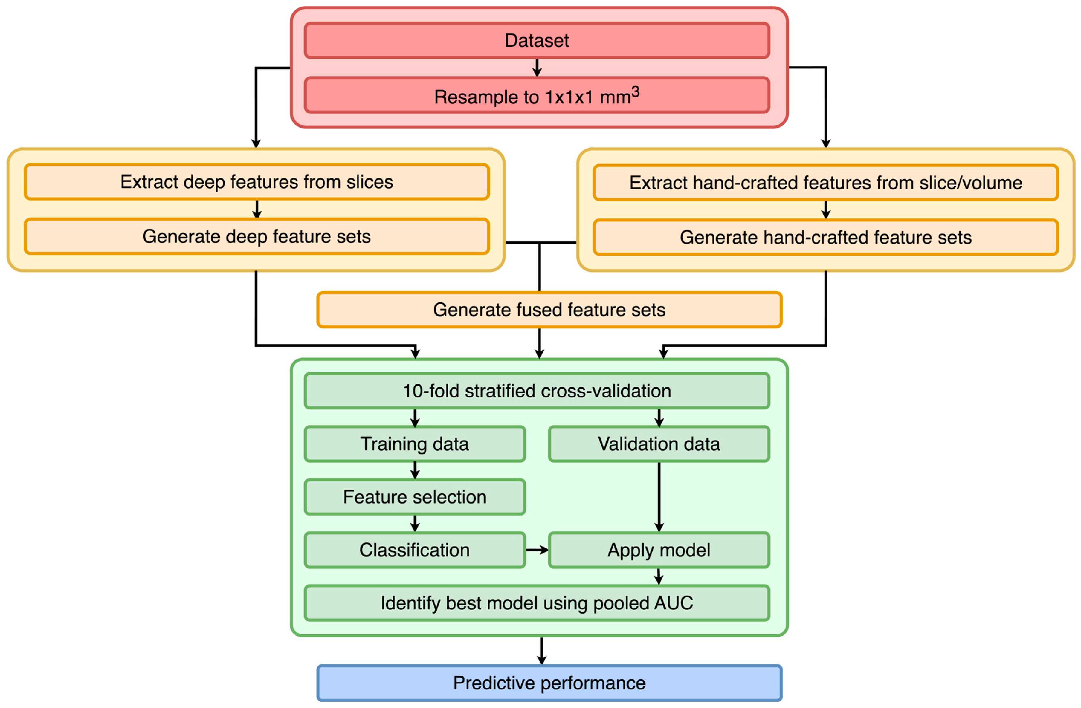
3.1. Study Design
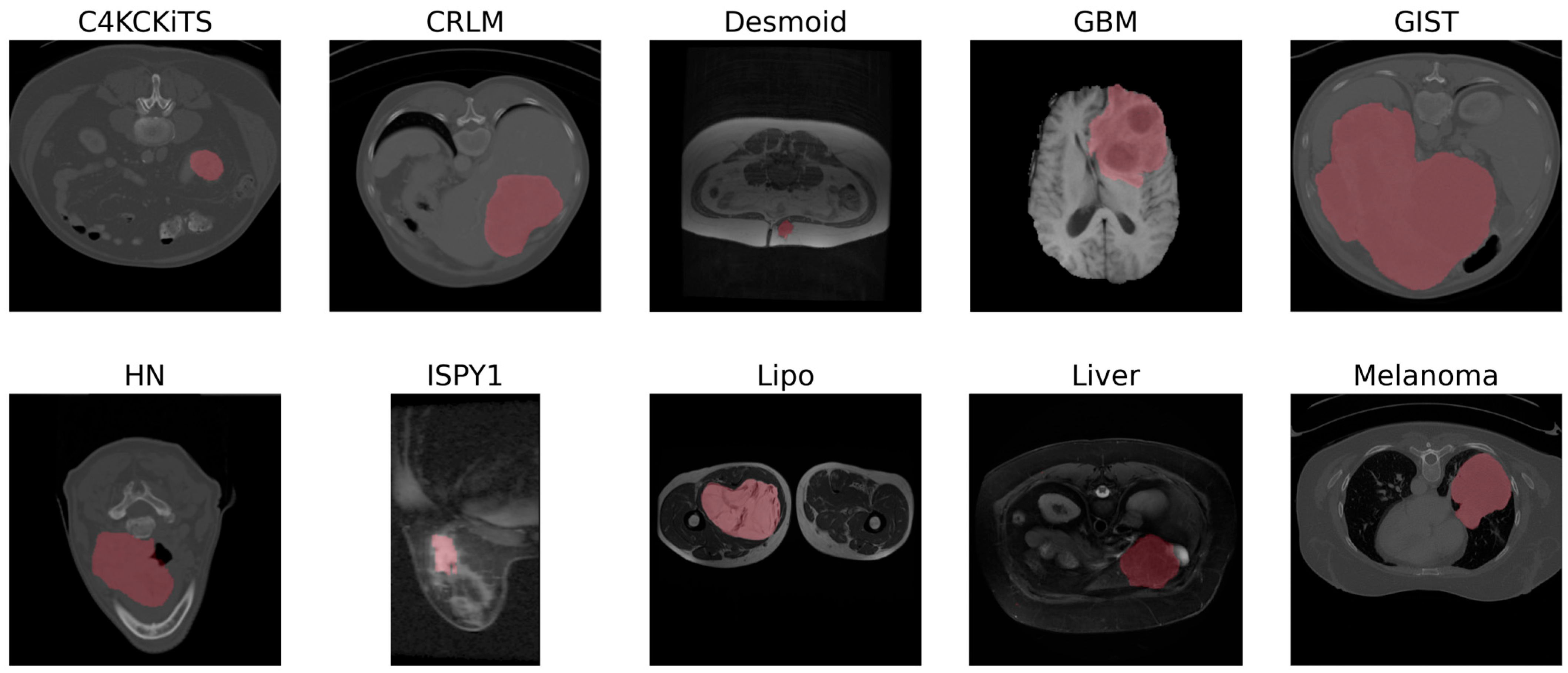
3.2. Datasets
3.3. Preprocessing
3.4. Feature Extraction
3.5. Training
3.6. Performance Metrics
3.7. Evaluation
3.8. Experimental Settings
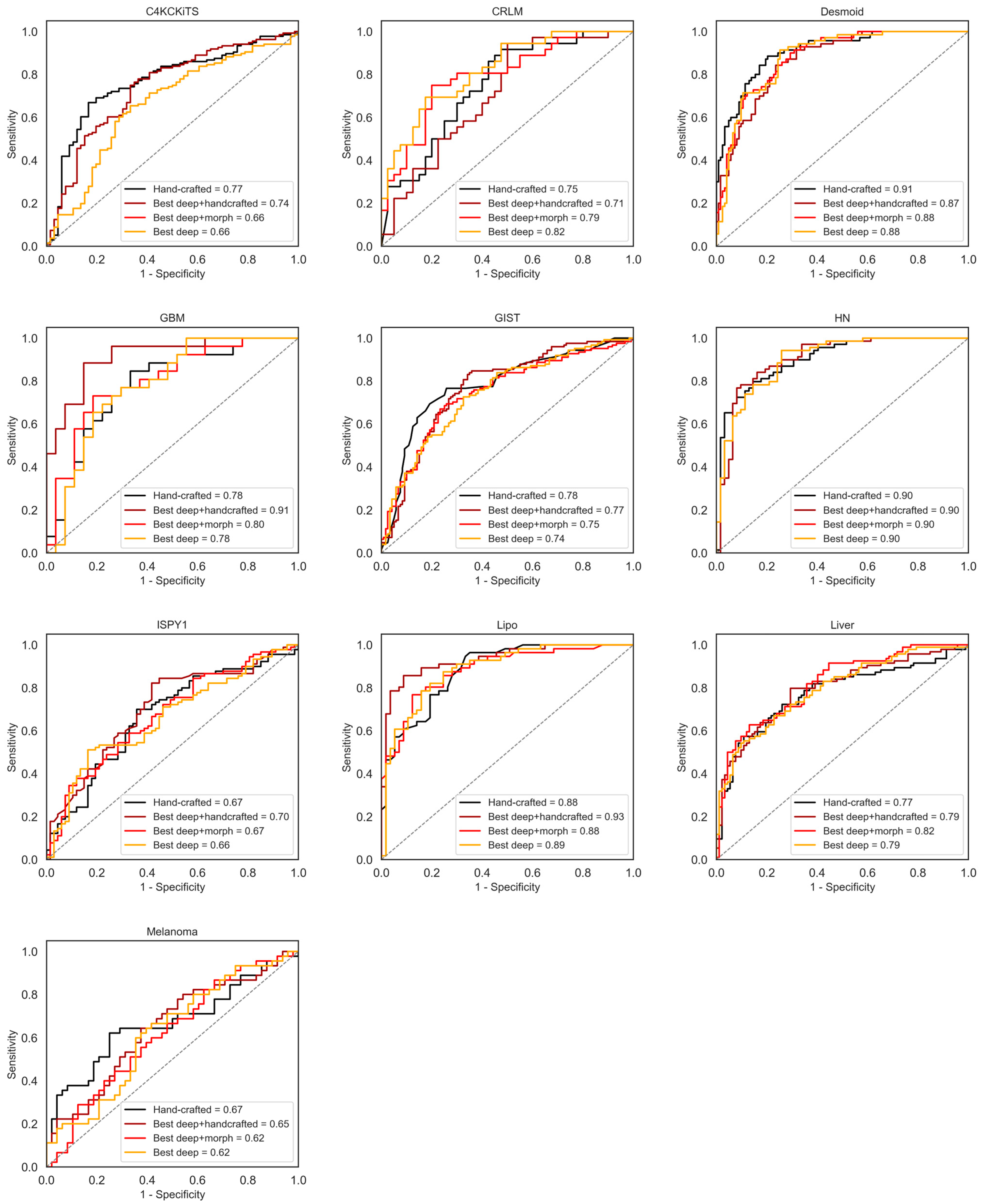
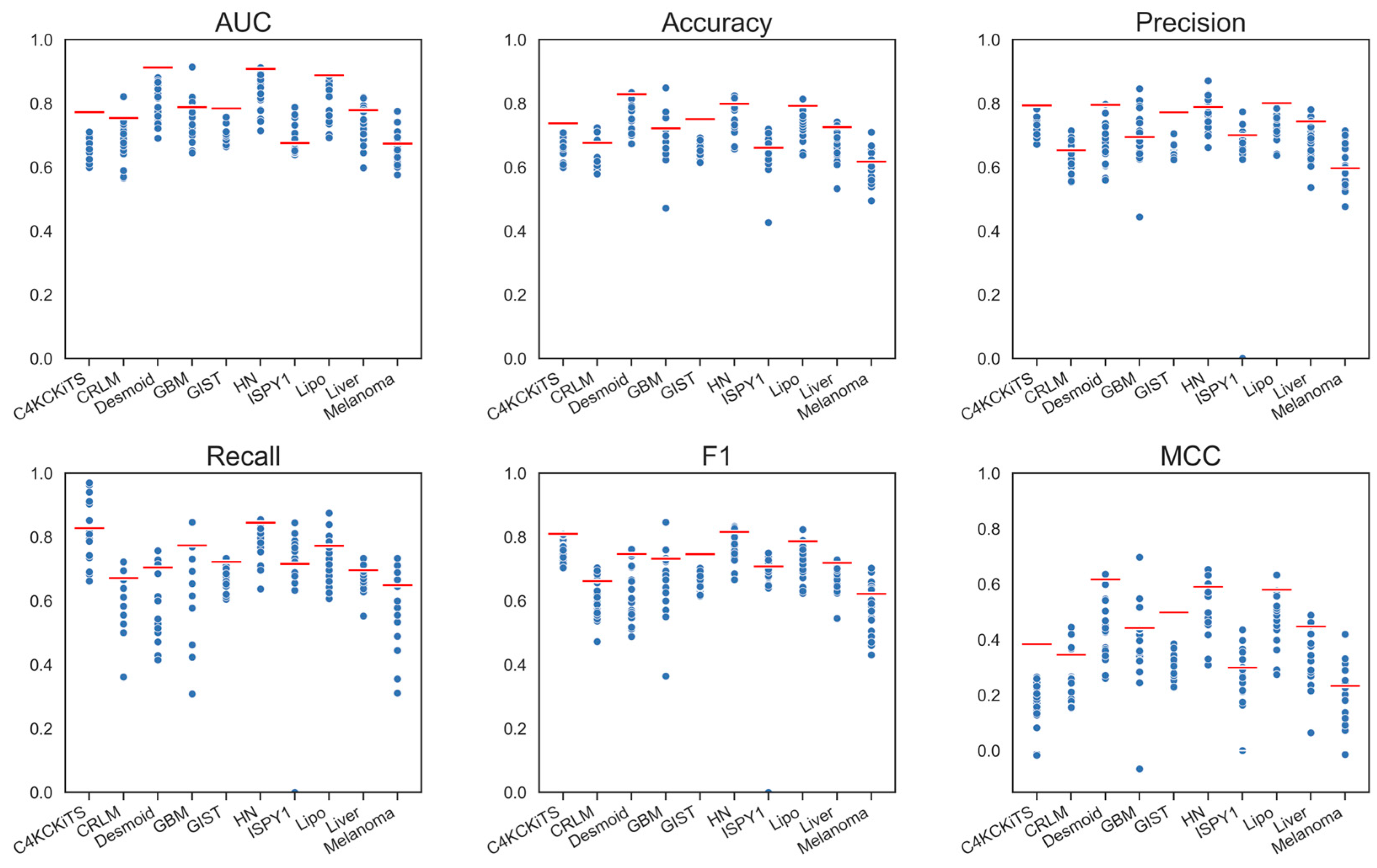
4. Results
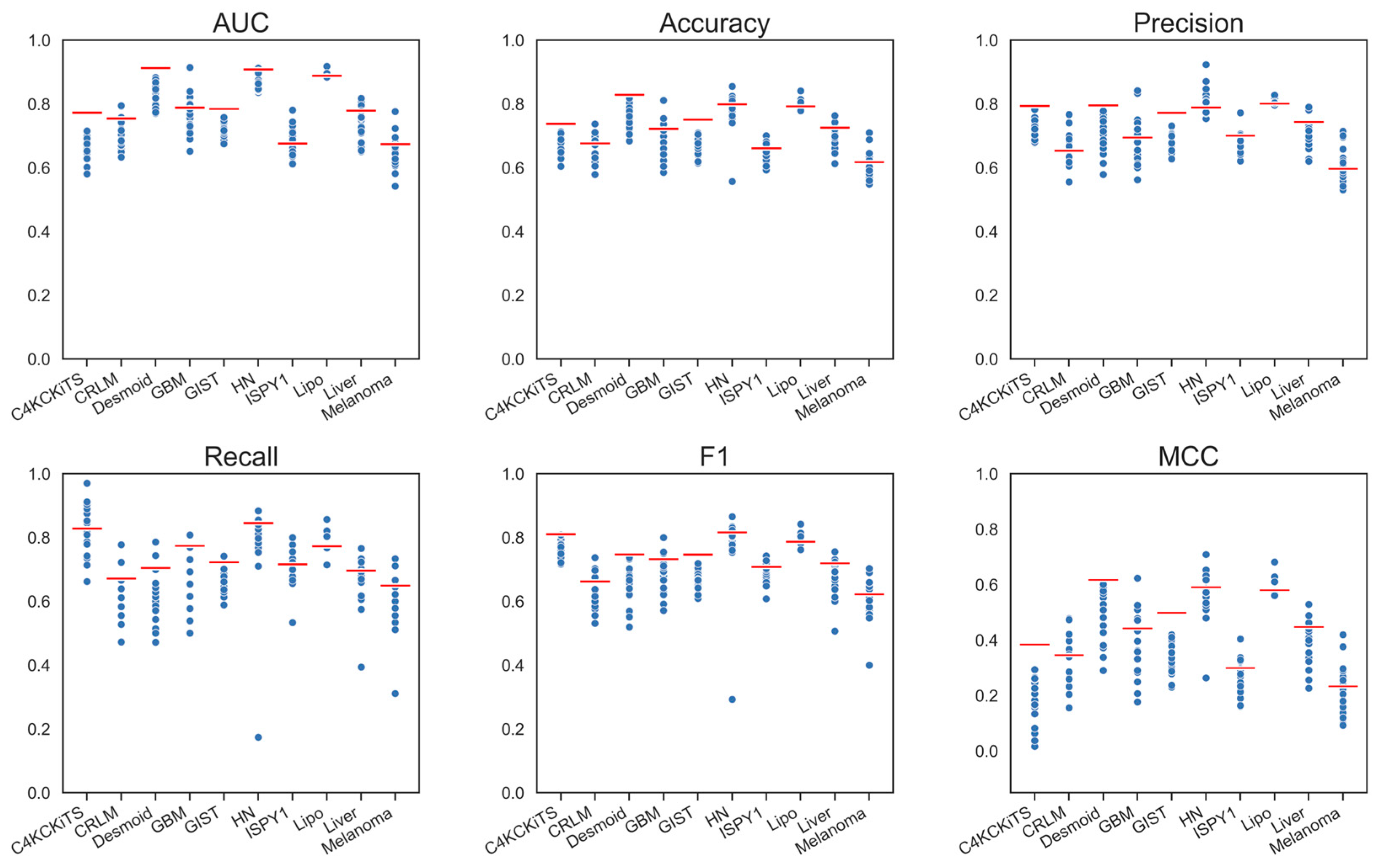
4.1. Hand-Crafted Features
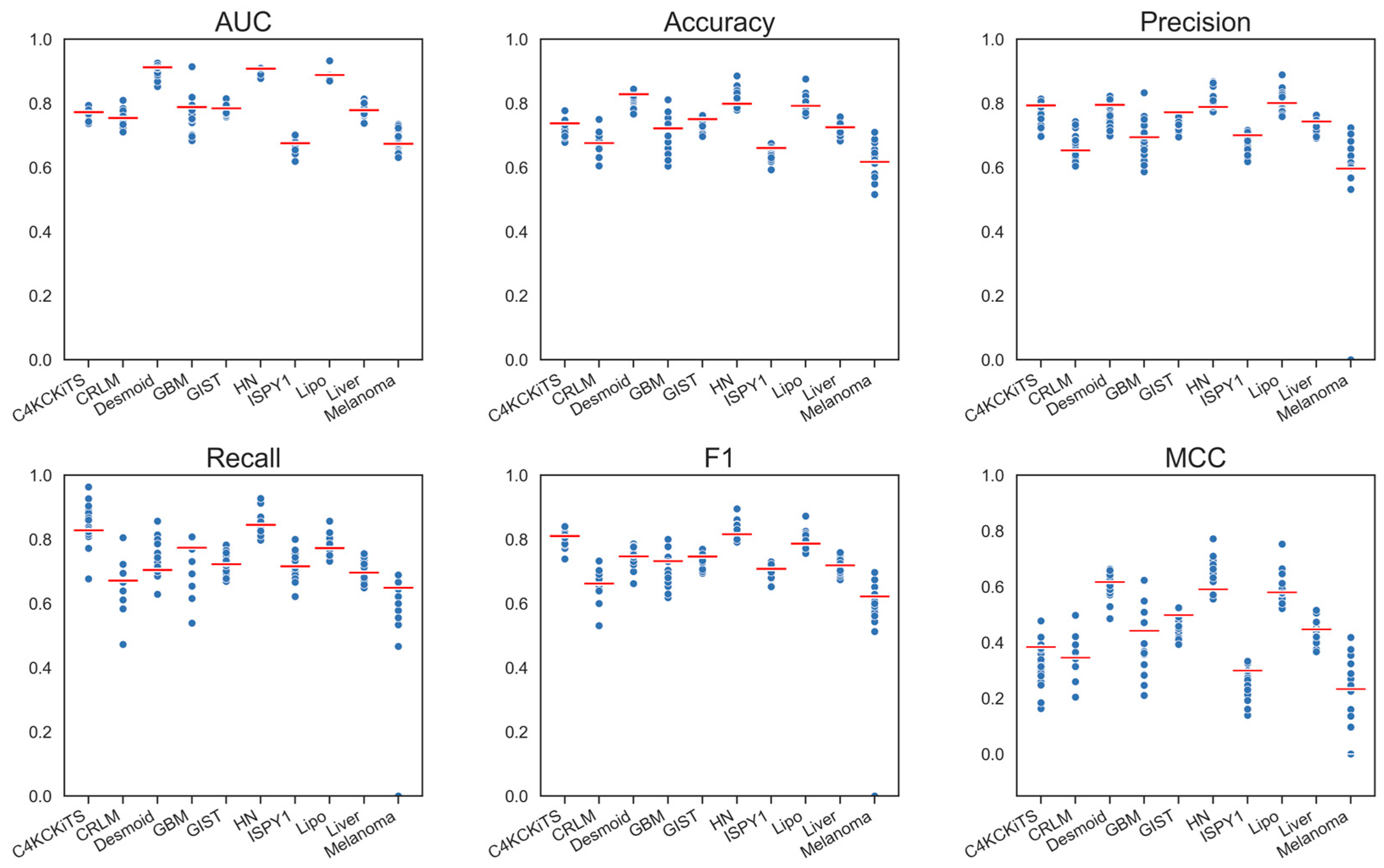
4.2. Deep Features
4.3. Deep Features Fused with Morphological Features
4.4. Deep Models Fused with All Hand-Crafted Features
5. Discussion
6. Future Work and Conclusions
Supplementary Materials
Funding
Institutional Review Board Statement
Informed Consent Statement
Data Availability Statement
Conflicts of Interest
References
- Lambin, P.; Rios-Velazquez, E.; Leijenaar, R.; Carvalho, S.; van Stiphout, R.G.P.M.; Granton, P.; Zegers, C.M.L.; Gillies, R.; Boellard, R.; Dekker, A.; et al. Radiomics: Extracting More Information from Medical Images Using Advanced Feature Analysis. Eur. J. Cancer 2012, 48, 441–446. [Google Scholar] [CrossRef] [PubMed]
- Kumar, V.; Gu, Y.; Basu, S.; Berglund, A.; Eschrich, S.A.; Schabath, M.B.; Forster, K.; Aerts, H.J.W.L.; Dekker, A.; Fenstermacher, D.; et al. Radiomics: The Process and the Challenges. Magn. Reson. Imaging 2012, 30, 1234–1248. [Google Scholar] [CrossRef] [PubMed]
- Mayerhoefer, M.E.; Materka, A.; Langs, G.; Häggström, I.; Szczypiński, P.; Gibbs, P.; Cook, G. Introduction to Radiomics. J. Nucl. Med. 2020, 61, 488–495. [Google Scholar] [CrossRef] [PubMed]
- Scapicchio, C.; Gabelloni, M.; Barucci, A.; Cioni, D.; Saba, L.; Neri, E. A Deep Look into Radiomics. Radiol. Med. 2021, 126, 1296–1311. [Google Scholar] [CrossRef]
- Harlow, C.A.; Dwyer, S.J.; Lodwick, G. On Radiographic Image Analysis. In Digital Picture Analysis; Springer: Berlin/Heidelberg, Germany, 1976; pp. 65–150. [Google Scholar]
- Haralick, R.M.; Shanmugam, K.; Dinstein, I. Textural Features for Image Classification. IEEE Trans. Syst. Man Cybern. 1973, SMC-3, 610–621. [Google Scholar] [CrossRef]
- Sun, C.; Wee, W.G. Neighboring Gray Level Dependence Matrix for Texture Classification. Comput. Vis. Graph. Image Process. 1983, 23, 341–352. [Google Scholar] [CrossRef]
- Miotto, R.; Wang, F.; Wang, S.; Jiang, X.; Dudley, J.T. Deep Learning for Healthcare: Review, Opportunities and Challenges. Brief. Bioinform. 2018, 19, 1236–1246. [Google Scholar] [CrossRef]
- Shen, D.; Wu, G.; Suk, H.-I. Deep Learning in Medical Image Analysis. Annu. Rev. Biomed. Eng. 2017, 19, 221–248. [Google Scholar] [CrossRef]
- LeCun, Y.; Bengio, Y.; Hinton, G. Deep Learning. Nature 2015, 521, 436–444. [Google Scholar] [CrossRef]
- Deng, J.; Dong, W.; Socher, R.; Li, L.-J.; Li, K.; Li, F.-F. ImageNet: A Large-Scale Hierarchical Image Database. In Proceedings of the 2009 IEEE Conference on Computer Vision and Pattern Recognition, Miami, FL, USA, 20–25 June 2009; pp. 248–255. [Google Scholar]
- Yan, L.; Yao, H.; Long, R.; Wu, L.; Xia, H.; Li, J.; Liu, Z.; Liang, C. A Preoperative Radiomics Model for the Identification of Lymph Node Metastasis in Patients with Early-Stage Cervical Squamous Cell Carcinoma. BJR 2020, 93, 20200358. [Google Scholar] [CrossRef]
- Aonpong, P.; Iwamoto, Y.; Han, X.-H.; Lin, L.; Chen, Y.-W. Improved Genotype-Guided Deep Radiomics Signatures for Recurrence Prediction of Non-Small Cell Lung Cancer. In Proceedings of the 2021 43rd Annual International Conference of the IEEE Engineering in Medicine & Biology Society (EMBC), Virtually, 1 November 2021; IEEE: Mexico City, Mexico, 2021; pp. 3561–3564. [Google Scholar]
- Bo, L.; Zhang, Z.; Jiang, Z.; Yang, C.; Huang, P.; Chen, T.; Wang, Y.; Yu, G.; Tan, X.; Cheng, Q.; et al. Differentiation of Brain Abscess from Cystic Glioma Using Conventional MRI Based on Deep Transfer Learning Features and Hand-Crafted Radiomics Features. Front. Med. 2021, 8, 748144. [Google Scholar] [CrossRef] [PubMed]
- Hou, Y.; Bao, J.; Song, Y.; Bao, M.-L.; Jiang, K.-W.; Zhang, J.; Yang, G.; Hu, C.-H.; Shi, H.-B.; Wang, X.-M.; et al. Integration of Clinicopathologic Identification and Deep Transferrable Image Feature Representation Improves Predictions of Lymph Node Metastasis in Prostate Cancer. EBioMedicine 2021, 68, 103395. [Google Scholar] [CrossRef]
- Yang, Y.; Wang, M.; Qiu, K.; Wang, Y.; Ma, X. Computed Tomography-Based Deep-Learning Prediction of Induction Chemotherapy Treatment Response in Locally Advanced Nasopharyngeal Carcinoma. Strahlenther. Onkol. 2022, 198, 183–193. [Google Scholar] [CrossRef] [PubMed]
- Yang, Y.; Zhou, Y.; Zhou, C.; Ma, X. Deep Learning Radiomics Based on Contrast Enhanced Computed Tomography Predicts Microvascular Invasion and Survival Outcome in Early Stage Hepatocellular Carcinoma. Eur. J. Surg. Oncol. 2022, 48, 1068–1077. [Google Scholar] [CrossRef]
- Zhu, Y.; Man, C.; Gong, L.; Dong, D.; Yu, X.; Wang, S.; Fang, M.; Wang, S.; Fang, X.; Chen, X.; et al. A Deep Learning Radiomics Model for Preoperative Grading in Meningioma. Eur. J. Radiol. 2019, 116, 128–134. [Google Scholar] [CrossRef] [PubMed]
- Feng, B.; Chen, X.; Chen, Y.; Lu, S.; Liu, K.; Li, K.; Liu, Z.; Hao, Y.; Li, Z.; Zhu, Z.; et al. Solitary Solid Pulmonary Nodules: A CT-Based Deep Learning Nomogram Helps Differentiate Tuberculosis Granulomas from Lung Adenocarcinomas. Eur. Radiol. 2020, 30, 6497–6507. [Google Scholar] [CrossRef]
- Ziegelmayer, S.; Kaissis, G.; Harder, F.; Jungmann, F.; Müller, T.; Makowski, M.; Braren, R. Deep Convolutional Neural Network-Assisted Feature Extraction for Diagnostic Discrimination and Feature Visualization in Pancreatic Ductal Adenocarcinoma (PDAC) versus Autoimmune Pancreatitis (AIP). J. Clin. Med. 2020, 9, 4013. [Google Scholar] [CrossRef]
- Fu, J.; Zhong, X.; Li, N.; Dams, R.V.; Lewis, J.; Sung, K.; Raldow, A.C.; Jin, J.; Qi, X.S. Deep Learning-Based Radiomic Features for Improving Neoadjuvant Chemoradiation Response Prediction in Locally Advanced Rectal Cancer. Phys. Med. Biol. 2020, 65, 075001. [Google Scholar] [CrossRef]
- Zwanenburg, A.; Vallières, M.; Abdalah, M.A.; Aerts, H.J.W.L.; Andrearczyk, V.; Apte, A.; Ashrafinia, S.; Bakas, S.; Beukinga, R.J.; Boellaard, R.; et al. The Image Biomarker Standardization Initiative: Standardized Quantitative Radiomics for High-Throughput Image-Based Phenotyping. Radiology 2020, 295, 328–338. [Google Scholar] [CrossRef]
- Castaldo, R.; Pane, K.; Nicolai, E.; Salvatore, M.; Franzese, M. The Impact of Normalization Approaches to Automatically Detect Radiogenomic Phenotypes Characterizing Breast Cancer Receptors Status. Cancers 2020, 12, 518. [Google Scholar] [CrossRef]
- Hu, Y.; Xie, C.; Yang, H.; Ho, J.W.K.; Wen, J.; Han, L.; Lam, K.-O.; Wong, I.Y.H.; Law, S.Y.K.; Chiu, K.W.H.; et al. Computed Tomography-Based Deep-Learning Prediction of Neoadjuvant Chemoradiotherapy Treatment Response in Esophageal Squamous Cell Carcinoma. Radiother. Oncol. 2021, 154, 6–13. [Google Scholar] [CrossRef] [PubMed]
- Xuan, R.; Li, T.; Wang, Y.; Xu, J.; Jin, W. Prenatal Prediction and Typing of Placental Invasion Using MRI Deep and Radiomic Features. BioMed Eng. OnLine 2021, 20, 56. [Google Scholar] [CrossRef]
- Bertelli, E.; Mercatelli, L.; Marzi, C.; Pachetti, E.; Baccini, M.; Barucci, A.; Colantonio, S.; Gherardini, L.; Lattavo, L.; Pascali, M.A.; et al. Machine and Deep Learning Prediction of Prostate Cancer Aggressiveness Using Multiparametric MRI. Front. Oncol. 2022, 11, 802964. [Google Scholar] [CrossRef]
- Kocak, B.; Baessler, B.; Bakas, S.; Cuocolo, R.; Fedorov, A.; Maier-Hein, L.; Mercaldo, N.; Müller, H.; Orlhac, F.; Pinto dos Santos, D.; et al. CheckList for EvaluAtion of Radiomics Research (CLEAR): A Step-by-Step Reporting Guideline for Authors and Reviewers Endorsed by ESR and EuSoMII. Insights Into Imaging 2023, 14, 75. [Google Scholar] [CrossRef] [PubMed]
- Kocak, B. Key Concepts, Common Pitfalls, and Best Practices in Artificial Intelligence and Machine Learning: Focus on Radiomics. Diagn. Interv. Radiol. 2022, 28, 450–462. [Google Scholar] [CrossRef] [PubMed]
- Starmans, M.P.A.; Timbergen, M.J.M.; Vos, M.; Padmos, G.A.; Grünhagen, D.J.; Verhoef, C.; Sleijfer, S.; van Leenders, G.J.L.H.; Buisman, F.E.; Willemssen, F.E.J.A.; et al. The WORC Database: MRI and CT Scans, Segmentations, and Clinical Labels for 930 Patients from Six Radiomics Studies. medRxiv 2021, preprint. [Google Scholar]
- Clark, K.; Vendt, B.; Smith, K.; Freymann, J.; Kirby, J.; Koppel, P.; Moore, S.; Phillips, S.; Maffitt, D.; Pringle, M.; et al. The Cancer Imaging Archive (TCIA): Maintaining and Operating a Public Information Repository. J. Digit. Imaging 2013, 26, 1045–1057. [Google Scholar] [CrossRef]
- Heller, N.; Sathianathen, N.; Kalapara, A.; Walczak, E.; Moore, K.; Kaluzniak, H.; Rosenberg, J.; Blake, P.; Rengel, Z.; Oestreich, M.; et al. The KiTS19 Challenge Data: 300 Kidney Tumor Cases with Clinical Context, CT Semantic Segmentations, and Surgical Outcomes. arXiv 2020, arXiv:1904.00445. [Google Scholar]
- Scarpace, L.; Mikkelsen, T.; Cha, S.; Rao, S.; Tekchandani, S.; Gutman, D.; Saltz, J.H.; Erickson, B.J.; Pedano, N.; Flanders, A.E.; et al. Radiology Data from The Cancer Genome Atlas Glioblastoma Multiforme [TCGA-GBM] Collection 2016. Available online: https://wiki.cancerimagingarchive.net/pages/viewpage.action?pageId=1966258 (accessed on 31 July 2023).
- Aerts, H.J.W.L.; Velazquez, E.R.; Leijenaar, R.T.H.; Parmar, C.; Grossmann, P.; Carvalho, S.; Bussink, J.; Monshouwer, R.; Haibe-Kains, B.; Rietveld, D.; et al. Decoding Tumour Phenotype by Noninvasive Imaging Using a Quantitative Radiomics Approach. Nat. Commun. 2014, 5, 4006. [Google Scholar] [CrossRef]
- Hylton, N.M.; Gatsonis, C.A.; Rosen, M.A.; Lehman, C.D.; Newitt, D.C.; Partridge, S.C.; Bernreuter, W.K.; Pisano, E.D.; Morris, E.A.; Weatherall, P.T.; et al. Neoadjuvant Chemotherapy for Breast Cancer: Functional Tumor Volume by MR Imaging Predicts Recurrence-Free Survival—Results from the ACRIN 6657/CALGB 150007 I-SPY 1 TRIAL. Radiology 2015, 279, 44–55. [Google Scholar] [CrossRef]
- van Griethuysen, J.J.M.; Fedorov, A.; Parmar, C.; Hosny, A.; Aucoin, N.; Narayan, V.; Beets-Tan, R.G.H.; Fillion-Robin, J.-C.; Pieper, S.; Aerts, H.J.W.L. Computational Radiomics System to Decode the Radiographic Phenotype. Cancer Res. 2017, 77, e104–e107. [Google Scholar] [CrossRef] [PubMed]
- Demircioğlu, A. Predictive Performance of Radiomic Models Based on Features Extracted from Pretrained Deep Networks. Insights Imaging 2022, 13, 187. [Google Scholar] [CrossRef]
- He, K.; Zhang, X.; Ren, S.; Sun, J. Deep Residual Learning for Image Recognition. In Proceedings of the 2016 IEEE Conference on Computer Vision and Pattern Recognition (CVPR), Las Vegas, NV, USA, 27–30 June 2016; pp. 770–778. [Google Scholar]
- Huang, G.; Liu, Z.; van der Maaten, L.; Weinberger, K.Q. Densely Connected Convolutional Networks. arXiv 2016, arXiv:1608.06993. [Google Scholar]
- Simonyan, K.; Zisserman, A. Very Deep Convolutional Networks for Large-Scale Image Recognition. arXiv 2015, arXiv:1409.1556. [Google Scholar]
- Szegedy, C.; Vanhoucke, V.; Ioffe, S.; Shlens, J.; Wojna, Z. Rethinking the Inception Architecture for Computer Vision. In Proceedings of the 2016 IEEE Conference on Computer Vision and Pattern Recognition (CVPR), Las Vegas, NV, USA, 27–30 June 2016; pp. 2818–2826. [Google Scholar]
- Mei, X.; Liu, Z.; Robson, P.M.; Marinelli, B.; Huang, M.; Doshi, A.; Jacobi, A.; Cao, C.; Link, K.E.; Yang, T.; et al. RadImageNet: An Open Radiologic Deep Learning Research Dataset for Effective Transfer Learning. Radiol. Artif. Intell. 2022, 4, e210315. [Google Scholar] [CrossRef] [PubMed]
- Chen, S.; Ma, K.; Zheng, Y. Med3D: Transfer Learning for 3D Medical Image Analysis. arXiv 2019, arXiv:1904.00625. [Google Scholar]
- Woo, S.; Debnath, S.; Hu, R.; Chen, X.; Liu, Z.; Kweon, I.S.; Xie, S. ConvNeXt V2: Co-Designing and Scaling ConvNets with Masked Autoencoders. arXiv 2023, arXiv:2301.00808. [Google Scholar]
- Touvron, H.; Cord, M.; Jégou, H. DeiT III: Revenge of the ViT. arXiv 2022, arXiv:2204.07118. [Google Scholar]
- Tan, M.; Le, Q.V. EfficientNet: Rethinking Model Scaling for Convolutional Neural Networks. arXiv 2019, arXiv:1905.11946. [Google Scholar]
- Tan, M.; Le, Q.V. EfficientNetV2: Smaller Models and Faster Training. arXiv 2021, arXiv:2104.00298. [Google Scholar]
- Chen, T.; Kornblith, S.; Norouzi, M.; Hinton, G. A Simple Framework for Contrastive Learning of Visual Representations. arXiv 2020, arXiv:2002.05709. [Google Scholar]
- Chen, X.; He, K. Exploring Simple Siamese Representation Learning. arXiv 2020, arXiv:2011.10566. [Google Scholar]
- Chen, X.; Xie, S.; He, K. An Empirical Study of Training Self-Supervised Vision Transformers. arXiv 2021, arXiv:2104.02057. [Google Scholar]
- Zbontar, J.; Jing, L.; Misra, I.; LeCun, Y.; Deny, S. Barlow Twins: Self-Supervised Learning via Redundancy Reduction. arXiv 2021, arXiv:2103.03230. [Google Scholar]
- Demircioğlu, A. Benchmarking Feature Selection Methods in Radiomics. Investig. Radiol. 2022. ahead of print. [Google Scholar] [CrossRef] [PubMed]
- Taha, A.A.; Hanbury, A. Metrics for Evaluating 3D Medical Image Segmentation: Analysis, Selection, and Tool. BMC Med. Imaging 2015, 15, 29. [Google Scholar] [CrossRef] [PubMed]
- Chicco, D.; Jurman, G. The Advantages of the Matthews Correlation Coefficient (MCC) over F1 Score and Accuracy in Binary Classification Evaluation. BMC Genom. 2020, 21, 6. [Google Scholar] [CrossRef]
- Ger, R.B.; Zhou, S.; Elgohari, B.; Elhalawani, H.; Mackin, D.M.; Meier, J.G.; Nguyen, C.M.; Anderson, B.M.; Gay, C.; Ning, J.; et al. Radiomics Features of the Primary Tumor Fail to Improve Prediction of Overall Survival in Large Cohorts of CT- and PET-Imaged Head and Neck Cancer Patients. PLoS ONE 2019, 14, e0222509. [Google Scholar] [CrossRef]
- Berisha, V.; Krantsevich, C.; Hahn, P.R.; Hahn, S.; Dasarathy, G.; Turaga, P.; Liss, J. Digital Medicine and the Curse of Dimensionality. NPJ Digit. Med. 2021, 4, 153. [Google Scholar] [CrossRef]
- Wolpert, D.H. The Lack of A Priori Distinctions Between Learning Algorithms. Neural Comput. 1996, 8, 1341–1390. [Google Scholar] [CrossRef]
- Ziegelmayer, S.; Reischl, S.; Harder, F.; Makowski, M.; Braren, R.; Gawlitza, J. Feature Robustness and Diagnostic Capabilities of Convolutional Neural Networks Against Radiomics Features in Computed Tomography Imaging. Investig. Radiol. 2022, 57, 171–177. [Google Scholar] [CrossRef] [PubMed]
- Demircioğlu, A. Are Deep Models in Radiomics Performing Better than Generic Models? A Systematic Review. Eur. Radiol. Exp. 2023, 7, 11. [Google Scholar] [CrossRef] [PubMed]
- Wainer, J.; Cawley, G. Nested Cross-Validation When Selecting Classifiers Is Overzealous for Most Practical Applications. Expert Syst. Appl. 2021, 182, 115222. [Google Scholar] [CrossRef]

| Study | Year | Pathology | Modality | AUC (Hand-Crafted) | AUC (Deep) | ΔAUC |
|---|---|---|---|---|---|---|
| Zhu et al. [18] | 2019 | Brain cancer | MR | 0.68 | 0.81 | 0.13 |
| Feng et al. [19] | 2020 | Lung cancer | CT | 0.7 | 0.8 | 0.1 |
| Fu et al. [21] | 2020 | Rectal cancer | MR | 0.64 | 0.73 | 0.09 |
| Yan et al. [12] | 2020 | Cervical cancer | MR | 0.72 | 0.72 | 0.0 |
| Ziegelmayer et al. [20] | 2020 | Pancreatic cancer | CT | 0.8 | 0.9 | 0.1 |
| Aonpong et al. [13] | 2021 | Lung cancer | CT | 0.68 | 0.69 | 0.01 |
| Bo et al. [14] | 2021 | Brain cancer | MR | 0.75 | 0.71 | −0.04 |
| Hou et al. [15] | 2021 | Prostate cancer | MR | 0.83 | 0.84 | 0.01 |
| Hu et al. [24] | 2021 | Lung cancer | CT | 0.82 | 0.9 | 0.08 |
| Xuan et al. [25] | 2021 | Placenta invasion | MR | 0.8 | 0.88 | 0.08 |
| Bertelli et al. [26] | 2022 | Prostate cancer | MR | 0.8 | 0.85 | 0.05 |
| Yang et al. [16] | 2022 | Head and neck cancer | CT | 0.66 | 0.81 | 0.15 |
| Yang et al. [17] | 2022 | Liver cancer | CT | 0.74 | 0.88 | 0.14 |
| Dataset | Modality (Weighting) | Sample Size (n) | Size of Minor Class | Size of Major Class | Class Balance | In-Plane Resolution [mm] | Slice Thickness [mm] | Source |
|---|---|---|---|---|---|---|---|---|
| C4KC-KiTS | CT | 203 | 67 | 142 | 2.12 | 0.8 (0.4–1.0) | 3.0 (1.0–5.0) | TCIA [31] |
| CRLM | CT | 76 | 36 | 40 | 1.11 | 0.7 (0.6–0.9) | 5.0 (1.0–8.0) | WORC [29] |
| Desmoid | MR (T1) | 195 | 71 | 125 | 1.76 | 0.7 (0.2–1.8) | 5.0 (1.0–10.0) | WORC [29] |
| GBM | MR (T1) | 53 | 26 | 27 | 1.04 | 0.7 (0.6–0.9) | 5.0 (1.0–8.0) | TCIA [32] |
| GIST | CT | 244 | 120 | 125 | 1.04 | 0.8 (0.6–1.0) | 3.0 (0.6–6.0) | WORC [29] |
| HN | CT | 134 | 65 | 69 | 1.06 | 1.0 (1.0–1.1) | 3.0 (1.5–3.0) | TCIA [33] |
| ISPY-1 | MR (DCE) | 157 | 69 | 92 | 1.33 | 0.8 (0.4–1.2) | 2.1 (1.5–3.4) | TCIA [34] |
| Lipo | MR (T1) | 113 | 57 | 57 | 1 | 0.7 (0.2–1.4) | 5.5 (1.0–9.1) | WORC [29] |
| Liver | MR (T2) | 186 | 92 | 94 | 1.02 | 0.8 (0.6–1.6) | 7.7 (1.0–11.0) | WORC [29] |
| Melanoma | CT | 97 | 48 | 49 | 1.02 | 0.8 (0.4–1.0) | 3.0 (1.0–5.0) | WORC [29] |
| Model | AUC | ΔAUC | Accuracy | ΔAccuracy | ΔRecall | Recall | Precision | ΔPrecision | MCC | ΔMCC | F1 | ΔF1 |
|---|---|---|---|---|---|---|---|---|---|---|---|---|
| Hand-Crafted Features | ||||||||||||
| Hand-crafted, 2-D, All | 0.794 | 0.005 | 0.727 | 0.001 | 0.766 | 0.033 | 0.716 | −0.013 | 0.441 | 0.002 | 0.74 | 0.01 |
| Hand-crafted, 2-D, No morph | 0.793 | 0.004 | 0.735 | 0.009 | 0.741 | 0.008 | 0.738 | 0.009 | 0.456 | 0.017 | 0.737 | 0.007 |
| Hand-crafted, 3-D, No morph | 0.791 | 0.002 | 0.733 | 0.007 | 0.732 | −0.001 | 0.738 | 0.009 | 0.454 | 0.015 | 0.734 | 0.004 |
| Hand-crafted, 3-D, All | 0.789 | - | 0.726 | - | 0.733 | - | 0.729 | - | 0.439 | - | 0.73 | - |
| Hand-crafted, 3-D, Morph | 0.723 | −0.066 | 0.663 | −0.063 | 0.618 | −0.115 | 0.698 | −0.031 | 0.303 | −0.136 | 0.627 | −0.103 |
| Deep Features | ||||||||||||
| ConvNeXt V2, large | 0.775 | −0.014 | 0.708 | −0.018 | 0.718 | −0.015 | 0.709 | −0.02 | 0.402 | −0.037 | 0.712 | −0.018 |
| SimSiam, ResNet-50 | 0.766 | −0.023 | 0.704 | −0.022 | 0.711 | −0.022 | 0.704 | −0.025 | 0.385 | −0.054 | 0.699 | −0.031 |
| SimCLR, ResNet-50 | 0.761 | −0.028 | 0.709 | −0.017 | 0.745 | 0.012 | 0.701 | −0.028 | 0.391 | −0.048 | 0.72 | −0.01 |
| Deep and Morphological Features | ||||||||||||
| ConvNeXt V2, large | 0.778 | −0.011 | 0.714 | −0.012 | 0.724 | −0.009 | 0.717 | −0.012 | 0.412 | −0.027 | 0.72 | −0.01 |
| SimSiam, ResNet-50 | 0.777 | −0.012 | 0.714 | −0.012 | 0.745 | 0.012 | 0.707 | −0.022 | 0.4 | −0.039 | 0.723 | −0.007 |
| EfficientNet-B2 | 0.773 | −0.016 | 0.716 | −0.01 | 0.708 | −0.025 | 0.73 | 0.001 | 0.416 | −0.023 | 0.715 | −0.015 |
| Deep and All Hand-Crafted Features | ||||||||||||
| SimSiam, ResNet-50 | 0.798 | 0.009 | 0.734 | 0.008 | 0.727 | −0.006 | 0.737 | 0.008 | 0.45 | 0.011 | 0.731 | 0.001 |
| EfficientNet V2, large | 0.795 | 0.006 | 0.719 | −0.007 | 0.683 | −0.05 | 0.669 | −0.06 | 0.414 | −0.025 | 0.674 | −0.056 |
| EfficientNet-B2 | 0.795 | 0.006 | 0.739 | 0.013 | 0.758 | 0.025 | 0.738 | 0.009 | 0.464 | 0.025 | 0.747 | 0.017 |
Disclaimer/Publisher’s Note: The statements, opinions and data contained in all publications are solely those of the individual author(s) and contributor(s) and not of MDPI and/or the editor(s). MDPI and/or the editor(s) disclaim responsibility for any injury to people or property resulting from any ideas, methods, instructions or products referred to in the content. |
© 2023 by the author. Licensee MDPI, Basel, Switzerland. This article is an open access article distributed under the terms and conditions of the Creative Commons Attribution (CC BY) license (https://creativecommons.org/licenses/by/4.0/).
Share and Cite
Demircioğlu, A. Deep Features from Pretrained Networks Do Not Outperform Hand-Crafted Features in Radiomics. Diagnostics 2023, 13, 3266. https://doi.org/10.3390/diagnostics13203266
Demircioğlu A. Deep Features from Pretrained Networks Do Not Outperform Hand-Crafted Features in Radiomics. Diagnostics. 2023; 13(20):3266. https://doi.org/10.3390/diagnostics13203266
Chicago/Turabian StyleDemircioğlu, Aydin. 2023. "Deep Features from Pretrained Networks Do Not Outperform Hand-Crafted Features in Radiomics" Diagnostics 13, no. 20: 3266. https://doi.org/10.3390/diagnostics13203266
APA StyleDemircioğlu, A. (2023). Deep Features from Pretrained Networks Do Not Outperform Hand-Crafted Features in Radiomics. Diagnostics, 13(20), 3266. https://doi.org/10.3390/diagnostics13203266