
Skeleton Segmentation on Bone Scintigraphy for BSI Computation


Abstract
1. Introduction
2. Materials and Methods
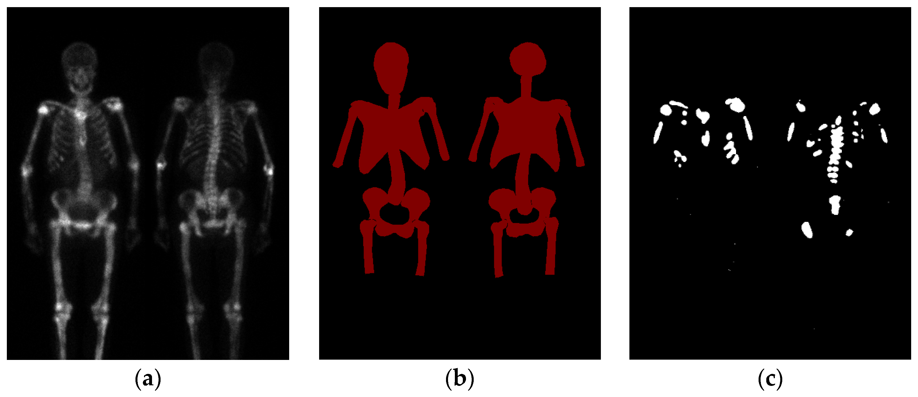
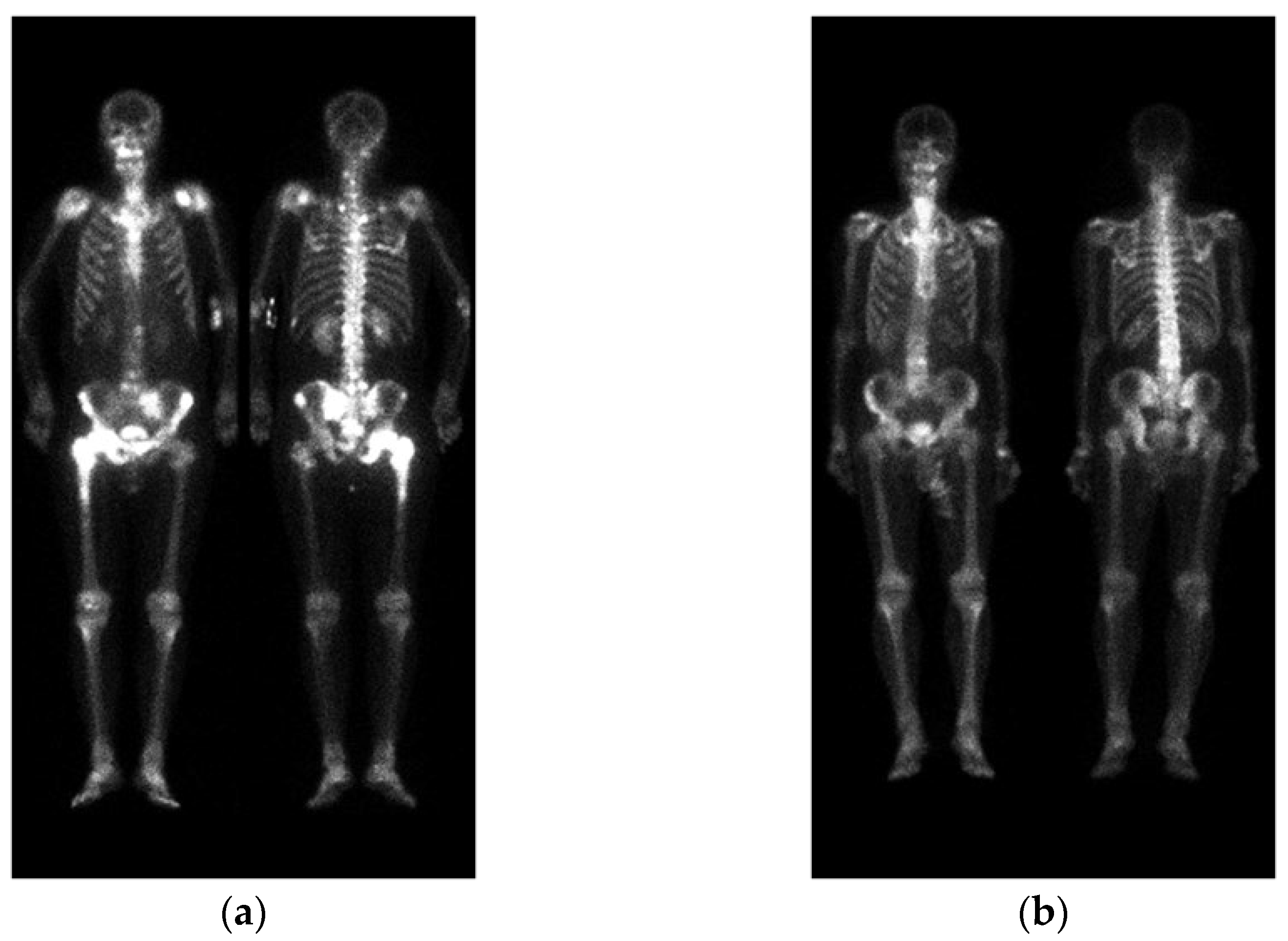
2.1. Materials
2.2. Region Definition
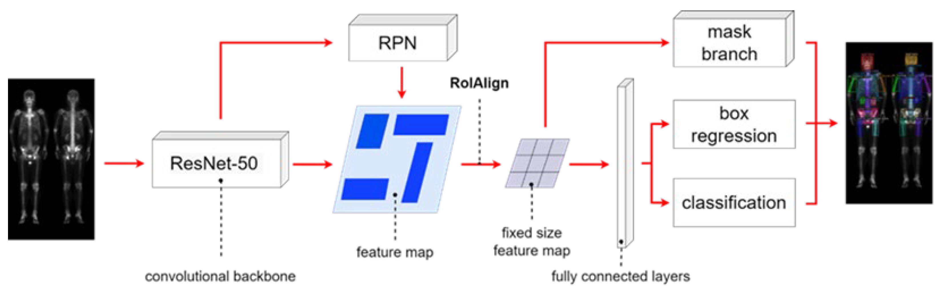
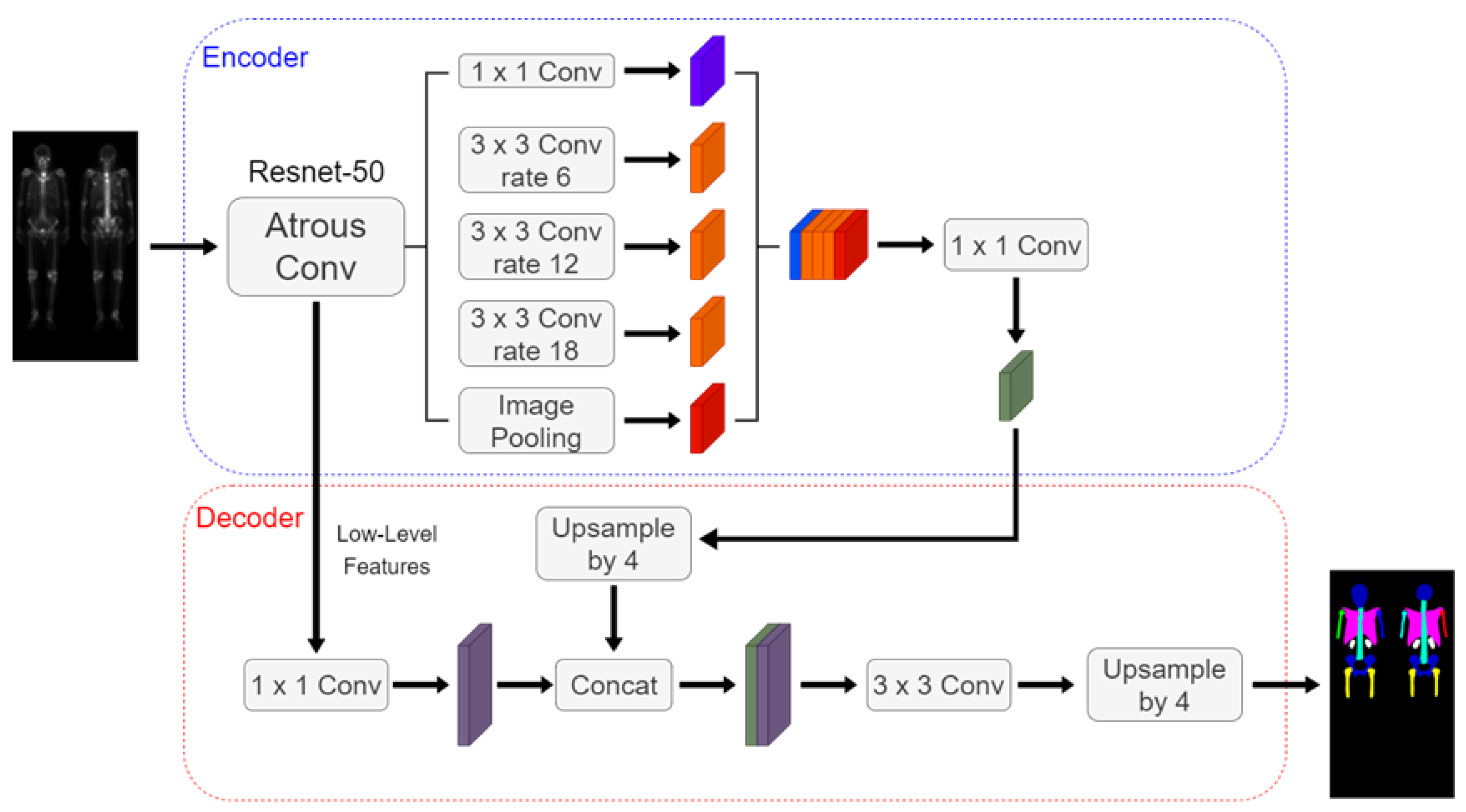
2.3. Neural Network Architectures
2.4. Image Pre-Processing
2.5. Evaluations
3. Results
3.1. 10-Fold Cross-Validation
3.2. 10-Fold Cross-Validation with Data Augmentation
4. Discussion
5. Conclusions
Author Contributions
Funding
Institutional Review Board Statement
Informed Consent Statement
Data Availability Statement
Acknowledgments
Conflicts of Interest
Appendix A
References
- Coleman, R. Metastatic bone disease: Clinical features, pathophysiology, and treatment strategies. Cancer Treat. Rev. 2001, 27, 165–176. [Google Scholar] [CrossRef] [PubMed]
- National Health Insurance Research Database. Available online: https://www.mohw.gov.tw/cp-16-70314-1.html (accessed on 12 May 2022).
- O’Sullivan, G.J.; Carty, F.L.; Cronin, C.G. Imaging of bone metastasis: An update. World J. Radiol. 2015, 7, 202–211. [Google Scholar] [CrossRef]
- Coleman, R.E. Clinical features of metastatic bone disease and risk of skeletal morbidity. Clin. Cancer Res. 2006, 12, 6243–6249. [Google Scholar] [CrossRef] [PubMed]
- Brenner, A.I.; Koshy, J.; Morey, J.; Lin, C.; DiPoce, J. The bone scan. Semin. Nucl. Med. 2012, 42, 11–26. [Google Scholar] [CrossRef]
- Imbriaco, M.; Larson, S.M.; Yeung, H.W.; Mawlawi, O.R.; Erdi, Y.; Venkatraman, E.S.; Scher, H.I. A new parameter for measuring metastatic bone involvement by prostate cancer: The Bone Scan Index. Clin. Cancer Res. Off. J. Am. Assoc. Cancer Res. 1998, 4, 1765–1772. [Google Scholar]
- Dennis, E.R.; Jia, X.; Mezheritskiy, I.S.; Stephenson, R.D.; Schoder, H.; Fox, J.J.; Heller, G.; Scher, H.I.; Larson, S.M.; Morris, M.J. Bone scan index: A quantitative treatment response biomarker for castration-resistant metastatic prostate cancer. J. Clin. Oncol. 2012, 30, 519–524. [Google Scholar] [CrossRef] [PubMed]
- Anand, A.; Morris, M.J.; Kaboteh, R.; Båth, L.; Sadik, M.; Gjertsson, P.; Lomsky, M.; Edenbrandt, L.; Minarik, D.; Bjartell, A. Analytic validation of the automated bone scan index as an imaging biomarker to standardize quantitative changes in bone scans of patients with metastatic prostate cancer. J. Nucl. Med. 2016, 57, 41–45. [Google Scholar] [CrossRef]
- Nakajima, K.; Edenbrandt, L.; Mizokami, A. Bone scan index: A new biomarker of bone metastasis in patients with prostate cancer. Int. J. Urol. 2017, 24, 668–673. [Google Scholar] [CrossRef]
- Armstrong, A.J.; Nordle, O.; Morris, M. Assessing the Prognostic Value of the Automated Bone Scan Index for Prostate Cancer—Reply. JAMA Oncol. 2019, 5, 270–271. [Google Scholar] [CrossRef]
- Ulmert, D.; Kaboteh, R.; Fox, J.J.; Savage, C.; Evans, M.J.; Lilja, H.; Abrahamsson, P.A.; Björk, T.; Gerdtsson, A.; Bjartell, A.; et al. A novel automated platform for quantifying the extent of skeletal tumour involvement in prostate cancer patients using the Bone Scan Index. Eur. Urol. 2012, 62, 78–84. [Google Scholar] [CrossRef]
- Reza, M.; Kaboteh, R.; Sadik, M.; Bjartell, A.; Wollmer, P.; Trägårdh, E. A prospective study to evaluate the intra-individual reproducibility of bone scans for quantitative assessment in patients with metastatic prostate cancer. BMC Med. Imaging 2018, 18, 8. [Google Scholar] [CrossRef] [PubMed]
- Armstrong, A.J.; Anand, A.; Edenbrandt, L.; Bondesson, E.; Bjartell, A.; Widmark, A.; Sternberg, C.N.; Pili, R.; Tuvesson, H.; Nordle, O. Phase 3 assessment of the automated bone scan index as a prognostic imaging biomarker of overall survival in men with metastatic castration-resistant prostate cancer: A secondary analysis of a randomized clinical trial. JAMA Oncol. 2018, 4, 944–951. [Google Scholar] [CrossRef] [PubMed]
- Anand, A.; Morris, M.J.; Kaboteh, R.; Reza, M.; Trägårdh, E.; Matsunaga, N.; Edenbrandt, L.; Bjartell, A.; Larson, S.M.; Minarik, D. A preanalytic validation study of automated bone scan index: Effect on accuracy and reproducibility due to the procedural variabilities in bone scan image acquisition. J. Nucl. Med. 2016, 57, 1865–1871. [Google Scholar] [CrossRef] [PubMed]
- Reza, M.; Wirth, M.; Tammela, T.; Cicalese, V.; Veiga, F.G.; Mulders, P.; Miller, K.; Tubaro, A.; Debruyne, F.; Patel, A.; et al. Automated bone scan index as an imaging biomarker to predict overall survival in the Zometa European Study/SPCG11. Eur. Urol. Oncol. 2021, 4, 49–55. [Google Scholar] [CrossRef]
- Wuestemann, J.; Hupfeld, S.; Kupitz, D.; Genseke, P.; Schenke, S.; Pech, M.; Kreissl, M.C.; Grosser, O.S. Analysis of bone scans in various tumor entities using a deep-learning-based artificial neural network algorithm—Evaluation of diagnostic performance. Cancers 2020, 12, 2654. [Google Scholar] [CrossRef]
- Yoshida, A.; Higashiyama, S.; Kawabe, J. Assessment of software for semi-automatically calculating the bone scan index on bone scintigraphy scans. Clin. Imaging 2021, 78, 14–18. [Google Scholar] [CrossRef]
- Koizumi, M.; Wagatsuma, K.; Miyaji, N.; Murata, T.; Miwa, K.; Takiguchi, T.; Makino, T.; Koyama, M. Evaluation of a computer-assisted diagnosis system, BONENAVI version 2, for bone scintigraphy in cancer patients in a routine clinical setting. Ann. Nucl. Med. 2015, 29, 138–148. [Google Scholar] [CrossRef]
- Koizumi, M.; Miyaji, N.; Murata, T.; Motegi, K.; Miwa, K.; Koyama, M.; Terauchi, T.; Wagatsuma, K.; Kawakami, K.; Richter, J. Evaluation of a revised version of the computer-assisted diagnosis system, BONENAVI version 2.1.7, for bone scintigraphy in cancer patients. Ann. Nucl. Med. 2015, 29, 659–665. [Google Scholar] [CrossRef]
- Shimizu, A.; Wakabayashi, H.; Kanamori, T.; Saito, A.; Nishikawa, K.; Daisaki, H.; Higashiyama, S.; Kawabe, J. Correction to: Automated measurement of bone scan index from a whole-body bone scintigram. Int. J. Comput.-Assist. Radiol. Surg. 2020, 15, 401. [Google Scholar] [CrossRef]
- Cheng, D.C.; Liu, C.C.; Hsieh, T.C.; Yen, K.Y.; Kao, C.H. Bone metastasis detection in the chest and pelvis from a whole-body bone scan using deep learning and a small dataset. Electronics 2021, 10, 1201. [Google Scholar] [CrossRef]
- Cheng, D.C.; Hsieh, T.C.; Yen, K.Y.; Kao, C.H. Lesion-based bone metastasis detection in chest bone scintigraphy images of prostate cancer patients using pre-train, negative mining, and deep learning. Diagnostics 2021, 11, 518. [Google Scholar] [CrossRef] [PubMed]
- Cheng, D.C.; Liu, C.C.; Kao, C.H.; Hsieh, T.C. System of Deep Learning Neural Network in Prostate Cancer Bone Metastasis Identification Based on Whole Body Bone Scan Images. U.S. Patent US11488303B2, 1 November 2022. [Google Scholar]
- Brown, M.S. Computer-Aided Bone Scan Assessment with Automated Lesion Detection and Quantitative Assessment of Bone Disease Burden Changes. U.S. Patent US20140105471, 7 April 2015. [Google Scholar]
- Huang, K.B.; Huang, S.G.; Chen, G.J.; Li, X.; Li, S.; Liang, Y.; Gao, Y. An end-to-end multi-task system of automatic lesion detection and anatomical localization in whole-body bone scintigraphy by deep learning. Bioinformatics 2023, 39, btac753. [Google Scholar] [CrossRef] [PubMed]
- He, K.; Gkioxari, G.; Dollár, P.; Girshick, R. Mask R-CNN. arXiv 2018, arXiv:1703.06870v3. [Google Scholar]
- Jha, D.; Riegler, M.A.; Johansen, D.; Halvorsen, P.; Johansen, H.D. Double U-Net: A Deep Convolutional Neural Network for Medical Image Segmentation. arXiv 2020, arXiv:2006.04868. [Google Scholar]
- Chen, L.C.; Zhu, Y.; Papandreou, G.; Schroff, F.; Adam, H. Encoder-Decoder with Atrous Separable Convolution for Semantic Image Segmentation. arXiv 2018, arXiv:1802.02611v3. [Google Scholar]
- Bhuse, P.; Singh, B.; Raut, P. Effect of data augmentation on the accuracy of convolutional neural networks. In Information and Communication Technology for Competitive Strategies (ICTCS 2020) ICT: Applications and Social Interfaces; Springer: Berlin/Heidelberg, Germany, 2020; pp. 337–348. [Google Scholar]


| Hyperparameters | Mask R-CNN | Double U-Net | DeeplabV3 Plus |
|---|---|---|---|
| Learning Rate | 0.005 | 0.0005 | 0.0005 |
| Batch Size | 4 | 4 | 4 |
| Epochs | 100 | 200 | 200 |
| Category | Mask R-CNN | Double U-Net | DeeplabV3 Plus | |||
|---|---|---|---|---|---|---|
| Precision | Sensitivity | Precision | Sensitivity | Precision | Sensitivity | |
| Skull | 97.22 | 94.43 | 96.05 | 96.13 | 95.34 | 95.91 |
| Spine | 93.90 | 88.62 | 91.16 | 91.30 | 89.94 | 89.79 |
| Chest | 95.33 | 93.58 | 94.83 | 94.52 | 93.61 | 93.87 |
| AR_humerus | 91.82 | 84.80 | 89.65 | 90.18 | 87.42 | 87.88 |
| AL_humerus | 92.46 | 85.30 | 89.76 | 90.12 | 87.94 | 89.02 |
| PR_humerus | 91.72 | 84.41 | 88.68 | 89.55 | 85.77 | 87.25 |
| PL_humerus | 89.94 | 82.01 | 87.89 | 88.78 | 87.50 | 83.64 |
| Pelvis | 92.32 | 88.26 | 90.76 | 90.83 | 90.99 | 87.84 |
| Femurs | 88.40 | 81.75 | 86.08 | 84.85 | 85.59 | 82.60 |
| Kidney | 86.13 | 79.23 | 82.45 | 82.73 | 80.15 | 81.87 |
| Average | 91.93 | 86.24 | 89.73 | 89.90 | 88.43 | 87.97 |
| Average (w/o kidney) | 92.57 | 87.02 | 90.54 | 90.70 | 89.34 | 88.64 |
| Category | Mask_R-CNN | Double U-Net | DeeplabV3 Plus | |||
|---|---|---|---|---|---|---|
| Precision | Sensitivity | Precision | Sensitivity | Precision | Sensitivity | |
| Skull | 97.24 | 94.23 | 96.18 | 95.88 | 95.91 | 93.24 |
| Spine | 93.20 | 88.61 | 91.15 | 90.68 | 90.56 | 87.76 |
| Chest | 95.17 | 93.48 | 94.10 | 94.32 | 92.78 | 93.40 |
| AR_humerus | 89.67 | 80.23 | 87.21 | 86.01 | 85.88 | 81.90 |
| AL_humerus | 89.07 | 81.20 | 86.44 | 84.97 | 87.15 | 80.26 |
| PR_humerus | 89.65 | 82.10 | 87.58 | 86.46 | 85.41 | 83.66 |
| PL_humerus | 88.28 | 80.08 | 87.34 | 86.39 | 86.62 | 81.92 |
| Pelvis | 92.22 | 88.27 | 90.86 | 90.24 | 91.34 | 87.54 |
| Femurs | 89.95 | 81.39 | 87.05 | 84.83 | 88.06 | 81.71 |
| Kidney | 87.21 | 80.71 | 84.37 | 83.74 | 83.91 | 77.59 |
| Average | 91.17 | 85.03 | 89.23 | 88.35 | 88.76 | 84.90 |
| Average (w/o Kidney) | 91.61 | 85.51 | 89.77 | 88.86 | 89.30 | 85.71 |
| Database | Mask_R-CNN | Double U-Net | DeeplabV3 Plus | ||||||
|---|---|---|---|---|---|---|---|---|---|
| Pre. | Sen. | F1-Score | Pre. | Sen. | F1-Score | Pre. | Sen. | F1-Score | |
| Prostate cancer | 92.57 | 87.02 | 89.71 | 90.54 | 90.70 | 90.62 | 89.34 | 88.64 | 88.99 |
| Breast cancer | 91.61 | 85.51 | 88.45 | 89.77 | 88.86 | 89.31 | 89.30 | 85.71 | 87.47 |
| Hyperparameters | Double U-Net |
|---|---|
| Learning Rate | 0.0005 |
| Batch Size | 4 |
| Epochs | 20 |
| Fold Number | Prostate | Breast | ||
|---|---|---|---|---|
| Precision | Sensitivity | Precision | Sensitivity | |
| 1 | 86.67 | 96.05 | 83.95 | 94.84 |
| 2 | 87.01 | 94.92 | 86.18 | 95.26 |
| 3 | 91.22 | 91.33 | 81.14 | 96.05 |
| 4 | 93.01 | 91.37 | 81.87 | 96.32 |
| 5 | 85.69 | 94.85 | 84.35 | 96.18 |
| 6 | 94.18 | 89.28 | 96.23 | 76.73 |
| 7 | 96.10 | 86.81 | 95.64 | 85.26 |
| 8 | 93.43 | 88.31 | 95.37 | 84.49 |
| 9 | 92.99 | 87.74 | 95.57 | 85.51 |
| 10 | 93.89 | 88.12 | 94.97 | 89.19 |
| Average | 91.42 | 90.88 | 89.53 | 89.98 |
Disclaimer/Publisher’s Note: The statements, opinions and data contained in all publications are solely those of the individual author(s) and contributor(s) and not of MDPI and/or the editor(s). MDPI and/or the editor(s) disclaim responsibility for any injury to people or property resulting from any ideas, methods, instructions or products referred to in the content. |
© 2023 by the authors. Licensee MDPI, Basel, Switzerland. This article is an open access article distributed under the terms and conditions of the Creative Commons Attribution (CC BY) license (https://creativecommons.org/licenses/by/4.0/).
Share and Cite
Yu, P.-N.; Lai, Y.-C.; Chen, Y.-Y.; Cheng, D.-C. Skeleton Segmentation on Bone Scintigraphy for BSI Computation. Diagnostics 2023, 13, 2302. https://doi.org/10.3390/diagnostics13132302
Yu P-N, Lai Y-C, Chen Y-Y, Cheng D-C. Skeleton Segmentation on Bone Scintigraphy for BSI Computation. Diagnostics. 2023; 13(13):2302. https://doi.org/10.3390/diagnostics13132302
Chicago/Turabian StyleYu, Po-Nien, Yung-Chi Lai, Yi-You Chen, and Da-Chuan Cheng. 2023. "Skeleton Segmentation on Bone Scintigraphy for BSI Computation" Diagnostics 13, no. 13: 2302. https://doi.org/10.3390/diagnostics13132302
APA StyleYu, P.-N., Lai, Y.-C., Chen, Y.-Y., & Cheng, D.-C. (2023). Skeleton Segmentation on Bone Scintigraphy for BSI Computation. Diagnostics, 13(13), 2302. https://doi.org/10.3390/diagnostics13132302