
Application of Spectral Algorithm Applied to Spatially Registered Bi-Parametric MRI to Predict Prostate Tumor Aggressiveness: A Pilot Study


Abstract
1. Introduction
2. Methods
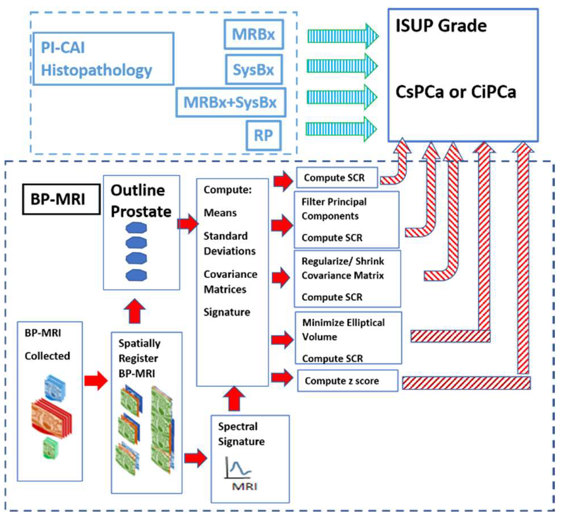
2.1. Overview
2.2. Study Design and Population
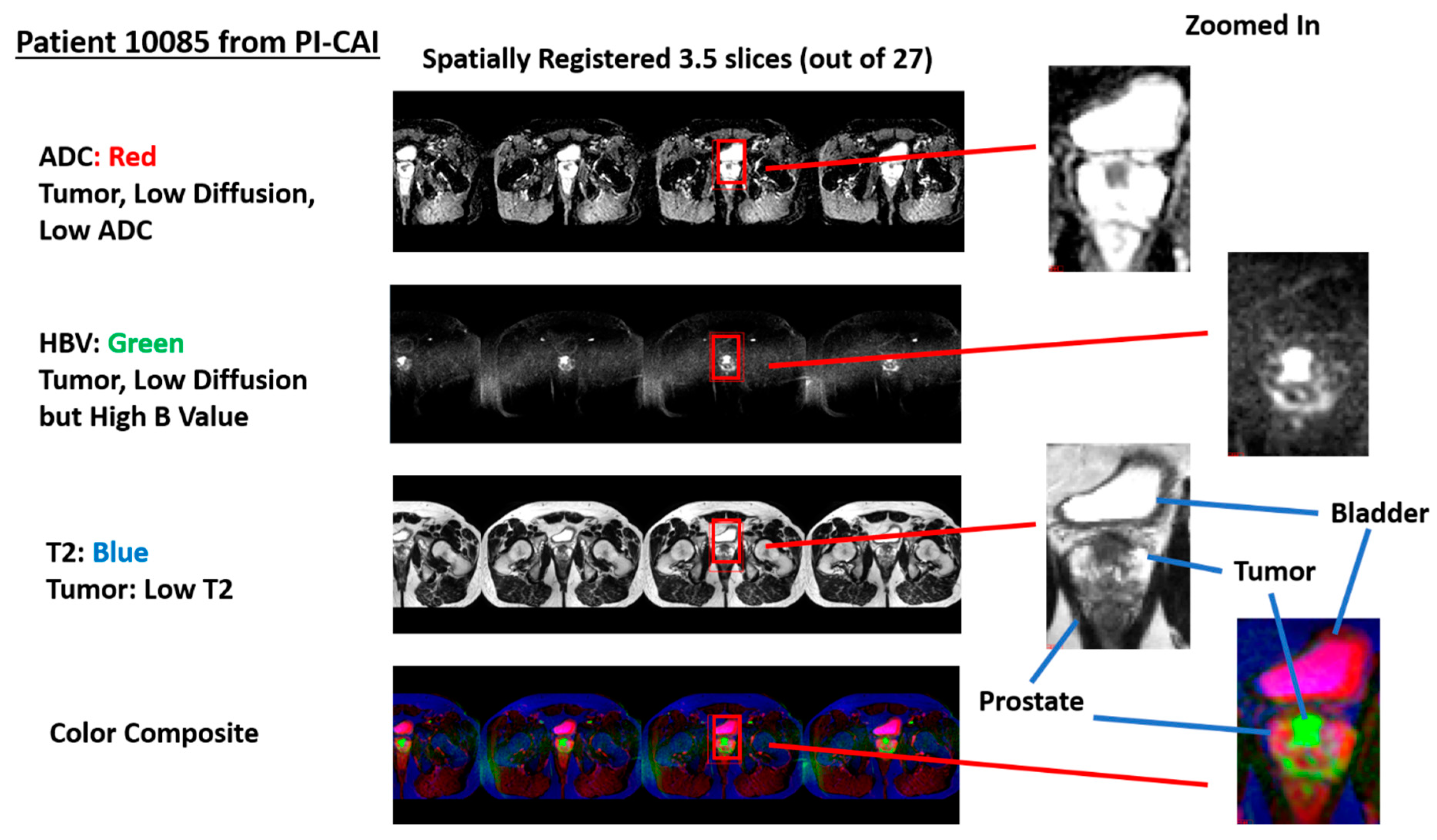
2.3. Spatial Registered Hypercube Assembly: Magnetic Resonance Imaging
2.4. Spatial Registered Hypercube Assembly: Image Processing, Pre-Analysis
2.5. Overall Quantitative Metrics Description: SCR, Z-Score
2.6. SCR: Filtering Noise
2.7. Regularization and Shrinkage
2.8. Elliptical Volume Minimization
2.9. Logistic Regression
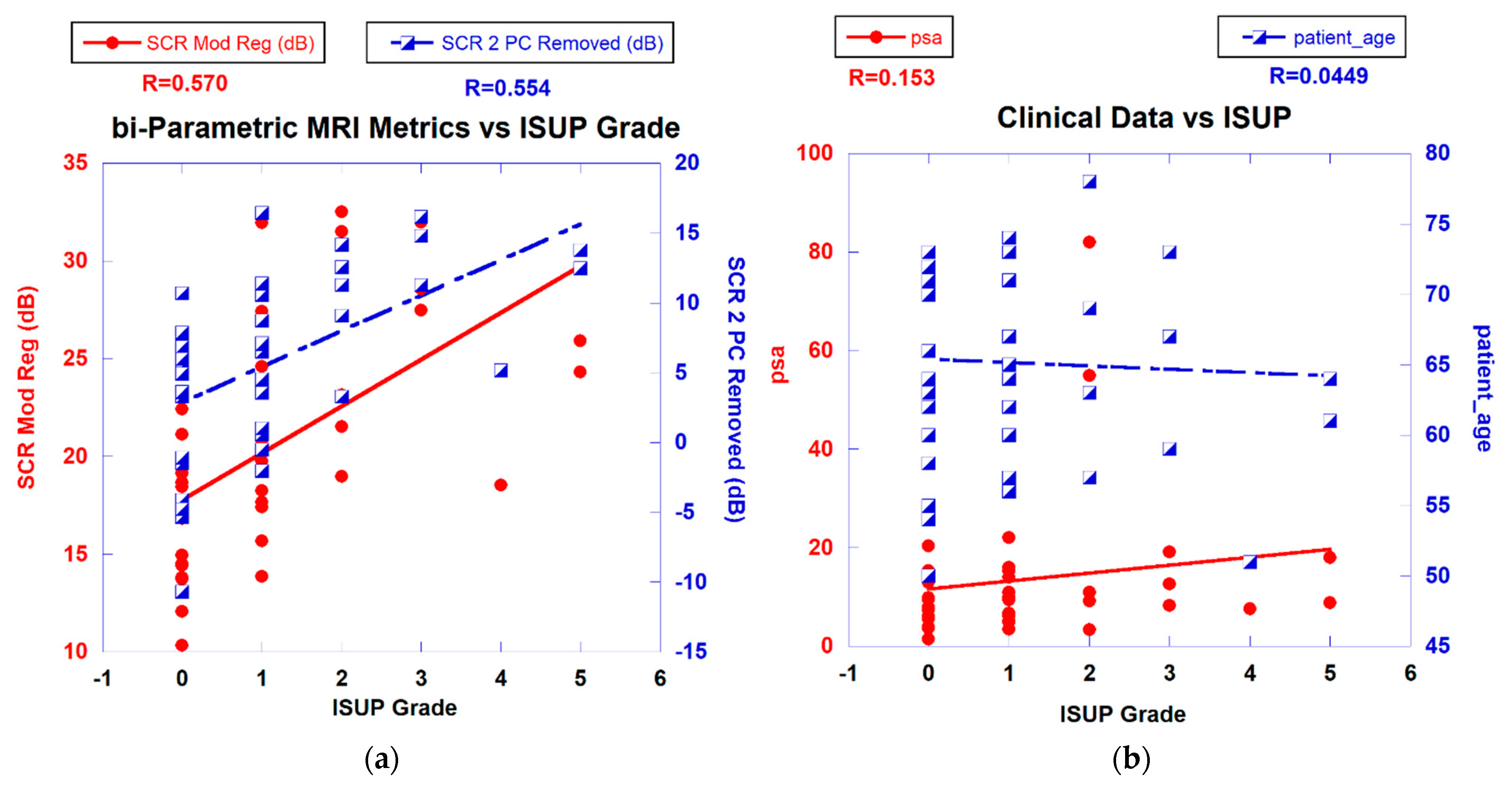
3. Results
4. Discussion
5. Conclusions
Author Contributions
Funding
Institutional Review Board Statement
Informed Consent Statement
Data Availability Statement
Conflicts of Interest
Appendix A
Appendix A.1. Overall Quantitative Metrics Description: SCR, Z-Score
Appendix A.2. SCR: Filtering Noise
Appendix A.3. Regularization and Shrinkage
References
- Sobin, L.; Wittekind, C. TNM Classification of Malignant Tumors, 5th ed.; John Wiley and Sons, Inc.: New York, NY, USA, 1997. [Google Scholar]
- Shariat, S.F.; Karakiewicz, P.I.; Roehrborn, C.G.; Kattan, M.W. An Updated Catalog of Prostate Cancer Predictive Tools. Cancer 2008, 113, 3075–3099. [Google Scholar] [CrossRef]
- Martin, N.E.; Mucci, L.A.; Loda, M.; DePinho, R. Prognostic Determinants in Prostate Cancer. Cancer J. 2011, 17, 429–437. [Google Scholar] [CrossRef]
- Parker, C.; Castro, E.; Fizazi, K.; Heidenreich, A.; Ost, P.; Procopio, G.; Tombal, B.; Gillessen, S. Prostate cancer: ESMO Clinical Practice Guidelines for diagnosis, treatment and follow-up. Ann. Oncol. 2020, 31, 1119–1134. [Google Scholar] [CrossRef]
- Bernal-Soriano, M.C.; Parker, L.A.; López-Garrigos, M.; Hernández-Aguado, I.; Caballero-Romeu, J.P.; Gómez-Pérez, L.; Alfayate-Guerra, R.; Pastor-Valero, M.; García, N.; Lumbreras, B. Factors associated with false negative and false positive results of prostate-specific antigen (PSA) and the impact on patient health: Cohort study protocol. Medicine 2019, 98, e17451. [Google Scholar] [CrossRef] [PubMed]
- Madej, A.; Wilkosz, J.; Różański, W.; Lipinski, M. Complication rates after prostate biopsy according to the number of sampled cores. Cent. Eur. J. Urol. 2012, 65, 116–118. [Google Scholar] [CrossRef]
- Bjurlin, M.A.; Meng, X.; Le Nobin, J.; Wysock, J.S.; Lepor, H.; Rosenkrantz, A.B.; Taneja, S.S. Optimization of prostate biopsy: The role of magnetic resonance imaging targeted biopsy in detection, localization and risk assessment. J. Urol. 2014, 192, 648–658. [Google Scholar] [CrossRef]
- Humphrey, P.A. Histopathology of Prostate Cancer. Cold Spring Harb. Perspect. Med. 2017, 7, a030411. [Google Scholar] [CrossRef]
- Turkbey, B.; Rosenkrantz, A.B.; Haider, M.A.; Padhani, A.R.; Villeirs, G.; Macura, K.J.; Tempany, C.M.; Choyke, P.L.; Cornud, F.; Margolis, D.J.; et al. PI-RADS Prostate Imaging-Reporting and Version 2.1: 2019 Update of Prostate Imaging Reporting and Data System Version 2. Eur. Urol. 2019, 76, 340–351. [Google Scholar] [CrossRef]
- Rosenkrantz, A.B.; Ginocchio, L.A.; Cornfeld, D.; Froemming, A.T.; Gupta, R.; Turkbey, B.; Westphalen, A.C.; Babb, J.S.; Margolis, D.J. Interobserver Reproducibility of the PI-RADS Version 2 Lexicon: A Multicenter Study of Six Experienced Prostate Radiologists. Radiology 2016, 280, 793–804. [Google Scholar] [CrossRef]
- Twilt, J.J.; van Leeuwen, K.G.; Huisman, H.J.; Fütterer, J.J.; de Rooij, M. Artificial Intelligence Based Algorithms for Prostate Cancer Classification and Detection on Magnetic Resonance Imaging: A Narrative Review. Diagnostics 2021, 11, 959. [Google Scholar] [CrossRef] [PubMed]
- Barragán-Montero, A.; Javaid, U.; Valdés, G.; Nguyen, D.; Desbordes, P.; Macq, B.; Willems, S.; Vandewinckele, L.; Holmström, M.; Löfman, F.; et al. Artificial intelligence and machine learning for medical imaging: A technology review. Phys. Med. 2021, 83, 242–256. [Google Scholar] [CrossRef]
- Stabile, A.; Giganti, F.; Rosenkrantz, A.B.; Taneja, S.S.; Villeirs, G.; Gill, I.S.; Allen, C.; Emberton, M.; Moore, C.M.; Kasivisvanathan, V. Multiparametric MRI for prostate cancer diagnosis: Current status and future directions. Nat. Rev. Urol. 2020, 17, 41–61. [Google Scholar] [CrossRef]
- Tofts, P.S.; Brix, G.; Buckley, D.L.; Evelhoch, J.L.; Henderson, E.; Knopp, M.V.; Larsson, H.B.; Lee, T.Y.; Mayr, N.A.; Parker, G.J.; et al. Estimating Kinetic Parameters from Dynamic Contrast-EnhancedT1-Weighted MRI of a Diffusable Tracer: Standardized Quantities and Symbols. J. Magn. Res. Imaging 1999, 10, 223–232. [Google Scholar] [CrossRef]
- Tofts, P.S. T1-Weighted DCE Imaging Concepts: Modelling, Acquisition and Analysis. Magnetom. Flash 2010, 3, 31–39. [Google Scholar]
- Padhani, A.R.; Schoots, I.; Villeirs, G. Contrast Medium or No Contrast Medium for Prostate Cancer Diagnosis. That Is the Question. J. Magn. Reson. Imaging. 2021, 53, 13–22. [Google Scholar] [CrossRef] [PubMed]
- Tamada, T.; Kido, A.; Yamamoto, A.; Takeuchi, M.; Miyaji, Y.; Moriya, T.; Sone, T. Comparison of Biparametric and Multiparametric MRI for Clinically Significant Prostate Cancer Detection with PI-RADS Version 2.1. J. Magn. Reason. Imaging 2021, 53, 283–291. [Google Scholar] [CrossRef]
- Mayer, R.; Simone, C.B., 2nd; Skinner, W.; Turkbey, B.; Choyke, P. Pilot study for supervised target detection applied to spatially registered multiparametric MRI in order to non-invasively score prostate cancer. Comput. Biol. Med. 2018, 94, 65–73. [Google Scholar] [CrossRef]
- Mayer, R.; Simone, C.B., 2nd; Turkbey, B.; Choyke, P. Development and testing quantitative metrics from multi-parametric magnetic resonance imaging that predict Gleason score for prostate tumors. Quant. Imaging Med. Surg. 2022, 12, 1859–1870. [Google Scholar] [CrossRef] [PubMed]
- Mayer, R.; Turkbey, B.; Choyke, P.; Simone, C.B., 2nd. Combining and Analyzing Novel Multi-parametric MRI Metrics for Predicting Gleason Score. Quant. Imaging Med. Surg. 2022, 12, 3844–3859. [Google Scholar] [CrossRef]
- Mayer, R.; Turkbey, B.; Choyke, P.; Simone, C.B., 2nd. Pilot Study for Generating and Assessing Nomograms and Decision Curves Analysis to Predict Clinically Significant Prostate Cancer Using Only Spatially Registered Multi-Parametric MRI. Front. Oncol. Sec. Genitourin. Oncol. 2023, 13, 1066498. [Google Scholar] [CrossRef] [PubMed]
- Egevad, L.; Delahunt, B.; Srigley, J.R.; Samaratunga, H. International Society of Urological Pathology (ISUP) grading of prostate cancer—An ISUP consensus on contemporary grading. APMIS 2016, 124, 433–435. [Google Scholar] [CrossRef]
- Saha, A.; Twilt, J.J.; Bosma, J.S.; Van Ginneken, B.; Yakar, D.; Elschot, M.; Veltman, J.; Fütterer, J.; de Rooij, M.; Huisman, H. Artificial Intelligence and Radiologists at Prostate Cancer Detection in MRI: The PI-CAI Challenge (Study Protocol). Available online: https://zenodo.org/record/6624726#.ZGvT2nbMKM9 (accessed on 28 April 2023).
- Ahdoot, M.; Wilbur, A.R.; Reese, S.E.; Lebastchi, A.H.; Mehralivand, S.; Gomella, P.T.; Bloom, J.; Gurram, S.; Siddiqui, M.; Pinsky, P.; et al. MRI-Targeted, Systematic, and Combined Biopsy for Prostate Cancer Diagnosis. N. Engl. J. Med. 2020, 382, 917–928. [Google Scholar] [CrossRef]
- Strang, G. Linear Algebra and Its Applications, 4th ed.; Thomson, Brooks/Cole: Belmont, CA, USA, 2006. [Google Scholar]
- Manolakis, D.; Shaw, G. Detection algorithms for hyperspectral imaging applications. IEEE Sign. Process. Mag. 2002, 19, 29–43. [Google Scholar] [CrossRef]
- Chen, G.; Qian, S. Denoising of Hyperspectral Imagery Using Principal Component Analysis and Wavelet Shrinkage. IEEE Trans. Geosci. Remote Sens. 2011, 49, 973–980. [Google Scholar] [CrossRef]
- Friedman, J.H. Regularized Discriminant Analysis. J. Am. Stat. Assoc. 1989, 84, 165–175. [Google Scholar] [CrossRef]
- Rousseeuw, P.J.; Van Driessen, K. A fast algorithm for the minimum covariance determinant estimator. Technometrics 1999, 41, 212–223. [Google Scholar] [CrossRef]
- Hosmer, D.W., Jr.; Lemeshow, S.; Sturdivant, R.X. Applied Logistic Regression, 2nd ed.; Wiley: Hoboken, NJ, USA, 2000; ISBN 978-0-471-35632-5. [Google Scholar]
- Fawcett, T. An Introduction to ROC Analysis. Pattern Recognit. Lett. 2006, 27, 861–874. [Google Scholar] [CrossRef]


| Age Median (years) | Age Minimum (years) | Age Maximum (years) |
| 65.14 | 50 | 78 |
| PSA Median (ng/mL) | PSA. Minimum (ng/mL) | PSA, Maximum (ng/mL) |
| 13.49 | 1.5 | 81.95 |
| Prostate Volume Median (cc) | Prostate Volume, Minimum(cc) | Prostate Volume, Maximum (cc) |
| 60.6 | 19 | 192 |
| ISUP Grade | Patient # | |
| 0 | 17 | |
| 1 | 14 | |
| 2 | 5 | |
| 3 | 3 | |
| 4 | 1 | |
| 5 | 2 | |
| Scanner | Patient # | |
| Skyra | 24 | |
| Ingenia | 12 | |
| Trio Tim | 1 | |
| Aera | 2 | |
| Prisma Fit | 3 | |
| Histopathology Technique | Patient # | |
| SysBx | 15 | |
| MRBx | 16 | |
| SysBX+MRBx | 8 | |
| RP | 3 |
| R (ALL) | R (Skyra) | R (Ingenia) | R (MRBx) | R (SysBx) | R (MRBx + SysBx) | |
|---|---|---|---|---|---|---|
| Independent Variable | ||||||
| SCR (unprocessed) | 0.143 | 0.152 | 0.079 | 0.487 | 0.279 | 0.586 |
| SCR (Regularized) | 0.588 | 0.671 | 0.595 | 0.371 | 0.686 | 0.819 |
| SCR (Modified Regularization) | 0.57 | 0.634 | 0.733 | 0.452 | 0.7 | 0.628 |
| SCR (1 PC removed) | 0.425 | 0.553 | 0.571 | 0.018 | 0.654 | 0.792 |
| SCR (2 PC removed) | 0.554 | 0.65 | 0.588 | 0.356 | 0.668 | 0.781 |
| SCR (Elliptical Minimization) | 0.524 | 0.593 | 0.705 | 0.521 | 0.629 | 0.536 |
| z score | 0.532 | 0.622 | 0.706 | 0.439 | 0.685 | 0.641 |
| DR; Average Difference+/−95%C.I. | 0 | 0.077+/−0.027 | 0.092+/−0.073 | 0.099+/−0.172 | 0.139+/−0.033 | 0.207+/−0.118 |
| Area Under Curve (AUC) | 2.5%–97.5% AUC C.I. | |
|---|---|---|
| Independent Variable | ||
| SCR (unprocessed) | 0.636 | 0.267–1.0 |
| SCR (Regularized) | 1 | 1.0–1.0 |
| SCR (Modified Regularization) | 1 | 1.0–1.0 |
| SCR (1 PC removed) | 1 | 1.0–1.0 |
| SCR (2 PC removed) | 1 | 1.0–1.0 |
| SCR (Elliptical Minimization) | 0.909 | 0.727–1.0 |
| z score | 1 | 1.0–1.0 |
| PSA | 0.409 | 0.00–0.909 |
| Prostate Volume | 0.455 | 0.167–0.767 |
| Patient Age | 0.545 | 0.250–0.818 |
| PSA+Prostate Volume+Patient Age | 0.5 | 0–1 |
| Prostate Volume+Patient Age | 0.455 | 0.167–0.767 |
Disclaimer/Publisher’s Note: The statements, opinions and data contained in all publications are solely those of the individual author(s) and contributor(s) and not of MDPI and/or the editor(s). MDPI and/or the editor(s) disclaim responsibility for any injury to people or property resulting from any ideas, methods, instructions or products referred to in the content. |
© 2023 by the authors. Licensee MDPI, Basel, Switzerland. This article is an open access article distributed under the terms and conditions of the Creative Commons Attribution (CC BY) license (https://creativecommons.org/licenses/by/4.0/).
Share and Cite
Mayer, R.; Turkbey, B.; Choyke, P.L.; Simone, C.B., II. Application of Spectral Algorithm Applied to Spatially Registered Bi-Parametric MRI to Predict Prostate Tumor Aggressiveness: A Pilot Study. Diagnostics 2023, 13, 2008. https://doi.org/10.3390/diagnostics13122008
Mayer R, Turkbey B, Choyke PL, Simone CB II. Application of Spectral Algorithm Applied to Spatially Registered Bi-Parametric MRI to Predict Prostate Tumor Aggressiveness: A Pilot Study. Diagnostics. 2023; 13(12):2008. https://doi.org/10.3390/diagnostics13122008
Chicago/Turabian StyleMayer, Rulon, Baris Turkbey, Peter L. Choyke, and Charles B. Simone, II. 2023. "Application of Spectral Algorithm Applied to Spatially Registered Bi-Parametric MRI to Predict Prostate Tumor Aggressiveness: A Pilot Study" Diagnostics 13, no. 12: 2008. https://doi.org/10.3390/diagnostics13122008
APA StyleMayer, R., Turkbey, B., Choyke, P. L., & Simone, C. B., II. (2023). Application of Spectral Algorithm Applied to Spatially Registered Bi-Parametric MRI to Predict Prostate Tumor Aggressiveness: A Pilot Study. Diagnostics, 13(12), 2008. https://doi.org/10.3390/diagnostics13122008