
HTLML: Hybrid AI Based Model for Detection of Alzheimer’s Disease

 ,
,  ,
,  ,
,
Abstract
:1. Introduction
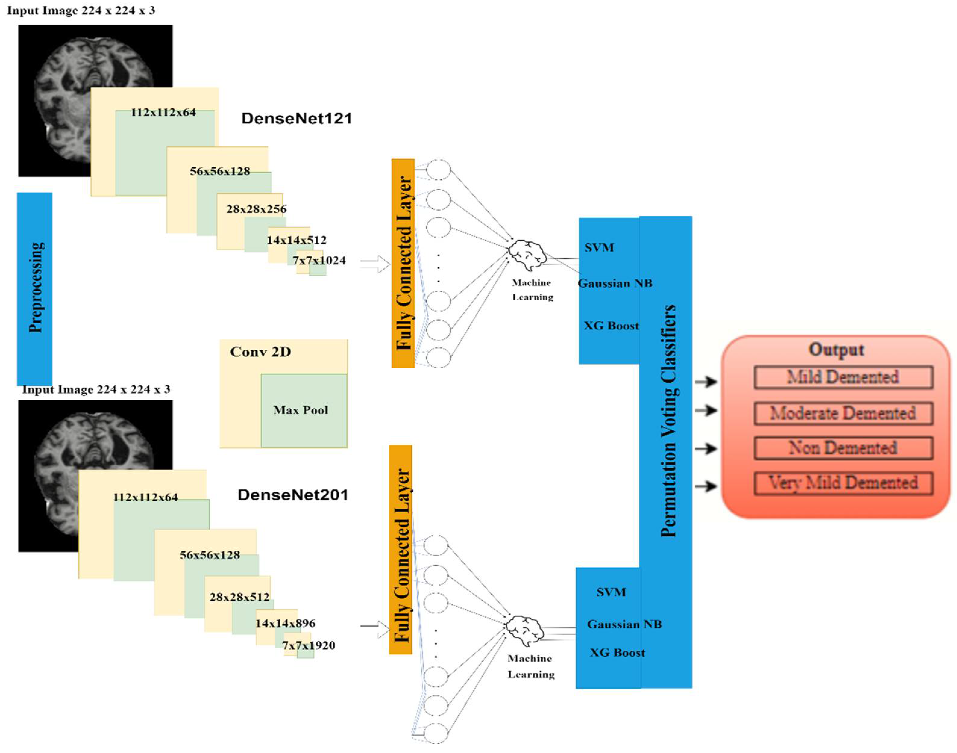
- A hybrid AI-based model was proposed by combining both transfer learning (TL) and permutation-based machine learning (ML) for AD diagnosis. The three hybrid DenseNet-121 models have been simulated with combinations of three machine learning classifiers, i.e., SVM, Gaussian naïve base and XGBoost, respectively, for detection of Alzheimer’s disease. From these models, the best hybrid DenseNet-121-SVM model was selected for further simulation.
- Two TL-based models were implemented, namely DenseNet-121 and DenseNet-201, for feature extraction.
- Finally, the three most popular machine learning (ML) classifiers, namely SVM, Gaussian naïve base and XGBoost, were respectively implemented for classification purposes.
- A permutation-based voting classifier was implemented for final accuracy observation.
- The proposed model was implemented using Adam optimizer and 1000 Epochs for evaluation purposes.
2. Background Literature
3. Proposed Research Methodology
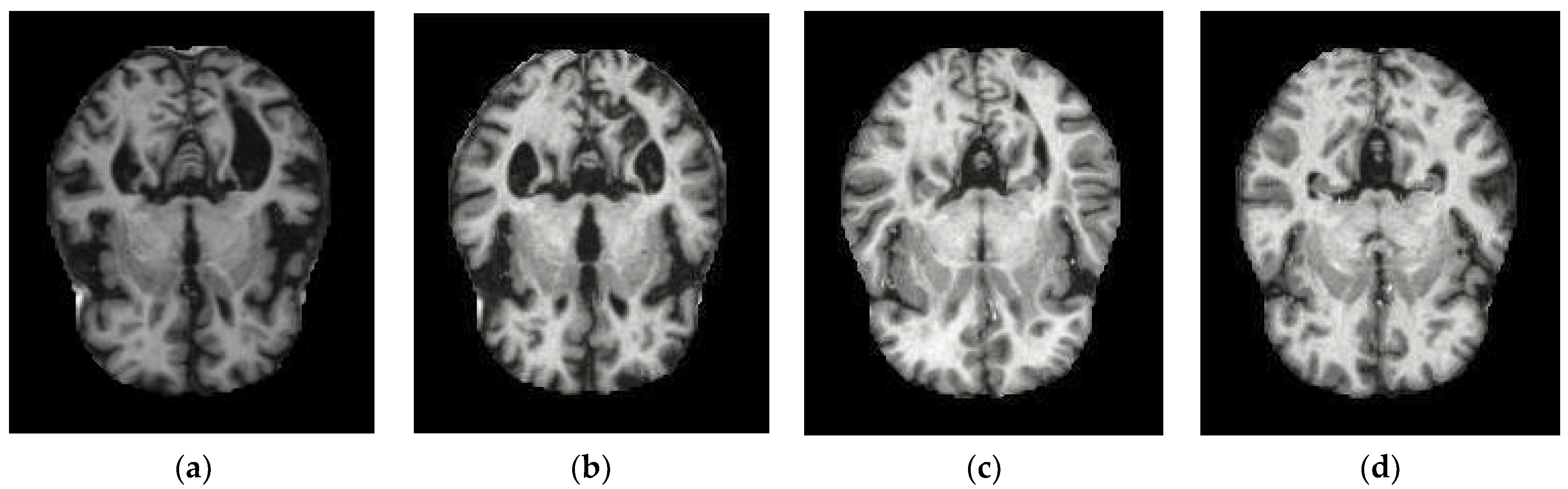
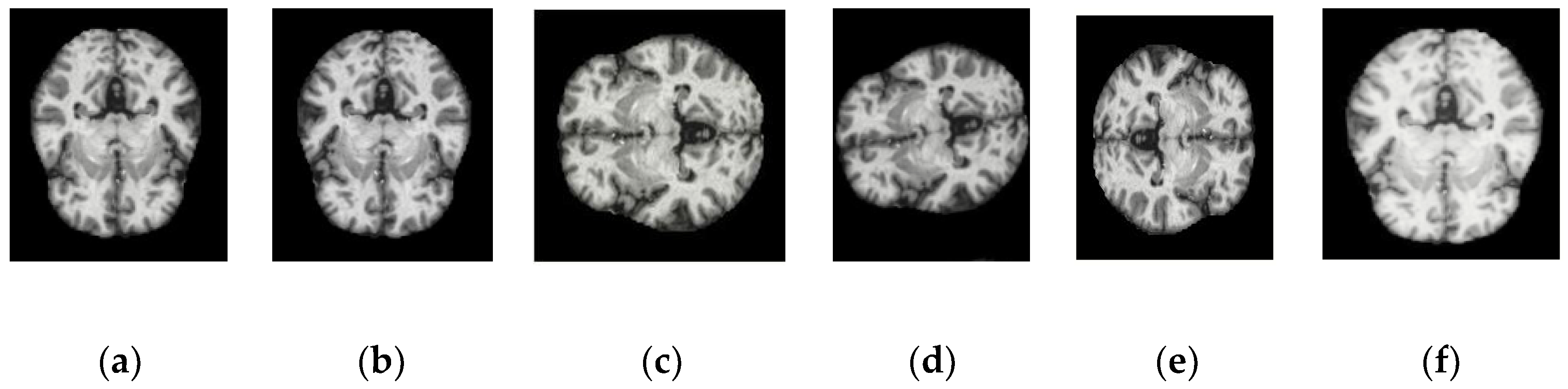
3.1. Input Dataset
3.2. Data Pre-Processing
3.2.1. Data Normalization
3.2.2. Data Augmentation
3.3. Feature Extraction Using Different DenseNet Transfer Learning Models
3.3.1. Feature Extraction Using DenseNet 121 Model
3.3.2. Feature Extraction Using DenseNet 201 Model
3.4. Classification Using Hybrid Machine Learning-Convolutional Neural Network
3.4.1. Gaussian Naïve Bayes Classifier
3.4.2. XGBoost Classifier
3.4.3. Support Vector Machine Classifier
4. Results Analysis
4.1. Analysis of Hybrid DenseNet 121 Model
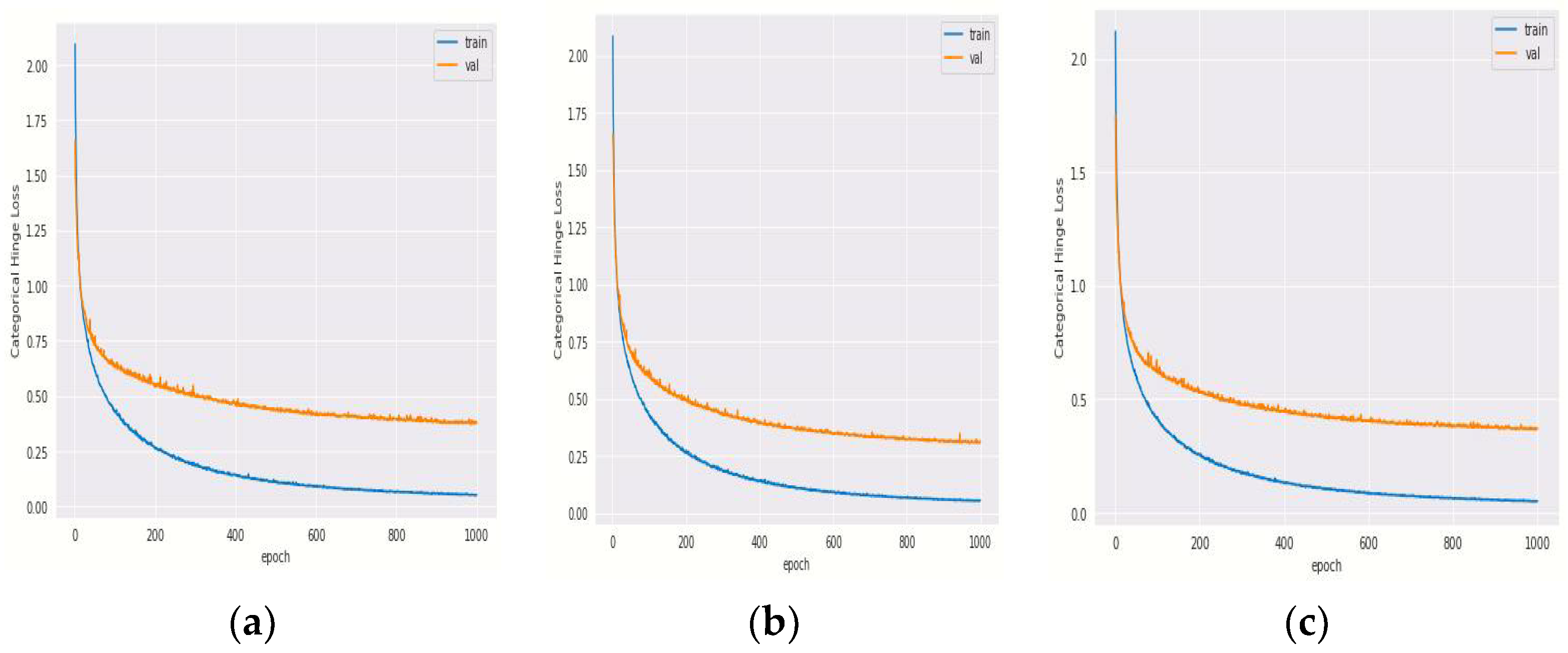
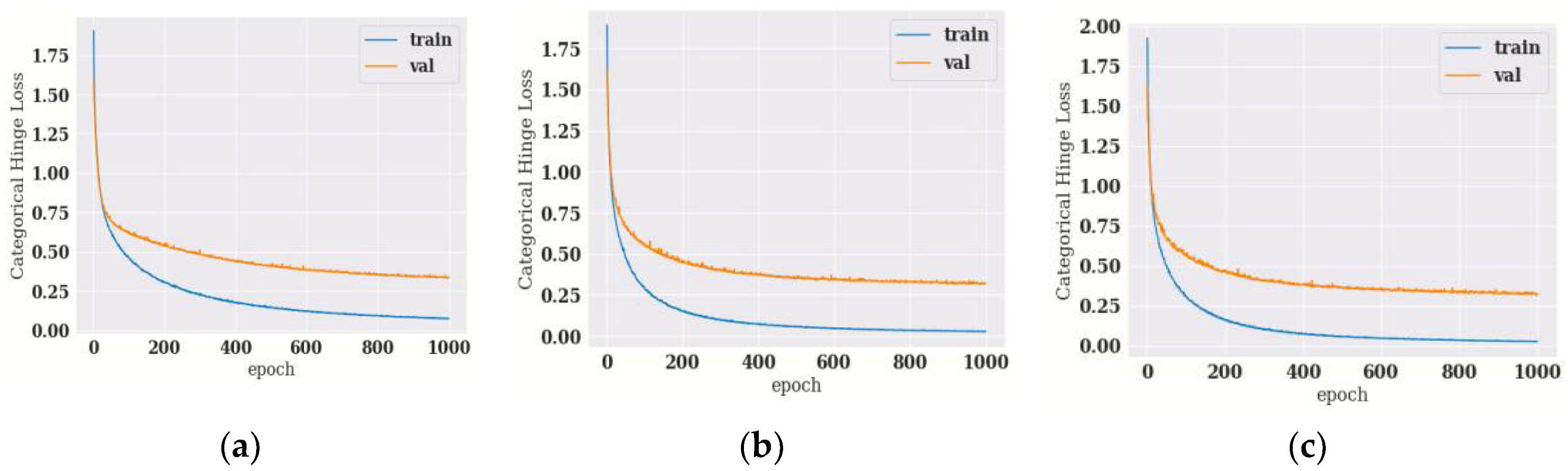
4.1.1. Training and Validation Loss of Hybrid DenseNet121 Models with Different Epochs
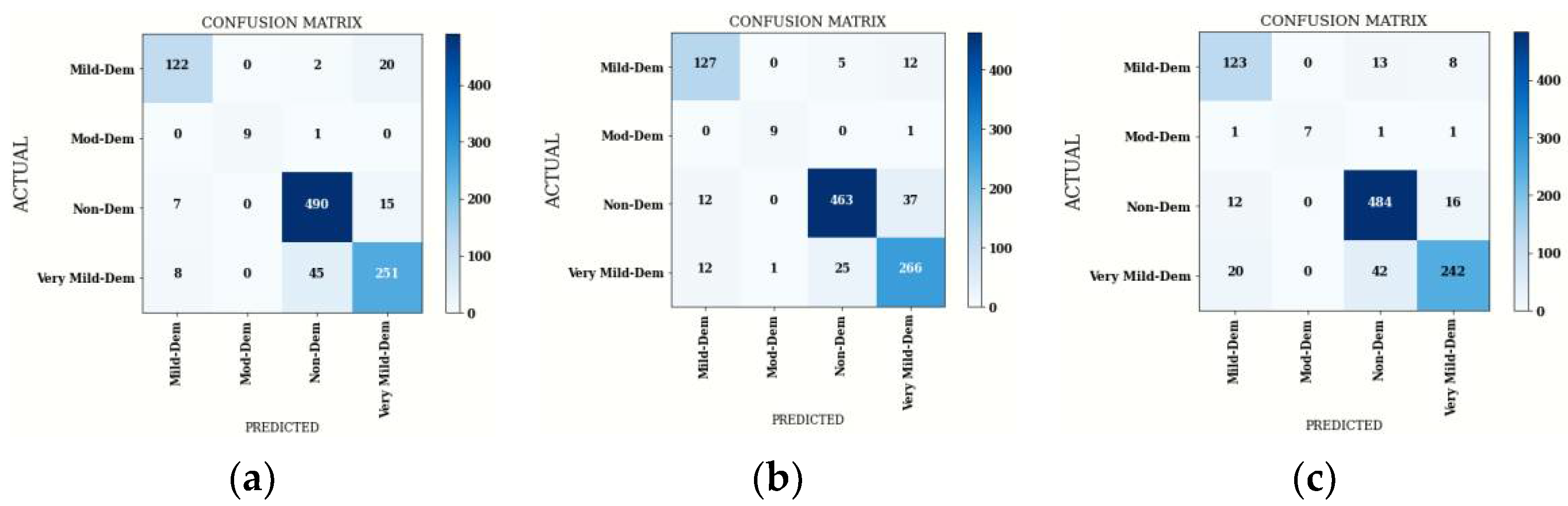
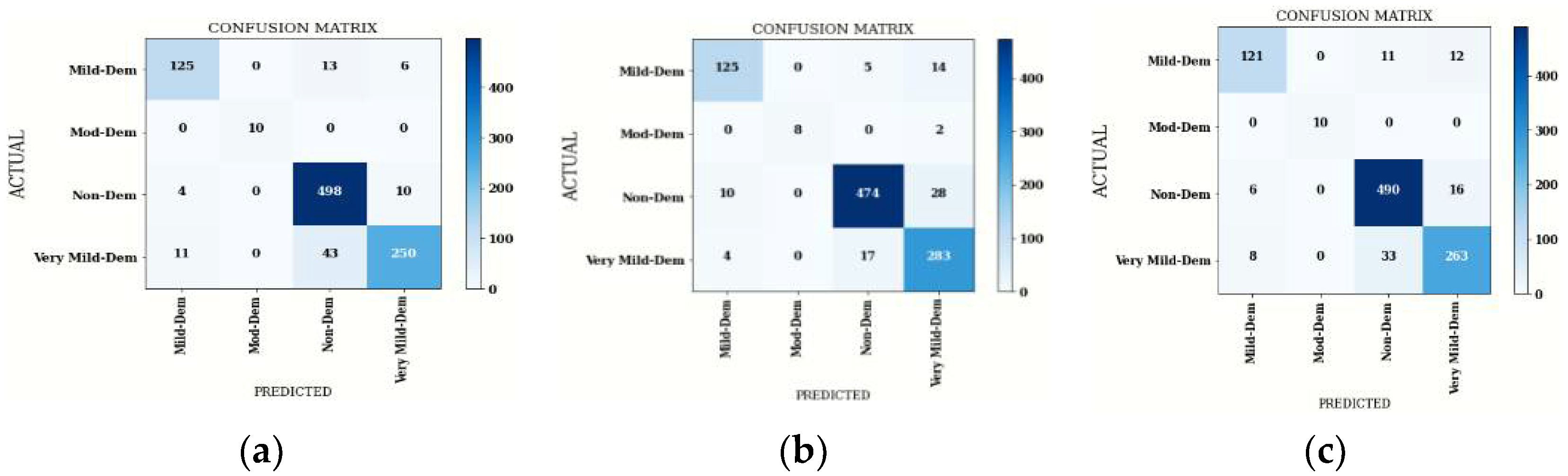
4.1.2. Confusion Matrix Comparison for Hybrid DenseNet121 Models
4.2. Analysis of Hybrid DenseNet 201 Model
4.2.1. Training and Validation Loss of Hybrid DenseNet201 Models with Different Epochs
4.2.2. Confusion Matrix Comparison for Hybrid DenseNet201 Model
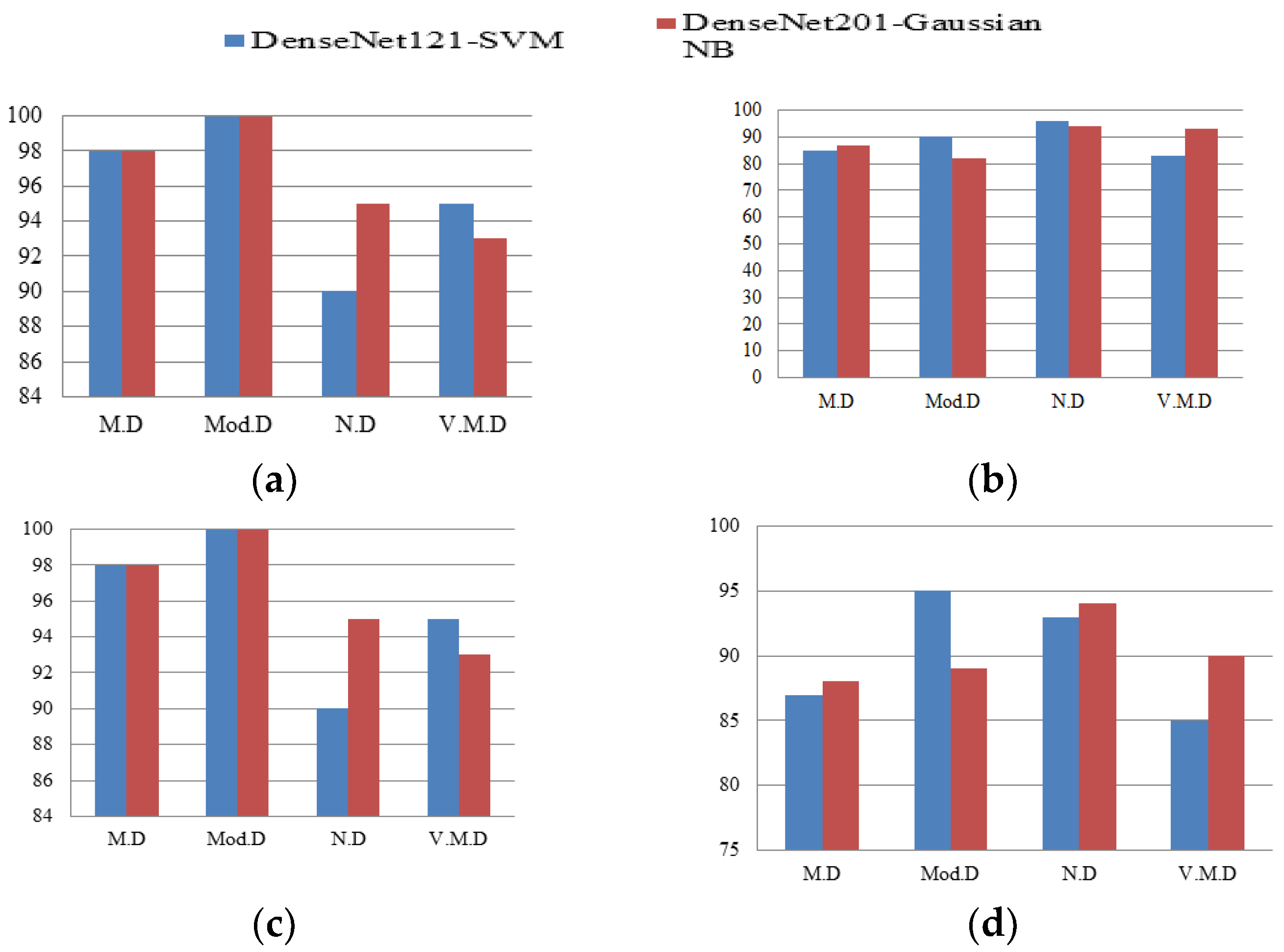
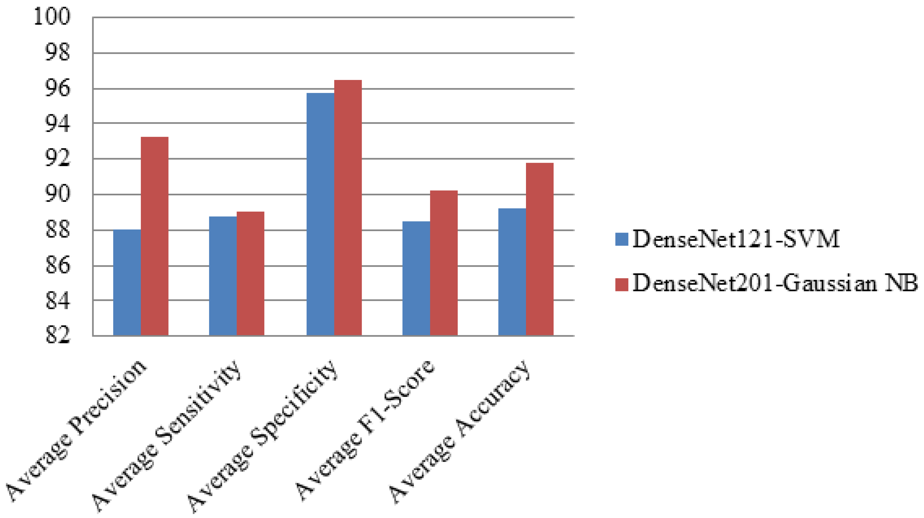
4.3. Comparison of Hybrid DenseNet121-SVM and DenseNet201-GNB Classifier
4.4. State of Art Comparison
5. Conclusions
Author Contributions
Funding
Institutional Review Board Statement
Informed Consent Statement
Data Availability Statement
Acknowledgments
Conflicts of Interest
References
- Krishna, I.; Murali, C.N.; Chakravarthy, A.S.N. A Hybrid Machine Learning Framework for Biomarkers Based ADNI Disease Prediction. Ilkogr. Online 2021, 20, 4902–4924. [Google Scholar]
- Feng, W.; Halm-Lutterodt, N.V.; Tang, H.; Mecum, A.; Mesregah, M.K.; Ma, Y.; Li, H.; Zhang, F.; Wu, Z.; Yao, E.; et al. Automated MRI-Based Deep Learning Model for Detection of Alzheimer’s Disease Process. IJNS 2020, 30, 2050032. [Google Scholar] [CrossRef] [PubMed]
- Ebrahimi-Ghahnavieh, A.; Luo, S.; Chiong, R. Transfer learning for Alzheimer’s disease detection on MRI images. IAICT 2019, 1, 133–138. [Google Scholar]
- Aderghal, K.; Khvostikov, A.; Krylov, A.; Benois-Pineau, J.; Afdel, K.; Catheline, G. Classification of Alzheimer disease on imaging modalities with deep CNNs using cross-modal transfer learning. CBMS 2018, 1, 345–350. [Google Scholar]
- Jha, D.; Kim, J.I.; Kwon, G.R. Diagnosis of Alzheimer’s disease using dual-tree complex wavelet transform, PCA, and feed-forward neural network. JHE 2017, 1, 100035. [Google Scholar] [CrossRef]
- Filipovych, R.; Davatzikos, C. Semi-supervised pattern classification of medical images: Application to mild cognitive impairment. NI 2011, 55, 1109–1119. [Google Scholar] [CrossRef] [PubMed] [Green Version]
- Rathore, S.; Habes, M.; Iftikhar, M.A.; Shacklett, A.; Davatzikos, C. A review on neuroimaging-based classification studies and associated feature extraction methods for Alzheimer’s disease and its prodromal stages. NI 2017, 155, 530–548. [Google Scholar] [CrossRef] [PubMed]
- Kang, W.; Lin, L.; Zhang, B.; Shen, X.; Wu, S. Multi-model and multi-slice ensemble learning architecture based on 2D convolutional neural networks for Alzheimer’s disease diagnosis. CBM 2021, 136, 104678. [Google Scholar] [CrossRef]
- Li, Y.; Fang, Y.; Wang, J.; Zhang, H.; Hu, B. Biomarker Extraction Based on Subspace Learning for the Prediction of Mild Cognitive Impairment Conversion. BMRI 2021, 1, 1940–1952. [Google Scholar] [CrossRef]
- Venugopalan, J.; Tong, L.; Hassanzadeh, H.R.; Wang, M.D. Multimodal deep learning models for early detection of Alzheimer’s disease stage. SR 2021, 11, 3254. [Google Scholar] [CrossRef]
- Nakagawa, T.; Ishida, M.; Naito, J.; Nagai, A.; Yamaguchi, S.; Onoda, K. Prediction of conversion to Alzheimer’s disease using deep survival analysis of MRI images. BC 2020, 2, fcaa057. [Google Scholar] [CrossRef] [PubMed]
- Talo, M.; Yildirim, O.; Baloglu, U.B.; Aydin, G.; Acharya, U.R. Convolutional neural networks for multi-class brain disease detection using MRI images. CMIG 2019, 78, 101673. [Google Scholar] [CrossRef] [PubMed]
- Acharya, U.R.; Fernandes, S.L.; WeiKoh, J.E.; Ciaccio, E.J.; Fabell, M.K.M.; Tanik, U.J.; Rajinikanth, V.; Yeong, C.H. Automated detection of Alzheimer’s disease using brain MRI images–A study with various feature extraction techniques. JMS 2019, 43, 302. [Google Scholar] [CrossRef] [PubMed]
- Islam, J.; Zhang, Y. Brain MRI analysis for Alzheimer’s disease diagnosis using an ensemble system of deep convolutional neural networks. BI 2018, 5, 2. [Google Scholar] [CrossRef] [PubMed]
- Hon, M.; Khan, N.M. Towards Alzheimer’s disease classification through transfer learning. In 2017 IEEE International conference on bioinformatics and biomedicine. BIBM 2017, 1, 1166–1169. [Google Scholar]
- Ali, E.M.; Seddik, A.F.; Haggag, M.H. Automatic detection and classification of Alzheimer’s disease from MRI using TANNN. IJCA 2016, 148, 283–294. [Google Scholar]
- Sarraf, S.; Tofighi, G. DeepAD: Alzheimer’s disease classification via deep convolutional neural networks using MRI and fMRI. BR 2016, 1, 070441. [Google Scholar]
- Zhao, Y.; Raichle, M.E.; Wen, J.; Benzinger, T.L.; Fagan, A.M.; Hassenstab, J.; Vlassenko, A.G.; Luo, J.; Cairns, N.J.; Christensen, J.J.; et al. In vivo detection of microstructural correlates of brain pathology in preclinical and early Alzheimer Disease with magnetic resonance imaging. NI 2017, 148, 296–304. [Google Scholar] [CrossRef] [Green Version]
- Fan, Y.; Resnick, S.M.; Wu, X.; Davatzikos, C. Structural and functional biomarkers of prodromal Alzheimer’s disease: A high-dimensional pattern classification study. NI 2008, 41, 277–285. [Google Scholar] [CrossRef] [Green Version]
- Misra, C.; Fan, Y.; Davatzikos, C. Baseline and longitudinal patterns of brain atrophy in MCI patients, and their use in prediction of short-term conversion to AD: Results from ADNI. NI 2009, 44, 1415–1422. [Google Scholar] [CrossRef] [Green Version]
- Moradi, E.; Pepe, A.; Gaser, C.; Huttunen, H.; Tohka, J. Machine learning framework for early MRI-based Alzheimer’s conversion prediction in MCI subjects. NI 2015, 104, 398–412. [Google Scholar] [CrossRef] [PubMed] [Green Version]
- Serra, L.; Cercignani, M.; Mastropasqua, C.; Torso, M.; Spanò, B.; Makovac, E.; Viola, V.; Giulietti, G.; Marra, C.; Caltagirone, C.; et al. Longitudinal changes in functional brain connectivity predicts conversion to Alzheimer’s disease. JAD 2016, 51, 377–389. [Google Scholar] [CrossRef] [PubMed]
- Fleming, A.; Bourdenx, M.; Fujimaki, M.; Karabiyik, C.; Krause, G.J.; Lopez, A.; Martín-Segura, A.; Puri, C.; Scrivo, A.; Skidmore, J.; et al. The different autophagy degradation pathways and neurodegeneration. Neuron 2022, 110, 935–966. [Google Scholar] [CrossRef] [PubMed]
- Yang, Y.; Arseni, D.; Zhang, W.; Huang, M.; Lövestam, S.; Schweighauser, M.; Kotecha, A.; Murzin, A.G.; Peak-Chew, S.Y.; Macdonald, J.; et al. Cryo-EM structures of amyloid-β 42 filaments from human brains. Science 2022, 375, 167–172. [Google Scholar] [CrossRef] [PubMed]
- Fang, E.F.; Hou, Y.; Palikaras, K.; Adriaanse, B.A.; Kerr, J.S.; Yang, B.; Lautrup, S.; Hasan-Olive, M.M.; Caponio, D.; Dan, X.; et al. Mitophagy inhibits amyloid-β and tau pathology and reverses cognitive deficits in models of Alzheimer’s disease. Nat. Neurosci. 2019, 22, 401–412. [Google Scholar] [CrossRef]
- Xie, C.; Zhuang, X.X.; Niu, Z.; Ai, R.; Lautrup, S.; Zheng, S.; Jiang, Y.; Han, R.; Gupta, T.S.; Cao, S.; et al. Amelioration of Alzheimer’s disease pathology by mitophagy inducers identified via machine learning and a cross-species workflow. Nat. Biomed. Eng. 2022, 6, 76–93. [Google Scholar] [CrossRef]


| Citation | Approach | Objective | Challenges of the Approach |
|---|---|---|---|
| [1] | Non Linear SVM with 2D CNN | To develop an automated technique to classify normal, early and late mild AD subjects. | Dataset consisted of 1167 MRI images. It was able to achieve 75% while performing Bin.c. |
| [2] | 2D CNN, 3D CNN 3D CNN-SVM | To distinguish AD and MCI individuals from normal individuals and to improve value based care of affected individuals in medical facilities. | Dataset contained 3127, 3T T1-weighted images. It performed tertiary classification and was able to an accuracy of 88.9%. It also aims to focus on reverting MCI individuals to normal individuals, predict AD progression and improve diagnosis of AD in future. |
| [3] | GoogleNet, AlexNet, VGGNet16VGGNet19SqueezeNetResNet18 ResNet50 ResNet101Inceptionv3. | To detect AD on MRI scans using D.L techniques. | Dataset consisted of 177 images. It performed Bin.c and achieved an accuracy of 84.38%. To include other neuro-imaging modalities such as PET scans or features in the system to take different aspects of AD into consideration. |
| [4] | Data Augmentation, CNN. | To classify AD by using Cross-Modal Transfer Learning | Dataset contained 416; sMRI image scans and it implemented Bin.c and achieved an accuracy of 83.57%. To proceed with a longitudinal dataset and develop a method based on spatial optimization of ROI. |
| [5] | DTCWT, PCA, FNN | To develop a CAD system to early diagnose AD individuals. | Dataset contained 416; T1- weighted image scans and it performed Bin.c and achieved an accuracy of 90.06%. Various feature reduction methods such as ICA, LDA and PCA were utilized for swarm optimization. |
| [6] | SVM, CNN | To classify AD from MCI by using semi-supervised SVM-CNN. | Dataset contained 359; T1- weighted images and it performed Bin.c and achieved an accuracy of 82.91%. To distinguish brain MRI images semi semi-supervised SVM is applied. |
| [7] | SVM-REF, CNN | To classify AD by using SVM-REF-CNN. | Dataset contained 1167; T1-weighted image scans and it performed Bin.c and achieved an accuracy of 81%. To distinguish brain images by using SVM-REF. |
| [8] | 2D-CNN, VGG16 | To classify AD by using ensemble based CNN. | Dataset contained 798; T1-weighted image scans and it performed Bin.c and achieved an accuracy of 90.36%. To distinguish AD from MCI images by using 2D-CNN. |
| [9] | SVM, CNN | To distinguish MCI from AD by using an SVM classifier with a linear kernel. | Dataset contained 1167; T1-weighted image scans and it performed Bin.c and achieved an accuracy of 69.37%. To distinguish AD from MCI images by using SVM-CNN. |
| [10] | SVM, k-NN, CNN | To distinguish MCI from AD by using SVM and k-NN. | Dataset contained 1311; T1 & T2 weighted image scans and it performed Bin.c and achieved an accuracy of 75%. To distinguish AD from MCI images by using SVN-CNN, KNN. |
| Dataset Source | Class Name | Training Images | Validating Images | Total Images |
|---|---|---|---|---|
| Kaggle | M.D Mod.D V.M.D N.D | 717 52 2560 1518 | 179 12 640 448 | 896 64 3200 1966 |
| S.No. | Name of the Class | Number of Images before Augmentation | Images after Augmentation | |
|---|---|---|---|---|
| Training Images | Validating Images | |||
| 1 | M.D | 896 | 2150 | 538 |
| 2 | Mod.D | 64 | 512 | 128 |
| 3 | N.D | 3200 | 2800 | 700 |
| 4 | V.M.D | 1966 | 3145 | 787 |
| Block Name | Layer Name | Input Size | Output Size | Filter Size | Number of Filters | Number of Times Block Run |
|---|---|---|---|---|---|---|
| Conv_1 | Conv_1_1 | 224 × 224 | 112 × 112 | 7 × 7 | 64 | 1 |
| Conv_2 | Conv_2_1:Conv_2_6 | 112 × 112 | 56 × 56 | 1 × 1 | 128 | 6 |
| Conv_3 | Conv_3_1:Conv_3_12 | 56 × 56 | 28 × 28 | 1 × 1 | 256 | 12 |
| Conv_4 | Conv_4_1:Conv_4_48 | 28 × 28 | 14 × 14 | 1 × 1 | 512 | 48 |
| Conv_5 | Conv_5_1:Conv_5_32 | 14 × 14 | 7 × 7 | 1 × 1 | 1024 | 32 |
| Block Name | Layer Name | Input Size | Output Size | Filter Size | Number of Filters | Number of Times Block Run |
|---|---|---|---|---|---|---|
| Conv_1 | Conv_1_1 | 224 × 224 | 112 × 112 | 7 × 7 | 64 | 1 |
| Conv_2 | Conv_2_1:Conv_2_12 | 112 × 112 | 56 × 56 | 1 × 1 | 128 | 12 |
| Conv_3 | Conv_3_1:Conv_3_24 | 56 × 56 | 28 × 28 | 1 × 1 | 512 | 24 |
| Conv_4 | Conv_4_1:Conv_4_96 | 28 × 28 | 14 × 14 | 1 × 1 | 896 | 96 |
| Conv_5 | Conv_5_1:Conv_5_64 | 14 × 14 | 7 × 7 | 1 × 1 | 1920 | 64 |
| Name of Corresponding Block | Filter for First Convolution Layer | Image for First Convolution Layer | Filter for Last Convolution Layer | Image for Last Convolution Layer |
|---|---|---|---|---|
| Conv_1 |  |  |  |  |
| Conv_2 |  | 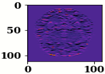 |  |  |
| Conv_3 |  | 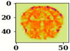 |  |  |
| Conv_4 |  |  |  | 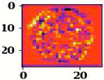 |
| Conv_5 |  | 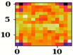 |  |  |
| Name of Block | Filter for First Convolution Layer | Image for First Convolution Layer | Filter for last Convolution Layer | Image for Last Convolution Layer |
|---|---|---|---|---|
| Conv_1 |  | 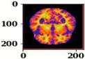 |  |  |
| Conv_2 |  | 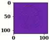 |  |  |
| Conv_3 |  |  |  |  |
| Conv_4 |  |  | 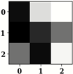 |  |
| Conv_5 |  |  | 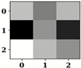 |  |
| Block Name | Layer Name | Input Size | Output Size | Filter Size | Number of Filters | Number of Times Block Run |
|---|---|---|---|---|---|---|
| Conv_5 | Conv_5_1:Conv_5_32 | 14 × 14 | 7 × 7 | 1 × 1 | 1024 | 32 |
| Conv_5 | Machine Learning Classifiers | 7 × 7 | 4 × 1 | 1 × 1 | 1024 | 32 |
| Dense_4 | Dense | 4 × 1 | 4 × 1 | N.A | N.A | 1 |
| Block Name | Layer Name | Input Size | Output Size | Filter Size | Number of Filters | Number of Times Block Run |
|---|---|---|---|---|---|---|
| Conv_5 | Conv_5_1:Conv_5_64 | 14 × 14 | 7 × 7 | 1 × 1 | 1920 | 64 |
| Conv_5 | Machine Learning Classifiers | 7 × 7 | 4 × 1 | 1 × 1 | 1920 | 64 |
| Dense_4 | Dense | 4 × 1 | 4 × 1 | N.A | N.A | 1 |
| SVM | GNB | XG | ||||
|---|---|---|---|---|---|---|
| Epoch | Train Loss | Valid Loss | Train Loss | Valid Loss | Train Loss | Valid Loss |
| 200 | 0.264 | 0.554 | 0.265 | 0.497 | 0.262 | 0.531 |
| 400 | 0.14 | 0.467 | 0.141 | 0.402 | 0.125 | 0.45 |
| 600 | 0.089 | 0.422 | 0.088 | 0.348 | 0.086 | 0.405 |
| 800 | 0.068 | 0.394 | 0.065 | 0.323 | 0.059 | 0.384 |
| 1000 | 0.051 | 0.313 | 0.051 | 0.38 | 0.05 | 0.372 |
| SVM | GNB | XG | ||||||||||
|---|---|---|---|---|---|---|---|---|---|---|---|---|
| Type | P | S | Sp | F1 | P | S | Sp | F1 | P | S | Sp | F1 |
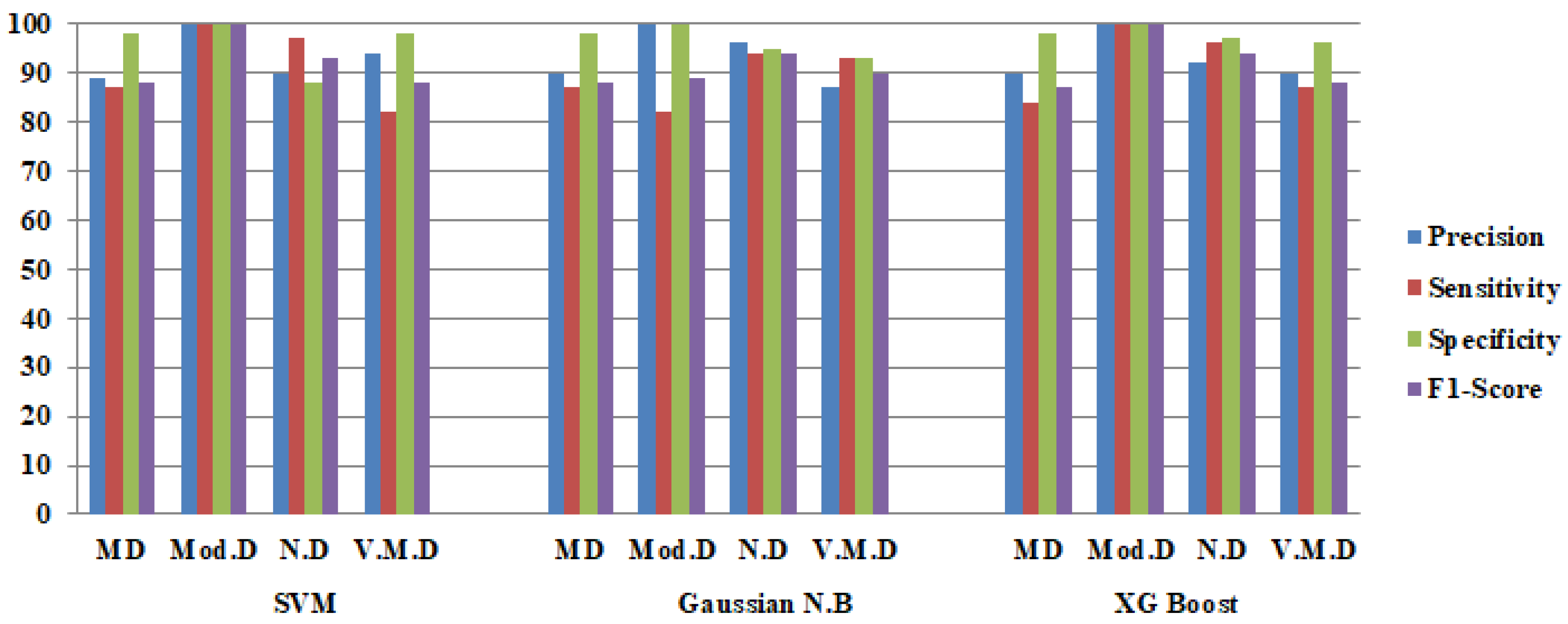
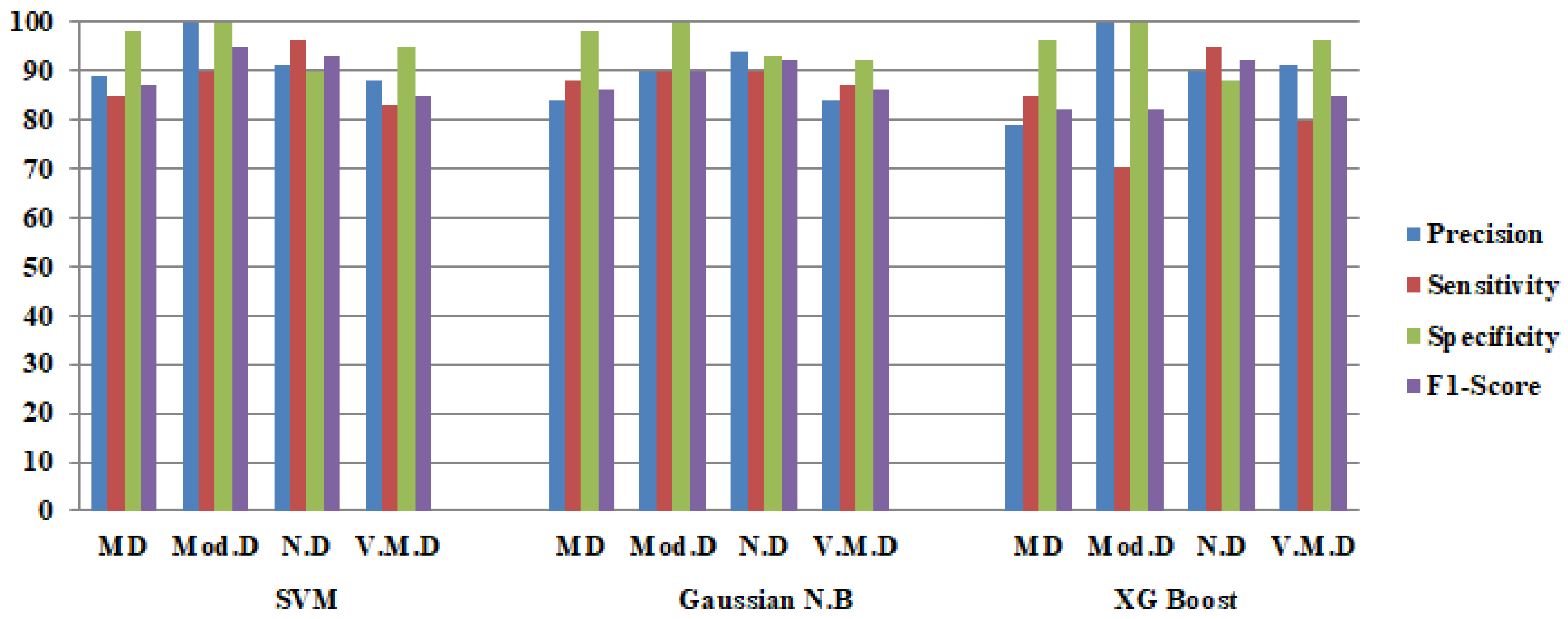
| Average | 92 | 89 | 96 | 90 | 88 | 89 | 96 | 89 | 90 | 83 | 95 | 85 |
| Accuracy | 89.89 | 89.18 | 88.25 | |||||||||
| SVM | GNB | XG | ||||
|---|---|---|---|---|---|---|
| Epoch | Train Loss | Valid Loss | Train Loss | Valid Loss | Train Loss | Valid Loss |
| 200 | 0.16 | 0.418 | 0.158 | 0.427 | 0.157 | 0.459 |
| 400 | 0.075 | 0.326 | 0.073 | 0.348 | 0.07 | 0.373 |
| 600 | 0.047 | 0.294 | 0.047 | 0.317 | 0.046 | 0.353 |
| 800 | 0.035 | 0.292 | 0.033 | 0.299 | 0.031 | 0.326 |
| 1000 | 0.027 | 0.291 | 0.028 | 0.265 | 0.025 | 0.318 |
| SVM | GNB | XG | ||||||||||
|---|---|---|---|---|---|---|---|---|---|---|---|---|
| Type | P | S | Sp | F | P | S | Sp | F | P | S | Sp | F |
| Average | 93 | 92 | 96 | 92 | 93 | 89 | 97 | 90 | 93 | 92 | 98 | 92 |
| Accuracy | 91.03 | 91.75 | 91.13 | |||||||||
| Study | Dataset Source | No. of Images | Technique Used | Accuracy |
|---|---|---|---|---|
| Rallabandi et al. [1] | ADNI | 1167 | SVM with D.L | 75% |
| Feng et al. [2] | ADNI | 3127 | 2D-CNN with D.L | 82.57% |
| Ebrahimi-Ghahnavieh et al. [3] | ADNI | 177 | DenseNet-201 ResNet50 | 84.38% 81.25% |
| Aderghal, K. et al. [4] | OASIS | 416 | Cross-Modal Transfer Learning | 83.57% |
| Jha et al. [5] | OASIS | 416 | DTCWT and PCA with FNN | 90.06% |
| Filipovych et al. [6] | ADNI | 359 | SVM, CNN | 82.91% |
| Rathore et al. [7] | ADNI | 1167 | SVM-REF, CNN | 81% |
| Kang et al. [8] | ADNI | 798 | 2D-CNN, VGG16 | 90.36% |
| Li et al. [9] | ADNI | 1167 | SVM, CNN | 69.37% |
| Venugopalan et al. [10] | ADNI | 1311 | SVM, k-NN, CNN | 75% |
| Proposed Methodology | Kaggle | 6400 | DenseNet201-Gaussian NB | 91.75% |
| DenseNet201-XG Boost | 91.13% | |||
| DenseNet201-SVM | 91.03% |
Publisher’s Note: MDPI stays neutral with regard to jurisdictional claims in published maps and institutional affiliations. |
© 2022 by the authors. Licensee MDPI, Basel, Switzerland. This article is an open access article distributed under the terms and conditions of the Creative Commons Attribution (CC BY) license (https://creativecommons.org/licenses/by/4.0/).
Share and Cite
Sharma, S.; Gupta, S.; Gupta, D.; Altameem, A.; Saudagar, A.K.J.; Poonia, R.C.; Nayak, S.R. HTLML: Hybrid AI Based Model for Detection of Alzheimer’s Disease. Diagnostics 2022, 12, 1833. https://doi.org/10.3390/diagnostics12081833
Sharma S, Gupta S, Gupta D, Altameem A, Saudagar AKJ, Poonia RC, Nayak SR. HTLML: Hybrid AI Based Model for Detection of Alzheimer’s Disease. Diagnostics. 2022; 12(8):1833. https://doi.org/10.3390/diagnostics12081833
Chicago/Turabian StyleSharma, Sarang, Sheifali Gupta, Deepali Gupta, Ayman Altameem, Abdul Khader Jilani Saudagar, Ramesh Chandra Poonia, and Soumya Ranjan Nayak. 2022. "HTLML: Hybrid AI Based Model for Detection of Alzheimer’s Disease" Diagnostics 12, no. 8: 1833. https://doi.org/10.3390/diagnostics12081833
APA StyleSharma, S., Gupta, S., Gupta, D., Altameem, A., Saudagar, A. K. J., Poonia, R. C., & Nayak, S. R. (2022). HTLML: Hybrid AI Based Model for Detection of Alzheimer’s Disease. Diagnostics, 12(8), 1833. https://doi.org/10.3390/diagnostics12081833