
Parkinson’s Disease Detection from Resting-State EEG Signals Using Common Spatial Pattern, Entropy, and Machine Learning Techniques


Abstract
:1. Introduction
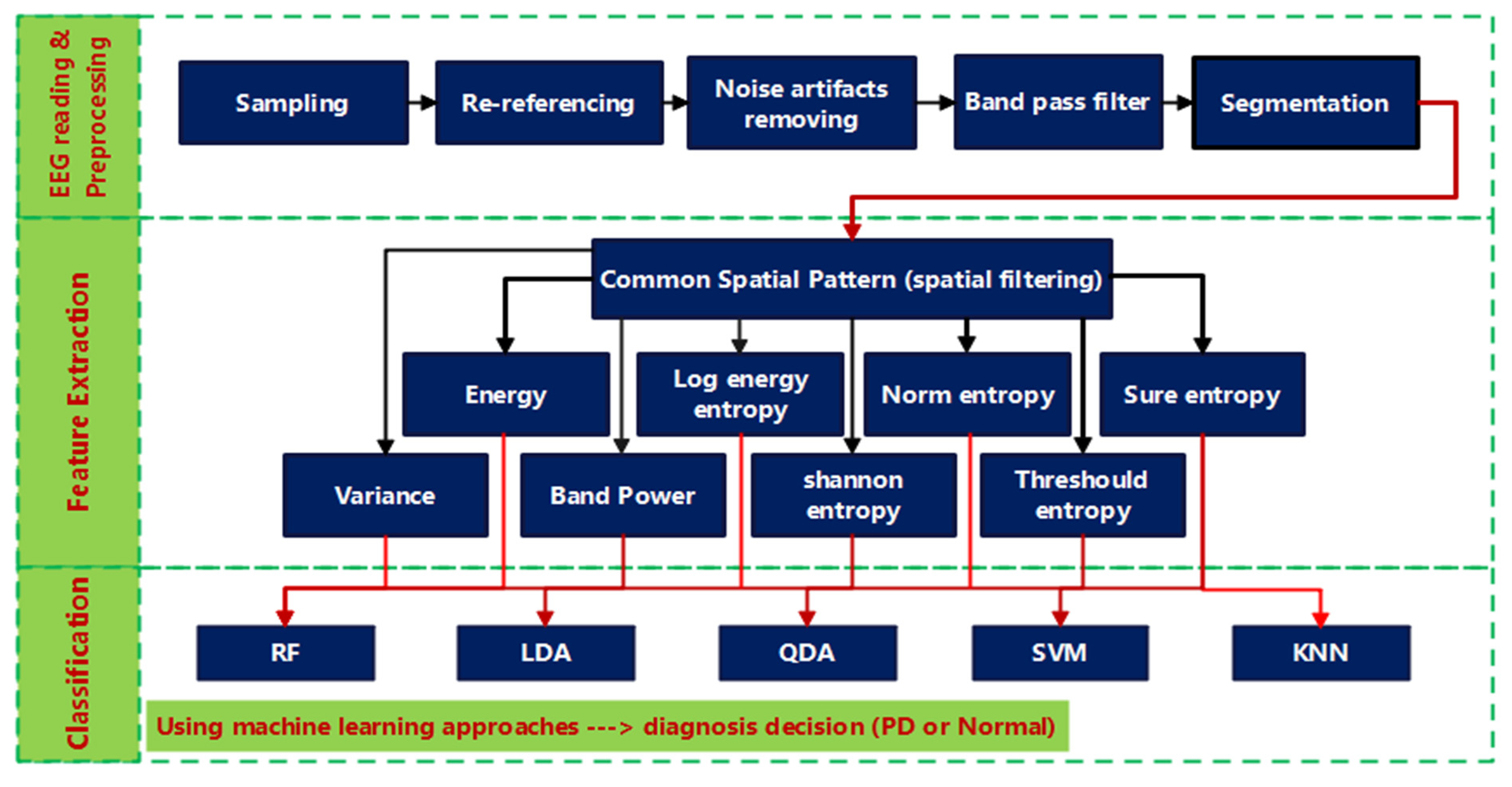
2. Methods
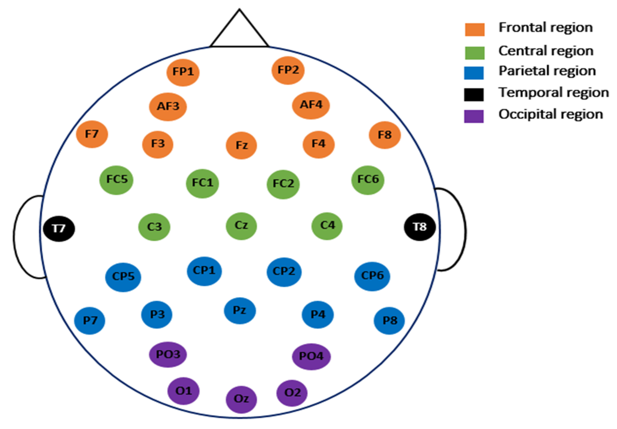
2.1. Data Description and Pre-Processing
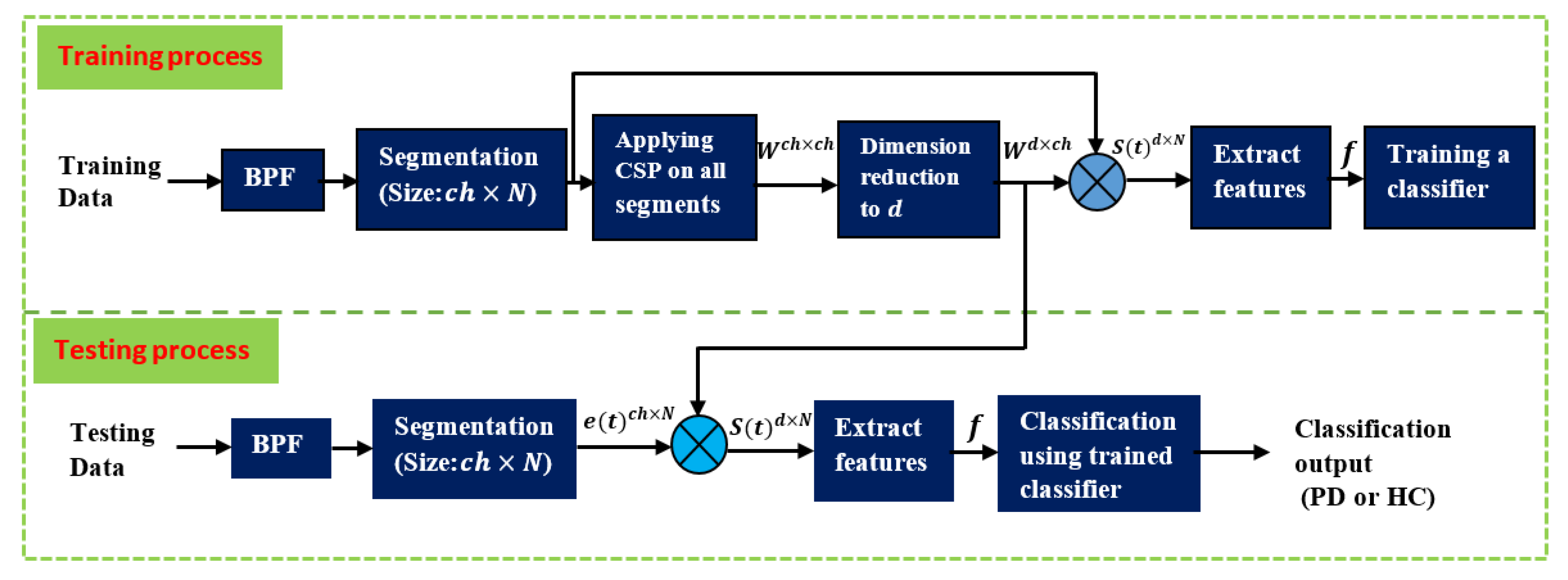
2.2. Common Spatial Pattern
2.3. Feature Extraction (FE)
- Energy (Eng) [40]
- Threshold entropy (ThEn) [44]where is the number of time instants for which the signal is greater than a threshold . The threshold is set to 0.2 based on trial-and-error to obtain the best accuracy.
- Norm entropy (NoEn) [44]where is the power of the entropy and must be such that 1 ≤ . In this study, it is selected to be 1.1.
- Sure entropy (SuEn) [44]where is the threshold value, and usually . In the present study, it is selected to be 3.
- Log energy entropy (LogEn) [44]
- Shannon entropy (ShEn) [44]
2.4. Classification and Problem Formulations
2.5. Performance Evaluation
3. Results and Discussion
3.1. SanDiego Dataset Results
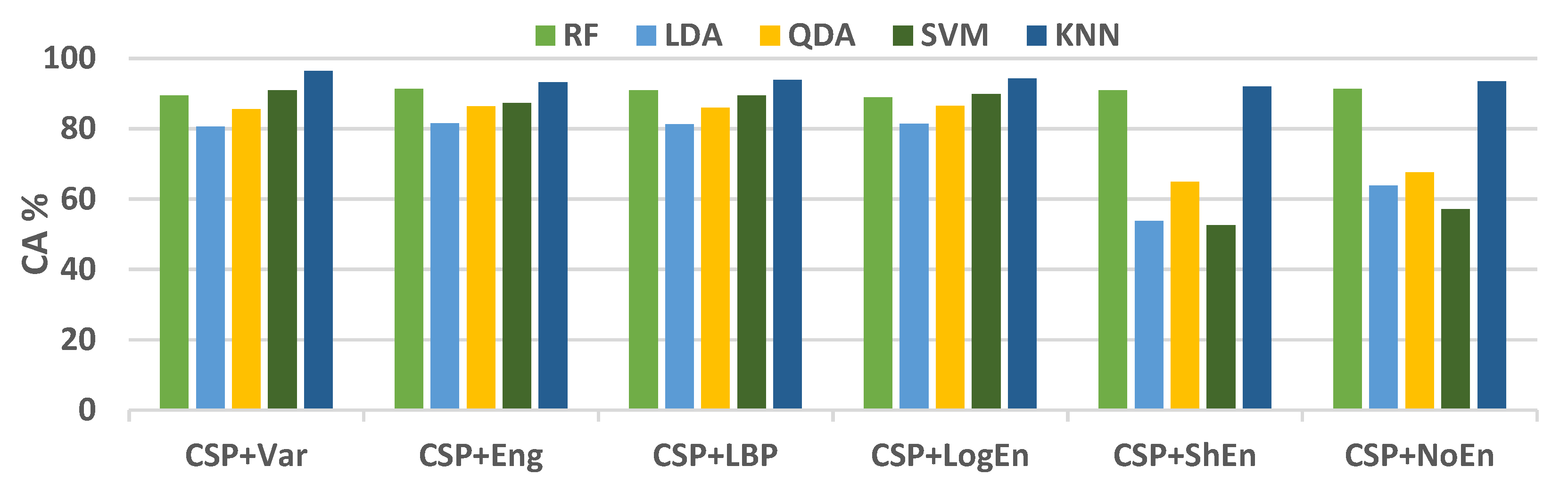
3.1.1. Off–Medication PD vs. Healthy Control
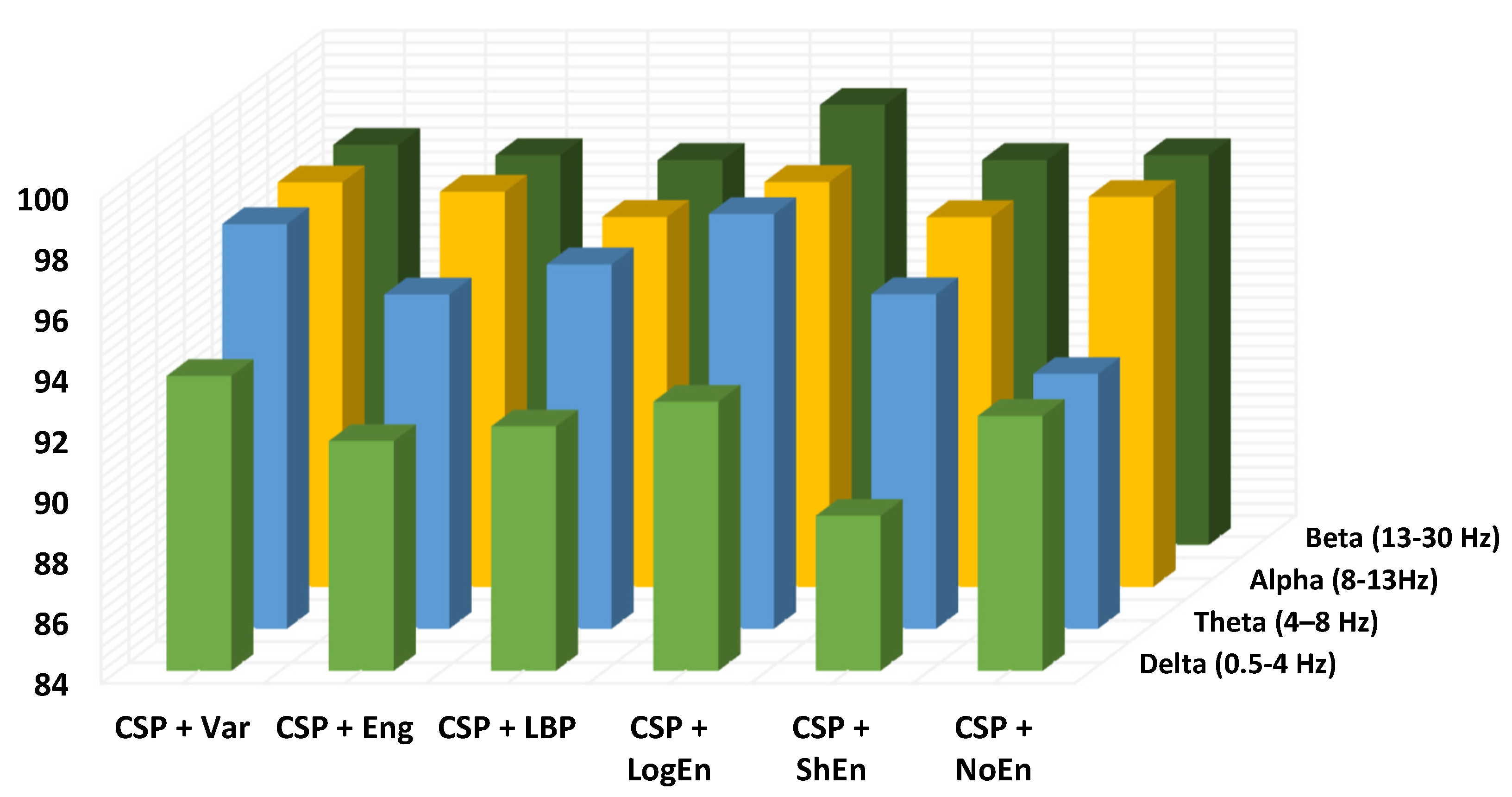
Investigation of Frequency Bands
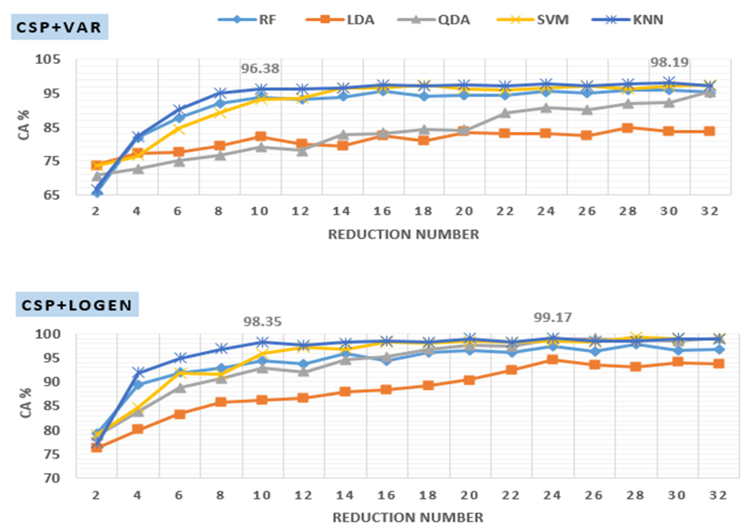
Investigation of Reduction Number
Investigation of Segment Length (SL)
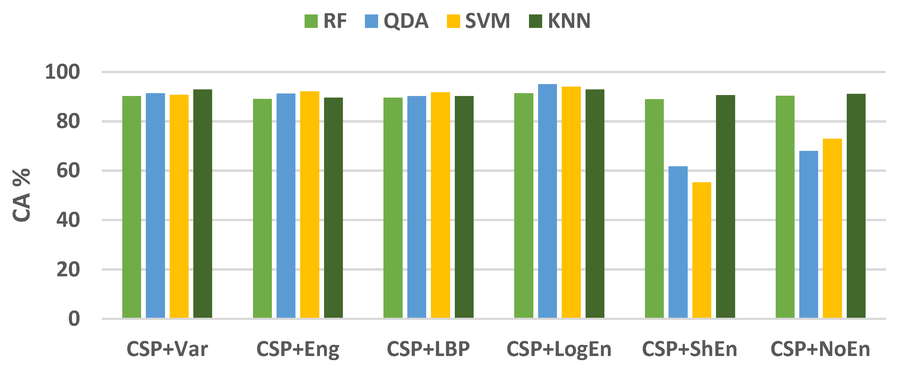
3.1.2. On–Medication PD vs. Health Control
3.1.3. Off–PD vs. On–PD
3.2. UNM-Based Results
- The proposed methods are simple and computationally efficient, making their hardware implementation easier and faster in reality.
- The proposed methods are robust as they have been developed using a ten-fold CV.
- The proposed methods achieved good classification accuracy as it has been validated using two datasets from two different sources.
- To the best of our knowledge, we are the first group to present CSP-based methods for the detection of PD.
4. Limitations and Future Studies
- Channel selection: In the present study, all the signals coming from all channels are used, and CSP is applied to spatially filter the signals and reduce the number of features by decreasing the value of . Selecting channels that contain only information important for the detection of Parkinson’s disease before applying signal processing was not exposed in this study. Future studies should be directed to using heuristic optimization methods to investigate the minimum number of channels that yield the maximum classification accuracy. PD detection using a few channels will be more practical and easier to use.
- Classification robustness: k-fold cross-validation is one of the most important techniques that are used to validate classification robustness. This technique was employed in all of the previous studies, shown in Table 16. In the present study, like in previous studies, k-fold cross-validation is also used to evaluate our proposed methods and compare their results with previous studies’ results. One of the disadvantages of this technique is that it may lead to the classification biasing problem resulting from data leakage. Therefore, future work includes the use of leave-one subject-out cross-validation along with k-fold.
- Source of data: One of the shortcomings of these types of studies is the use of different datasets, which makes the comparison of studies’ results unfair. It should specify a standard for evaluating the methods that are proposed by the researchers, including using public datasets. In the present study, two public datasets are used in order to compare the results of this study with those that used the same datasets. The authors also plan to test and confirm the proposed methods for additional brain disorders like autism and Alzheimer’s disease.
5. Conclusions
Author Contributions
Funding
Institutional Review Board Statement
Informed Consent Statement
Data Availability Statement
Conflicts of Interest
References
- National Institutes of Health (U.S.). Stem Cells: Scientific Progress and Future Research Directions; University Press of the Pacific: Honolulu, HI, USA, 2005.
- Poewe, W.; Seppi, K.; Tanner, C.; Halliday, G.M.; Brundin, P.; Volkmann, J.; Schrag, A.E.; Lang, A.E. Parkinson disease. Nat. Rev. Dis. Primers 2017, 3, 17013. [Google Scholar] [CrossRef] [PubMed]
- World Health Organization. Neurological Disorders: Public Health Challenges; WHO Press: Geneva, Switzerland, 2006; p. 177. [Google Scholar]
- Janca, A.; Aarli, J.A.; Prilipko, L.; Dua, T.; Saxena, S.; Saraceno, B. WHO/WFN Survey of neurological services: A worldwide perspective. J. Neurol. Sci. 2006, 247, 29–34. [Google Scholar] [CrossRef] [PubMed]
- Bhat, S.; Acharya, U.R.; Hagiwara, Y.; Dadmehr, N.; Adeli, H. Parkinson’s disease: Cause factors, measurable indicators, and early diagnosis. Comput. Biol. Med. 2018, 102, 234–241. [Google Scholar] [CrossRef] [PubMed]
- Parkinson’s Foundation. Available online: https://www.parkinson.org/understanding-parkinsons (accessed on 5 April 2022).
- Chaudhuri, K.R.; Healy, D.G.; Schapira, A.H.V. Non-motor symptoms of Parkinson’s disease: Diagnosis and management. Lancet Neurol. 2006, 5, 235–245. [Google Scholar] [CrossRef]
- Perlmutter, J.S. Assessment of Parkinson disease manifestations. Curr. Protoc. Neurosci. 2009, 49, 10.1.1–10.1.14. [Google Scholar] [CrossRef] [Green Version]
- ParkinsonsDisease.net. Parkinson’s Rating Scale. Available online: https://parkinsonsdisease.net/diagnosis/rating-scales-staging/ (accessed on 3 December 2021).
- Gómez-Vilda, P.; Mekyska, J.; Ferrández, J.M.; Palacios-Alonso, D.; Gómez-Rodellar, A.; Rodellar-Biarge, V.; Galaz, Z.; Smekal, Z.; Eliasova, I.; Kostalova, M.; et al. Parkinson disease detection from speech articulation neuromechanics. Front. Neuroinform. 2017, 11, 56. [Google Scholar] [CrossRef] [Green Version]
- Gupta, D.; Julka, A.; Jain, S.; Aggarwal, T.; Khanna, A.; Arunkumar, N.; Albuquerque, V.H.C. Optimized cuttlefish algorithm for diagnosis of Parkinson’s disease. Cogn. Syst. Res. 2018, 52, 36–48. [Google Scholar] [CrossRef]
- Jeancolas, L.; Benali, H.; Benkelfat, B.E.; Mangone, G.; Corvol, J.C.; Vidailhet, M.; Lehericy, S.; Petrovska-Delacrétaz, D. Automatic detection of early stages of Parkinson’s disease through acoustic voice analysis with mel-frequency Cepstral coefficients. In Proceedings of the 2017 International Conference on Advanced Technologies for Signal and Image Processing (ATSIP), Fez, Morocco, 22–24 May 2017; pp. 1–6. [Google Scholar]
- Joshi, D.; Khajuria, A.; Joshi, P. An automatic non-invasive method for Parkinson’s disease classification. Comput. Methods Programs Biomed. 2017, 145, 135–145. [Google Scholar] [CrossRef]
- Zeng, W.; Liu, F.; Wang, Q.; Wang, Y.; Ma, L.; Zhang, Y. Parkinson’s disease classification using gait analysis via deterministic learning. Neurosci. Lett. 2016, 633, 268–278. [Google Scholar] [CrossRef]
- Afonso, L.C.S.; Rosa, G.H.; Pereira, C.R.; Weber, S.A.; Hook, C.; Albuquerque, V.H.C.; Papa, J.P. A recurrence plot-based approach for Parkinson’s disease identification. Future Gener. Comput. Syst. 2019, 94, 282–292. [Google Scholar] [CrossRef]
- Rios-Urrego, C.D.; Vásquez-Correa, J.C.; Vargas-Bonilla, J.F.; Nöth, E.; Lopera, F.; Orozco-Arroyave, J.R. Analysis and evaluation of handwriting in patients with Parkinson’s disease using kinematic, geometrical, and non-linear features. Comput. Methods Programs Biomed. 2019, 173, 43–52. [Google Scholar] [CrossRef] [PubMed] [Green Version]
- Cigdem, O.; Beheshti, I.; Demirel, H. Effects of different covariates and contrasts on classification of Parkinson’s disease using structural MRI. Comput. Biol. Med. 2018, 99, 173–181. [Google Scholar] [CrossRef] [PubMed]
- Alturki, F.A.; AlSharabi, K.; Aljalal, M.; Abdurraqeeb, A.M. A DWT-Band power-SVM Based Architecture for Neurological Brain Disorders Diagnosis Using EEG Signals. In Proceedings of the 2019 2nd International Conference on Computer Applications & Information Security (ICCAIS), Riyadh, Saudi Arabia, 1–3 May 2019; pp. 1–4. [Google Scholar]
- Ibrahim, S.; Djemal, R.; Alsuwailem, A. Electroencephalography (EEG) signal processing for epilepsy and autism spectrum disorder diagnosis. Biocybern. Biomed. Eng. 2018, 38, 16–26. [Google Scholar] [CrossRef]
- Sheng, J.; Wang, B.; Zhang, Q.; Liu, Q.; Ma, Y.; Liu, W.; Shao, M.; Chen, B. A novel joint HCPMMP method for automatically classifying Alzheimer’s and deferent stage MCI patients. Behav. Brain Res. 2019, 365, 210–221. [Google Scholar] [CrossRef] [PubMed]
- Jahmunah, V.; Oh, S.L.; Rajinikanth, V.; Ciaccio, E.J.; Cheong, K.H.; Arunkumar, N.; Acharya, U.R. Automated detection of schizophrenia using nonlinear signal processing methods. Artif. Intell. Med. 2019, 100, 101698. [Google Scholar] [CrossRef] [PubMed]
- Chen, Y.; Gong, C.; Hao, H.; Guo, Y.; Xu, S.; Zhang, Y.; Yin, G.; Cao, X.; Yang, A.; Meng, F.; et al. Automatic Sleep Stage Classification Based on Subthalamic Local Field Potentials. IEEE Trans. Neural Syst. Rehabil. Eng. 2019, 27, 118–128. [Google Scholar] [CrossRef] [PubMed]
- Alturki, F.A.; AlSharabi, K.; Abdurraqeeb, A.M.; Aljalal, M. EEG Signal Analysis for Diagnosing Neurological Disorders Using Discrete Wavelet Transform and Intelligent Techniques. Sensors 2020, 20, 2505. [Google Scholar] [CrossRef]
- Ly, Q.T.; Handojoseno, A.A.; Gilat, M.; Chai, R.; Martens, K.A.E.; Georgiades, M.; Naik, G.R.; Tran, Y.; Lewis, S.J.; Nguyen, H.T. Detection of turning freeze in Parkinson’s disease based on S-transform decomposition of EEG signals. In Proceedings of the 2017 39th Annual International Conference of the IEEE Engineering in Medicine and Biology Society (EMBC), Jeju, Korea, 11–15 July 2017; pp. 3044–3047. [Google Scholar]
- Ly, Q.T.; Handojoseno, A.A.; Gilat, M.; Chai, R.; Martens, K.A.E.; Georgiades, M.; Naik, G.R.; Tran, Y.; Lewis, S.J.; Nguyen, H.T. Detection of gait initiation failure in Parkinson’s disease based on wavelet transform and support vector machine. In Proceedings of the 2017 39th Annual International Conference of the IEEE Engineering in Medicine and Biology Society (EMBC), Jeju, Korea, 11–15 July 2017; pp. 3048–3051. [Google Scholar]
- Ruffini, G.; Ibañez, D.; Castellano, M.; Dubreuil-Vall, L.; Soria-Frisch, A.; Postuma, R.; Gagnon, J.-F.; Montplaisir, J. Deep Learning with EEG Spectrograms in Rapid Eye Movement Behavior Disorder. Front. Neurol. 2019, 10, 806. [Google Scholar] [CrossRef] [Green Version]
- Chaturvedi, M.; Hatz, F.; Gschwandtner, U.; Bogaarts, J.G.; Meyer, A.; Fuhr, P.; Roth, V. Quantitative EEG (QEEG) measures differentiate Parkinson’s disease (PD) patients from healthy controls (HC). Front. Aging Neurosci. 2017, 9, 3. [Google Scholar] [CrossRef] [Green Version]
- Betrouni, N.; Delval, A.; Chaton, L.; Defebvre, L.; Duits, A.; Moonen, A.; Leentjens, A.F.G.; Dujardin, K. Electroencephalography-based machine learning for cognitive profiling in Parkinson’s disease: Preliminary results. Mov. Disord. 2019, 34, 210–217. [Google Scholar] [CrossRef]
- Yuvaraj, R.; Rajendra Acharya, U.; Hagiwara, Y. A novel Parkinson’s disease diagnosis index using higher-order spectra features in EEG signals. Neural Comput. Appl. 2018, 30, 1225–1235. [Google Scholar] [CrossRef]
- Oh, S.L.; Hagiwara, Y.; Raghavendra, U.; Yuvaraj, R.; Arunkumar, N.; Murugappan, M.; Acharya, U.R. A deep learning approach for Parkinson’s disease diagnosis from EEG signals. Neural Comput. Appl. 2020, 32, 10927–10933. [Google Scholar] [CrossRef]
- Shah, S.A.A.; Zhang, L.; Bais, A. Dynamical system based compact deep hybrid network for classification of Parkinson disease related EEG signals. Neural Netw. 2020, 130, 75–84. [Google Scholar] [CrossRef] [PubMed]
- Anjum, M.F.; Dasgupta, S.; Mudumbai, R.; Singh, A.; Cavanagh, G.F.; Narayanan, N.S. Linear predictive coding distinguishes spectral EEG features of Parkinson’s disease. Parkinsonism Relat. Disord. 2020, 79, 79–85. [Google Scholar] [CrossRef]
- Lee, S.; Hussein, R.; Ward, R.; Wang, Z.J.; McKeown, M.J. A convolutional-recurrent neural network approach to resting-state EEG classification in Parkinson’s disease. J. Neurosci. Methods 2021, 361, 109282. [Google Scholar] [CrossRef]
- Khare, S.K.; Bajaj, V.; Acharya, U.R. Detection of Parkinson’s disease using automated tunable Q wavelet tranform technique with EEG signals. Biocybern. Biomed. Eng. 2021, 41, 679–689. [Google Scholar] [CrossRef]
- Alturki, F.A.; Aljalal, M.; Abdurraqeeb, A.M.; Alsharabi, K.; Al-Shamma’A, A.A. Common Spatial Pattern Technique with EEG Signals for Diagnosis of Autism and Epilepsy Disorders. IEEE Access 2021, 9, 24334–24349. [Google Scholar] [CrossRef]
- Rockhill, A.P.; Jackson, N.; George, J.; Aron, A.; Swann, N.C. UC San Diego Resting State EEG Data from Patients with Parkinson’s Disease. OpenNeuro 2020. [Google Scholar] [CrossRef]
- George, J.S.; Strunk, J.; Mak-McCully, R.; Houser, M.; Poizner, H.; Aron, A.R. Dopaminergic therapy in Parkinson’s disease decreases cortical beta band coherence in the resting state and increases cortical beta band power during executive control. Neuroimage Clin. 2013, 3, 261–270. [Google Scholar] [CrossRef] [Green Version]
- Cavanagh, J.F.; Kumar, P.; Mueller, A.A.; Richardson, S.P.; Mueen, A. Diminished eeg habituation to novel events effectively classifies parkinson’s patients. Clin. Neurophysiol. 2018, 129, 409–418. [Google Scholar] [CrossRef]
- Blankertz, B.; Tomioka, R.; Lemm, S.; Kawanabe, M.; Muller, K.-R. Optimizing spatial filters for robust EEG single-trial analysis. IEEE Signal Process. Mag. 2007, 25, 41–56. [Google Scholar] [CrossRef]
- Hayes, M.H. Statistical Digital Signal Processing and Modeling; John Wiley & Sons: New York, NY, USA, 1996. [Google Scholar]
- Kannathal, N.; Choo, M.L.; Acharya, U.R.; Sadasivan, P.K. Entropies for detection of epilepsy in EEG. Comput. Methods Programs Biomed. 2005, 80, 187–194. [Google Scholar] [CrossRef] [PubMed]
- Joy, R.C.; George, S.T.; Rajan, A.A.; Subathra, M.S.P. Detection of ADHD from EEG Signals Using Different Entropy Measures and ANN. Clin. EEG Neurosci. 2022, 53, 12–23. [Google Scholar] [CrossRef]
- Bosl, W.; Tierney, A.; Tager-Flusberg, H.; Nelson, C. EEG complexity as a biomarker for autism spectrum disorder risk. BMC Med. 2011, 9, 18. [Google Scholar] [CrossRef] [Green Version]
- Coifman, R.R.; Wickerhauser, M.V. Entropy-based algorithms for best basis selection. IEEE Trans. Inf. Theory 1992, 38, 713–718. [Google Scholar] [CrossRef] [Green Version]
- Breiman, L. Random Forests. Mach. Learn. 2001, 45, 5–32. [Google Scholar] [CrossRef] [Green Version]
- Duda, R.O.; Hart, P.E. Pattern Classification; John Wiley & Sons: Hoboken, NJ, USA, 2012. [Google Scholar]
- Burges, C.J.C. A tutorial on support vector machines for pattern recognition. Data Min. Knowl. Discov. 1998, 2, 121–167. [Google Scholar] [CrossRef]
- Weinberger, K.Q.; Saul, L.K. Distance metric learning for large margin nearest neighbor classification. J. Mach. Learn. Res. 2009, 10, 207–244. [Google Scholar]
- Swift, A.; Heale, R.; Twycross, A. What are sensitivity and specificity? Evid.-Based Nurs. 2020, 23, 2–4. [Google Scholar] [CrossRef] [Green Version]
- Fawcett, T. An introduction to ROC analysis. Pattern Recognit. Lett. 2006, 27, 861–874. [Google Scholar] [CrossRef]
- Refaeilzadeh, P.; Tang, L.; Liu, H. Cross-validation. In Encyclopedia of Database System; Springer: Berlin/Heidelberg, Germany, 2009; pp. 532–538. [Google Scholar]


| Reference | FE Methods | Classifier(s) | Dataset | Classification Accuracy (%) |
|---|---|---|---|---|
| [29], 2018 | Higher-order spectra (HOS) | DT, KNN, FKNN, NB, PNN, SVM | Malaysian dataset | 90.6–99.6 |
| [30], 2020 | ---- | 13 layer CNN | Malaysian dataset | 88.25 |
| [31], 2020 | ---- | CNN+LSTM | UNM dataset | 99.2 |
| [32], 2020 | PSD | Hyperplanes | UNM dataset | 85.4 |
| [33], 2021 | -- | CNN+RNN | Own dataset | 99.2 |
| [34], 2021 | WT+statistical measures | SVM | SanDiego dataset | 96.13 |
| Dataset Name | PD Patients Information | HC Patients Information | ||||||||
|---|---|---|---|---|---|---|---|---|---|---|
| Total No. | Age (mean ± st) | State(s) | Total No. | Age (mean ± st) | State(s) | |||||
| Off | On | Open Eyes | Close Eyes | Open Eyes | Close Eyes | |||||
| SanDiego | 15 | 63.20 ± 8.20 | Yes | Yes | Yes | No | 16 | 63.50 ± 9.60 | Yes | No |
| UNM | 27 | 69.52 ± 8.66 | Yes | Yes | Yes | Yes | 27 | 69.52 ± 9.27 | Yes | Yes |
| Classification Problem | Used Dataset | Problem Description |
|---|---|---|
| Open-eyes off–PD vs. HC | SanDiego and UNM | When the eyes are open, differentiate off–medication PD patients from the healthy control group |
| Open-eyes on–PD vs. HC | SanDiego and UNM | When the eyes are open, differentiate on–medication PD patients from the healthy control group. |
| Open-eyes off–PD vs. on-PD | SanDiego and UNM | When the eyes are open, differentiate off–medication PD patients from on–medication PD patients. |
| Close-eyes off–PD vs. HC | UNM | When the eyes are closed, differentiate off–medication PD patients from the healthy control group. |
| Close-eyes on–PD vs. HC | UNM | When the eyes are closed, differentiate on–medication PD patients from the healthy control group. |
| Close-eyes off–PD vs. on–PD | UNM | When the eyes are closed, differentiate off–medication PD patients from on–medication PD patients. |
| FE Methods | Accuracy (%) | Sensitivity (%) | Specificity (%) | F-Score (%) |
|---|---|---|---|---|
| mean ± st | mean ± st | mean ± st | mean ± st | |
| Variance | 78.21 ± 5.89 | 78.43 ± 5.81 | 78.41 ± 6.96 | 77.73 ± 6.41 |
| Energy | 86.63 ± 4.23 | 84.07 ± 4.66 | 90.14 ± 6.32 | 86.97 ± 4.22 |
| LBP | 86.64 ± 3.39 | 84.17 ± 4.81 | 89.97 ± 4.21 | 87.02 ± 3.19 |
| LogEn | 85.96 ± 4.69 | 83.78 ± 4.33 | 88.71 ± 6.47 | 86.22 ± 4.58 |
| ShEn | 75.27 ± 5.52 | 75.31 ± 6.61 | 75.58 ± 5.47 | 75.02 ± 5.38 |
| ThEn | 54.13 ± 8.82 | 53.38 ± 7.77 | 55.20 ± 10.45 | 58.54 ± 7.02 |
| SuEn | 79.36 ± 4.82 | 76.75 ± 4.76 | 82.93 ± 6.25 | 80.08 ± 4.73 |
| NoEn | 84.66 ± 1.89 | 83.56 ± 3.69 | 86.45 ± 4.12 | 84.76 ± 2.02 |
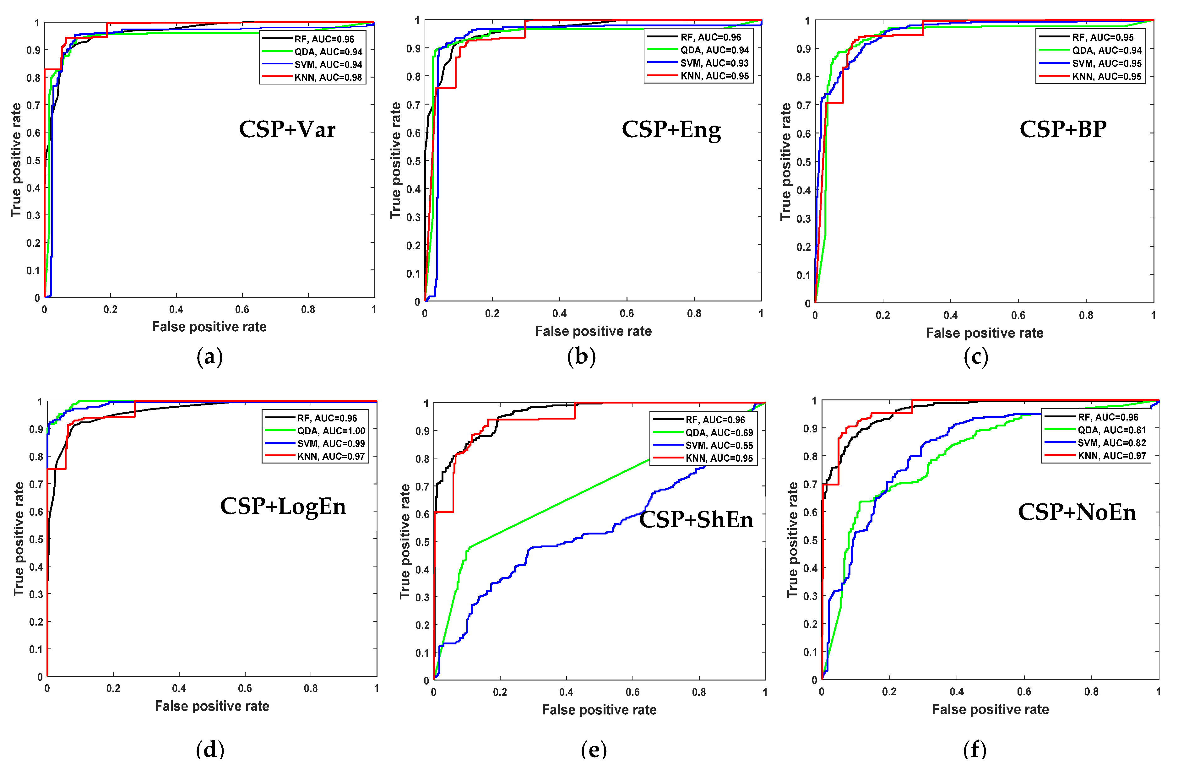
| FE Methods | Accuracy (%) | Sensitivity (%) | Specificity (%) | F-Score (%) |
|---|---|---|---|---|
| mean ± st | mean ± st | mean ± st | mean ± st | |
| CSP+Var | 96.37 ± 3.18 | 96.80 ± 4.42 | 96.16 ± 3.21 | 96.34 ± 3.15 |
| CSP+Eng | 93.23 ± 2.53 | 91.21 ± 3.27 | 95.57 ± 2.74 | 93.34 ± 2.43 |
| CSP+LBP | 93.90 ± 2.19 | 92.11 ± 3.18 | 95.96 ± 2.65 | 93.97 ± 2.15 |
| CSP+LogEn | 94.22 ± 2.96 | 93.65 ± 4.11 | 95.27 ± 4.95 | 94.19 ± 3.01 |
| CSP+ShEn | 91.91 ± 4.72 | 92.40 ± 7.00 | 91.92 ± 3.95 | 91.90 ± 4.53 |
| CSP+ThEn | 49.67 ± 2.40 | 49.53 ± 1.37 | 59.81 ± 24.68 | 64.78 ± 2.42 |
| CSP+SuEn | 50.49 ± 5.45 | 50.17 ± 4.77 | 50.76 ± 6.59 | 53.55 ± 4.63 |
| CSP+NoEn | 93.39 ± 3.31 | 92.78 ± 5.25 | 94.45 ± 3.53 | 93.44 ± 3.18 |
|
Frequency Band | FE Method | |||||
|---|---|---|---|---|---|---|
| CSP+Var | CSP+Eng | CSP+LBP | CSP+LogEn | CSP+ShEn | CSP+NoEn | |
| 4–13 Hz | 96.86 ± 2.55 | 96.52 ± 2.99 | 96.54 ± 3.13 | 98.18 ± 1.23 | 95.54 ± 2.10 | 98.18 ± 1.81 |
| 4–30 Hz | 97.36 ± 2.09 | 96.20 ± 2.21 | 97.36 ± 2.10 | 98.02 ± 1.86 | 96.87 ± 1.79 | 97.86 ± 1.91 |
| 8–30 Hz | 97.67 ± 1.58 | 97.04 ± 2.01 | 97.36 ± 1.77 | 98.85 ± 1.74 | 96.71 ± 1.54 | 97.20 ± 1.90 |
| 10–30 Hz | 98.02 ± 1.51 | 98.02 ± 1.70 | 96.87 ± 2.12 | 99.34 ± 1.15 | 95.54 ± 3.22 | 97.17 ± 2.59 |
| 12–30 Hz | 98.34 ± 1.57 | 97.85 ± 1.58 | 97.53 ± 3.03 | 99.17 ± 1.16 | 96.69 ± 2.47 | 98.18 ± 2.11 |
| 8–32 Hz | 97.53 ± 1.39 | 96.54 ± 3.07 | 96.87 ± 2.50 | 98.68 ± 1.30 | 95.39 ± 2.65 | 97.68 ± 2.50 |
| 10–32 Hz | 98.18 ± 1.65 | 97.52 ± 2.48 | 97.69 ± 1.60 | 98.85 ± 1.56 | 96.05 ± 2.59 | 98.69 ± 1.51 |
| 12–32 Hz | 98.02 ± 1.30 | 97.36 ± 1.60 | 97.17 ± 2.58 | 98.36 ± 1.73 | 97.52 ± 1.94 | 98.52 ± 1.44 |
| 14–32 Hz | 98.35 ± 1.09 | 97.52 ± 1.95 | 97.36 ± 1.96 | 98.84 ± 1.76 | 97.68 ± 2.50 | 98.35 ± 1.35 |
| 15–32 Hz | 98.68 ± 1.05 | 96.86 ± 1.99 | 97.03 ± 1.87 | 98.18 ± 1.66 | 97.20 ± 2.33 | 97.03 ± 2.44 |
| 10–25 Hz | 97.19 ± 1.77 | 96.70 ± 1.35 | 97.52 ± 2.11 | 98.18 ± 1.45 | 95.87 ± 2.85 | 97.69 ± 2.49 |
| 8–25 Hz | 97.36 ± 1.77 | 97.02 ± 2.45 | 97.52 ± 1.61 | 98.52 ± 1.21 | 96.20 ± 2.61 | 97.19 ± 2.59 |
| Reduction Number | Segment Length (Number of Segments M) | |||||
|---|---|---|---|---|---|---|
| 2 s (3032) | 4 s (1516) | 6 s (1010) | 8 s (758) | 10 s (606) | 12 s (505) | |
| 10 | 98.02 ± 1.28 | 98.55 ± 0.87 | 97.62 ± 1.34 | 97.76 ± 1.53 | 98.02 ± 1.52 | 97.82 ± 2.37 |
| 12 | 98.71 ± 0.69 | 98.61 ± 0.79 | 98.91 ± 0.87 | 98.03 ± 1.27 | 98.84 ± 1.12 | 97.82 ± 2.57 |
| 14 | 98.88 ± 0.61 | 99.04 ± 0.54 | 98.81 ± 1.30 | 98.68 ± 1.38 | 99.01 ± 1.16 | 97.22 ± 2.14 |
| 16 | 98.98 ± 0.69 | 99.14 ± 0.88 | 98.51 ± 1.07 | 98.69 ± 1.07 | 98.35 ± 1.34 | 98.42 ± 1.80 |
| 18 | 99.04 ± 0.69 | 99.34 ± 0.70 | 98.91 ± 1.19 | 98.94 ± 1.05 | 98.84 ± 1.36 | 98.81 ± 1.03 |
| 20 | 98.94 ± 0.66 | 99.41 ± 0.85 | 98.71 ± 1.05 | 98.95 ± 0.83 | 99.01 ± 1.16 | 99.21 ± 1.37 |
| 22 | 99.18 ± 0.61 | 99.08 ± 0.83 | 98.71 ± 1.15 | 98.81 ± 1.31 | 98.84 ± 1.76 | 97.81 ± 2.19 |
| 24 | 99.14 ± 0.35 | 99.27 ± 0.66 | 98.91 ± 1.19 | 98.68 ± 1.25 | 98.84 ± 1.12 | 98.22 ± 1.46 |
| 26 | 99.08 ± 0.73 | 99.14 ± 0.77 | 98.61 ± 1.42 | 99.07 ± 0.89 | 98.85 ± 1.56 | 99.01 ± 1.04 |
| 28 | 99.41 ± 0.43 | 99.14 ± 0.54 | 98.51 ± 0.96 | 99.21 ± 0.93 | 98.68 ± 1.04 | 99.20 ± 1.03 |
| 30 | 99.47 ± 0.35 | 99.01 ± 0.47 | 98.91 ± 0.73 | 98.55 ± 1.16 | 98.19 ± 1.63 | 99.00 ± 1.41 |
| 32 | 99.41 ± 0.43 | 99.08 ± 0.77 | 98.22 ± 1.46 | 98.55 ± 1.58 | 99.17 ± 1.18 | 98.42 ± 2.03 |
| Classifier | Accuracy (%) | Sensitivity (%) | Specificity (%) | F-Score (%) |
|---|---|---|---|---|
| mean ± st | mean ± st | mean ± st | mean ± st | |
| RF | 97.59 ± 0.96 | 96.96 ± 1.99 | 98.30 ± 1.10 | 97.59 ± 0.94 |
| QDA | 98.58 ± 0.97 | 98.29 ± 1.50 | 98.88 ± 0.70 | 98.58 ± 0.97 |
| SVM | 99.04 ± 0.61 | 99.14 ± 1.03 | 98.97 ± 0.85 | 98.03 ± 0.62 |
| KNN | 99.41 ± 0.43 | 99.47 ± 0.80 | 99.35 ± 0.74 | 99.40 ± 0.44 |
| FE Methods | Accuracy (%) | Sensitivity (%) | Specificity (%) | F-Score (%) |
|---|---|---|---|---|
| mean ± st | mean ± st | mean ± st | mean ± st | |
| CSP+Var | 92.87 ± 2.32 | 92.02 ± 4.11 | 94.23 ± 4.55 | 92.83 ± 2.40 |
| CSP+Eng | 89.54 ± 4.24 | 87.47 ± 6.71 | 87.47 ± 6.71 | 92.45 ± 3.95 |
| CSP+LBP | 90.21 ± 1.85 | 89.88 ± 6.31 | 91.92 ± 5.41 | 90.16 ± 1.76 |
| CSP+LogEn | 92.85 ± 2.65 | 92.22 ± 5.72 | 94.33 ± 3.93 | 92.87 ± 2.48 |
| CSP+ShEn | 90.55 ± 3.43 | 88.95 ± 2.76 | 92.34 ± 4.98 | 90.54 ± 3.49 |
| CSP+ThEn | 51.58 ± 4.08 | 50.44 ± 2.31 | 61.83 ± 31.55 | 65.34 ± 3.47 |
| CSP+SuEn | 57.36 ± 5.36 | 56.66 ± 5.31 | 58.11 ± 5.47 | 58.12 ± 4.25 |
| CSP+NoEn | 91.03 ± 3.35 | 89.68 ± 4.01 | 92.88 ± 5.27 | 91.00 ± 3.54 |
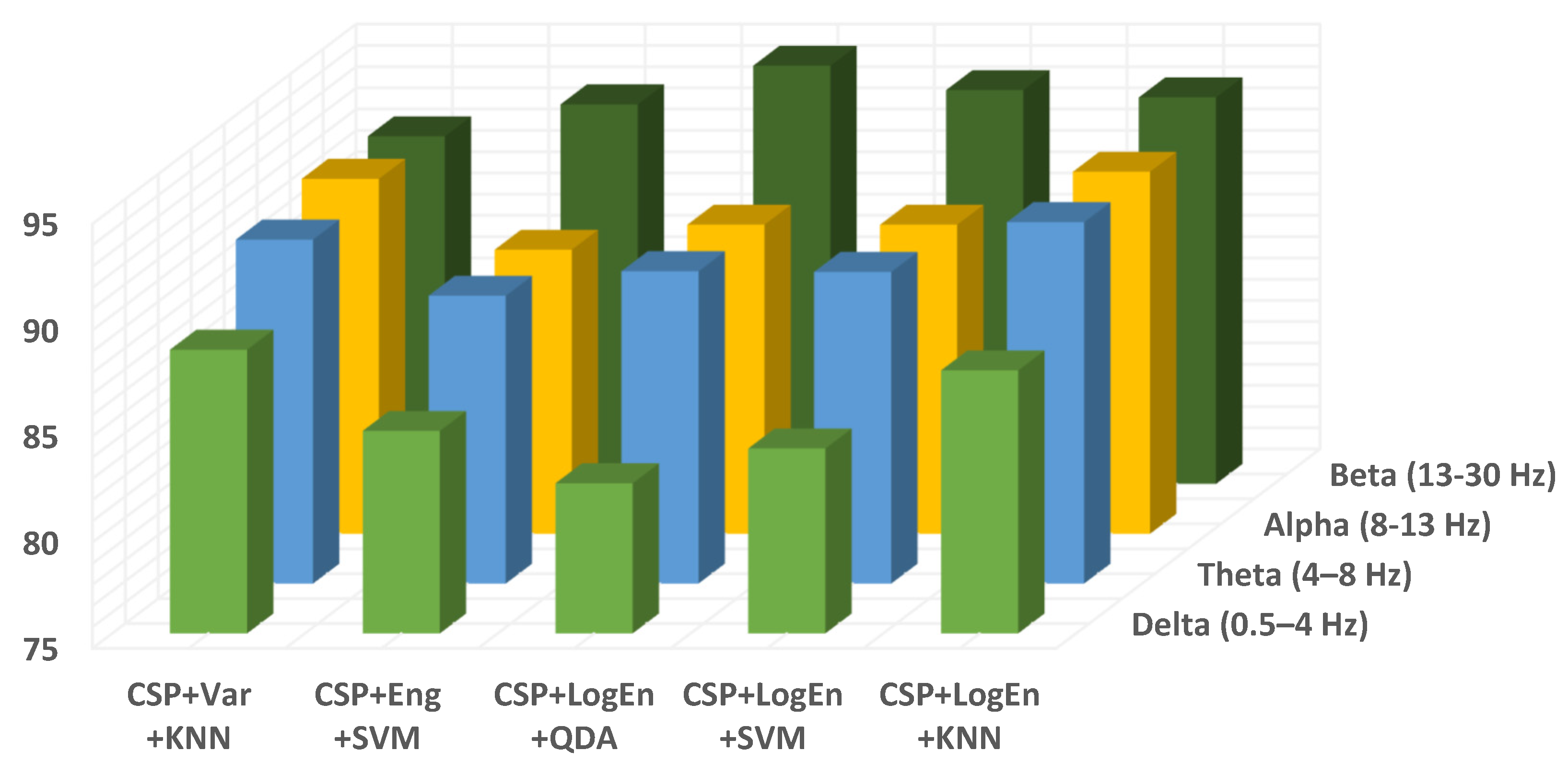
| Frequency Band | Method | ||||
|---|---|---|---|---|---|
| CSP+Var +KNN | CSP+Eng +SVM | CSP+LogEn +QDA | CSP+LogEn +SVM | CSP+LogEn +KNN | |
| 4–13 Hz | 91.54 ± 3.08 | 91.04 ± 5.20 | 92.87 ± 3.69 | 93.20 ± 2.53 | 92.20 ± 2.95 |
| 4–30 Hz | 92.37 ± 2.50 | 92.36 ± 3.16 | 95.20 ± 2.63 | 95.70 ± 1.94 | 93.20 ± 1.42 |
| 8–30 Hz | 93.05 ± 2.53 | 91.56 ± 3.97 | 94.36 ± 1.94 | 94.70 ± 2.18 | 92.21 ± 2.93 |
| 10–30 Hz | 92.87 ± 1.77 | 92.38 ± 2.81 | 94.53 ± 3.02 | 94.52 ± 2.49 | 92.21 ± 3.32 |
| 12–30 Hz | 92.70 ± 2.75 | 92.53 ± 3.37 | 95.36 ± 2.90 | 94.53 ± 1.91 | 92.88 ± 2.89 |
| 8–32 Hz | 91.55 ± 3.44 | 92.37 ± 4.32 | 94.54 ± 1.87 | 94.86 ± 1.97 | 92.88 ± 2.04 |
| 10–32 Hz | 92.04 ± 3.40 | 92.37 ± 4.24 | 95.35 ± 2.92 | 94.20 ± 3.08 | 92.19 ± 3.64 |
| 12–32 Hz | 92.20 ± 2.49 | 93.22 ± 4.32 | 95.20 ± 1.97 | 94.53 ± 2.93 | 93.54 ± 2.74 |
| 14–32 Hz | 92.54 ± 3.41 | 92.54 ± 1.15 | 95.28 ± 2.97 | 94.37 ± 2.20 | 93.04 ± 2.79 |
| 15–30 Hz | 91.39 ± 3.15 | 91.88 ± 3.99 | 95.18 ± 1.88 | 94.67 ± 2.76 | 93.85 ± 1.81 |
| 10–25 Hz | 92.04 ± 1.90 | 93.87 ± 1.74 | 95.52 ± 2.36 | 94.52 ± 2.62 | 92.20 ± 2.72 |
| 8–25 Hz | 92.05 ± 3.27 | 92.85 ± 1.63 | 95.35 ± 3.03 | 95.17 ± 2.18 | 92.51 ± 3.56 |
| Classifier | Segment Length (Number of Segments) | |||||
|---|---|---|---|---|---|---|
| 2 s (3020) | 4 s (1510) | 6 s (1006) | 8 s (755) | 10 s (603) | 12 s (503) | |
| RF | 92.25 ± 0.86 | 92.51 ± 2.46 | 92.14 ± 2.85 | 91.53 ± 3.99 | 91.53 ± 4.54 | 91.46 ± 5.14 |
| QDA | 93.54 ± 1.70 | 95.03 ± 1.72 | 94.32 ± 3.56 | 95.63 ± 2.99 | 95.19 ± 2.15 | 95.24 ± 3.12 |
| SVM | 95.00 ± 0.94 | 94.63 ± 2.64 | 94.32 ± 3.13 | 95.76 ± 2.56 | 94.53 ± 2.59 | 95.03 ± 2.14 |
| KNN | 93.38 ± 0.81 | 93.84 ± 2.25 | 93.43 ± 3.21 | 93.38 ± 3.35 | 92.87 ± 2.70 | 93.25 ± 3.41 |
| FE Methods | Accuracy (%) | Sensitivity (%) | Specificity (%) | F-Score (%) |
|---|---|---|---|---|
| mean ± st | mean ± st | mean ± st | mean ± st | |
| CSP+Var | 97.02 ± 1.06 | 97.59 ± 1.49 | 96.50 ± 1.50 | 97.02 ± 1.07 |
| CSP+Eng | 97.09 ± 0.79 | 97.46 ± 0.97 | 96.75 ± 1.19 | 97.09 ± 0.80 |
| CSP+LBP | 96.99 ± 0.44 | 96.95 ± 0.90 | 97.06 ± 1.15 | 97.00 ± 0.45 |
| CSP+LogEn | 97.52 ± 0.95 | 97.92 ± 1.01 | 97.14 ± 1.22 | 97.52 ± 0.95 |
| CSP+ShEn | 94.85 ± 1.28 | 96.32 ± 1.65 | 93.53 ± 2.16 | 94.78 ± 1.34 |
| CSP+NoEn | 96.15 ± 1.00 | 96.81 ± 2.04 | 95.58 ± 1.19 | 96.15 ± 0.96 |
| Classification Accuracy (mean ± st) | ||||||
|---|---|---|---|---|---|---|
| RF | SVM | KNN | ||||
| FE Methods | Close Eyes | Open Eyes | Close Eyes | Open Eyes | Close Eyes | Open Eyes |
| CSP+Var | 96.23 ± 1.85 | 96.54 ± 1.02 | 97.17 ± 1.43 | 97.35 ± 0.92 | 98.24 ± 0.77 | 98.52 ± 0.88 |
| CSP+Eng | 96.99 ± 1.95 | 96.73 ± 0.72 | 97.05 ± 1.19 | 97.41 ± 2.05 | 98.12 ± 1.19 | 98.02 ± 1.04 |
| CSP+LBP | 96.61 ± 1.19 | 97.04 ± 1.53 | 96.92 ± 1.43 | 96.85 ± 1.68 | 98.05 ± 1.00 | 98.40 ± 0.83 |
| CSP+LogEn | 97.18 ± 1.19 | 98.02 ± 0.96 | 98.12 ± 1.11 | 98.58 ± 1.01 | 98.81 ± 1.00 | 99.01 ± 0.93 |
| Classification Accuracy (mean ± st) | ||||||
|---|---|---|---|---|---|---|
| RF | SVM | KNN | ||||
| FE Methods | Close Eyes | Open Eyes | Close Eyes | Open Eyes | Close Eyes | Open Eyes |
| CSP+Var | 96.80 ± 1.45 | 96.91 ± 1.29 | 97.10 ± 1.27 | 98.12 ± 1.26 | 98.58 ± 0.87 | 98.85 ± 0.97 |
| CSP+Eng | 97.35 ± 1.54 | 97.58 ± 1.25 | 97.66 ± 1.59 | 97.76 ± 1.11 | 98.33 ± 1.13 | 98.18 ± 0.57 |
| CSP+LBP | 97.66 ± 1.19 | 97.45 ± 1.21 | 97.10 ± 0.97 | 97.58 ± 1.59 | 98.21 ± 0.79 | 98.42 ± 1.28 |
| CSP+LogEn | 97.29 ± 0.83 | 98.00 ± 0.57 | 97.54 ± 1.33 | 98.12 ± 0.73 | 98.77 ± 0.71 | 98.85 ± 0.54 |
| Classification Accuracy (mean ± st) | ||||||
|---|---|---|---|---|---|---|
| RF | SVM | KNN | ||||
| FE Methods | Close Eyes | Open Eyes | Close Eyes | Open Eyes | Close Eyes | Open Eyes |
| CSP+Var | 95.82 ± 1.75 | 94.73 ± 1.57 | 97.88 ± 0.96 | 96.61 ± 1.28 | 98.36 ± 1.11 | 98.61 ± 0.50 |
| CSP+Eng | 96.67 ± 0.91 | 95.94 ± 1.40 | 97.52 ± 1.01 | 95.27 ± 1.61 | 98.79 ± 1.03 | 98.18 ± 0.70 |
| CSP+LBP | 97.27 ± 0.77 | 95.88 ± 1.14 | 97.88 ± 1.04 | 95.09 ± 2.70 | 98.79 ± 1.07 | 98.24 ± 0.60 |
| CSP+LogEn | 95.88 ± 1.53 | 94.61 ± 2.48 | 97.82 ± 1.04 | 96.73 ± 1.22 | 98.97 ± 0.70 | 98.73 ± 0.78 |
| Reference | FE Methods | Classifier(s) | Dataset | Classification Type | Classification Accuracy (%) |
|---|---|---|---|---|---|
| Yuvaraj, R. et al. (2018) | Higher-order spectra (HOS) | DT, KNN, FKNN, NB, PNN, SVM | Malaysian dataset | Off–PD vs. HC | 90.6–99.6 |
| Oh, S. L. et al. (2020) | ---- | 13 layer CNN | Malaysian dataset | Off–PD vs. HC | 88.25 |
| Shah S. A. et al. (2020) | ---- | CNN+LSTM | UNM dataset | Off–PD vs. On–PD | 99.2 |
| Fahim A. et al. (2020) | PSD | Hyperplanes | UNM dataset | Off–PD vs. HC | 85.3 |
| Lee S. et al. (2021) | -- | CNN+RNN | Own dataset | Off–PD vs. HC | 99.2 |
| Smith K. K. et al. (2021) | WT+statistical measures | SVM | SanDiego dataset | Off–PD vs. HC On–PD vs. HC | 96.13 97.65 |
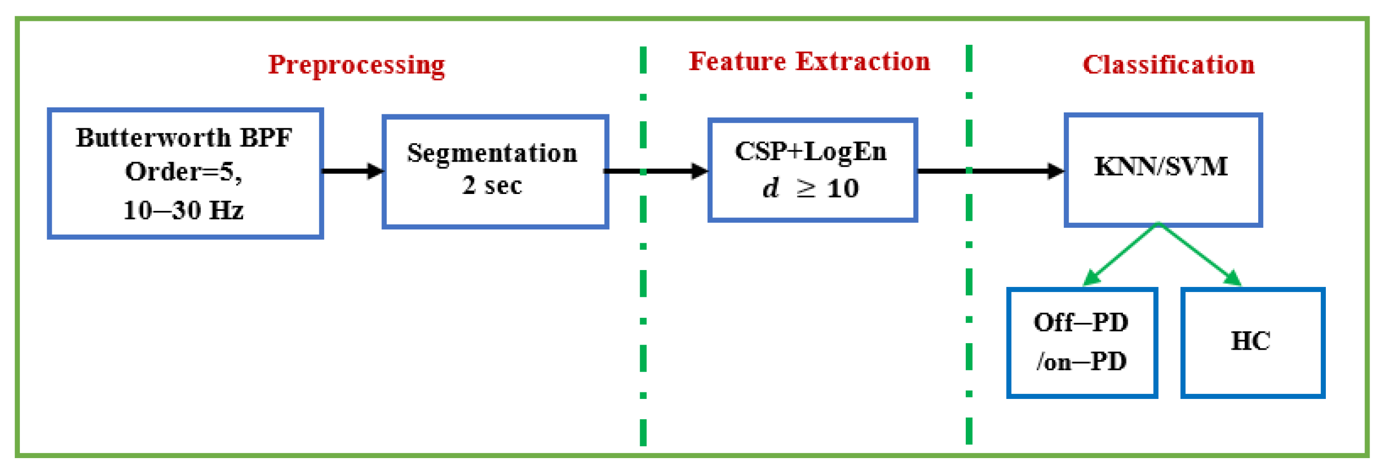
| Present study | CSP+LogEn | KNN | UNM dataset (Close/open) | Off–PD vs. on–PD On–PD vs. HC Off–PD vs. HC | 98.73/98.97 98.77/98.85 98.81/99.01 |
| CSP+LogEn | KNN SVM KNN | SanDiego dataset | Off–PD vs. on–PD On–PD vs. HC Off–PD vs. HC | 97.52 95.76 99.41 |
Publisher’s Note: MDPI stays neutral with regard to jurisdictional claims in published maps and institutional affiliations. |
© 2022 by the authors. Licensee MDPI, Basel, Switzerland. This article is an open access article distributed under the terms and conditions of the Creative Commons Attribution (CC BY) license (https://creativecommons.org/licenses/by/4.0/).
Share and Cite
Aljalal, M.; Aldosari, S.A.; AlSharabi, K.; Abdurraqeeb, A.M.; Alturki, F.A. Parkinson’s Disease Detection from Resting-State EEG Signals Using Common Spatial Pattern, Entropy, and Machine Learning Techniques. Diagnostics 2022, 12, 1033. https://doi.org/10.3390/diagnostics12051033
Aljalal M, Aldosari SA, AlSharabi K, Abdurraqeeb AM, Alturki FA. Parkinson’s Disease Detection from Resting-State EEG Signals Using Common Spatial Pattern, Entropy, and Machine Learning Techniques. Diagnostics. 2022; 12(5):1033. https://doi.org/10.3390/diagnostics12051033
Chicago/Turabian StyleAljalal, Majid, Saeed A. Aldosari, Khalil AlSharabi, Akram M. Abdurraqeeb, and Fahd A. Alturki. 2022. "Parkinson’s Disease Detection from Resting-State EEG Signals Using Common Spatial Pattern, Entropy, and Machine Learning Techniques" Diagnostics 12, no. 5: 1033. https://doi.org/10.3390/diagnostics12051033
APA StyleAljalal, M., Aldosari, S. A., AlSharabi, K., Abdurraqeeb, A. M., & Alturki, F. A. (2022). Parkinson’s Disease Detection from Resting-State EEG Signals Using Common Spatial Pattern, Entropy, and Machine Learning Techniques. Diagnostics, 12(5), 1033. https://doi.org/10.3390/diagnostics12051033