
A Novel Computer-Aided Diagnostic System for Early Detection of Diabetic Retinopathy Using 3D-OCT Higher-Order Spatial Appearance Model

 ,
,  ,
,  , ,
, ,  ,
, 
Abstract
:1. Introduction
Related Work
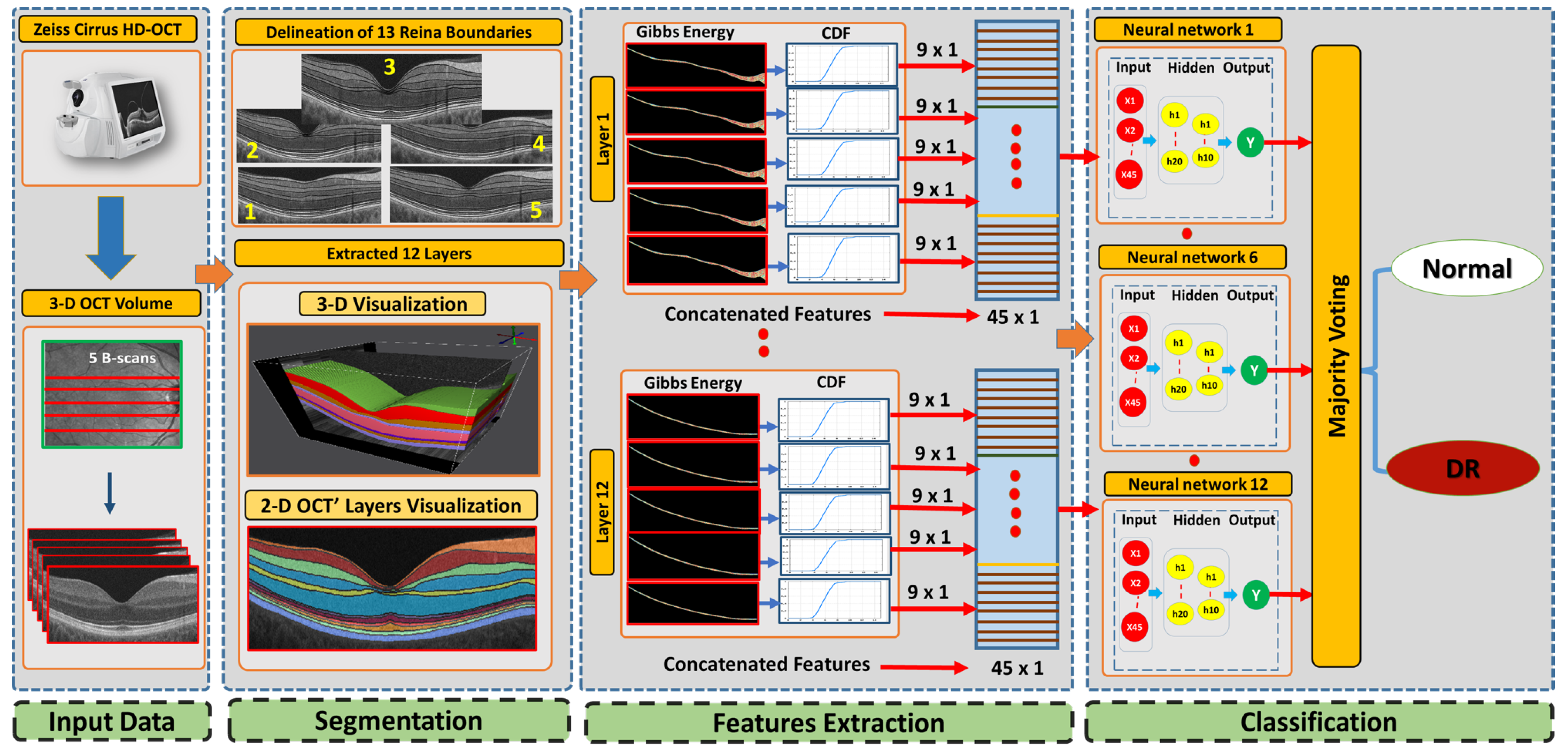
- Each layer of the OCT is analyzed separately and is classified for local and individualized analyses. In the following step, the decision of the individual layers is combined into a global diagnosis.
- Our system integrates incorporates a 3D-MGRF model, which is in place of using a 1st-order reflectivity.
- To improve the descriptive power of the extracted features, a statistical approach is used (i.e., CDF percentile).
- The CDF percentile values are fed into an ANN to get the final diagnosis of the 3D OCT volume.
2. Method
2.1. 3D-OCT Volume Segmentation
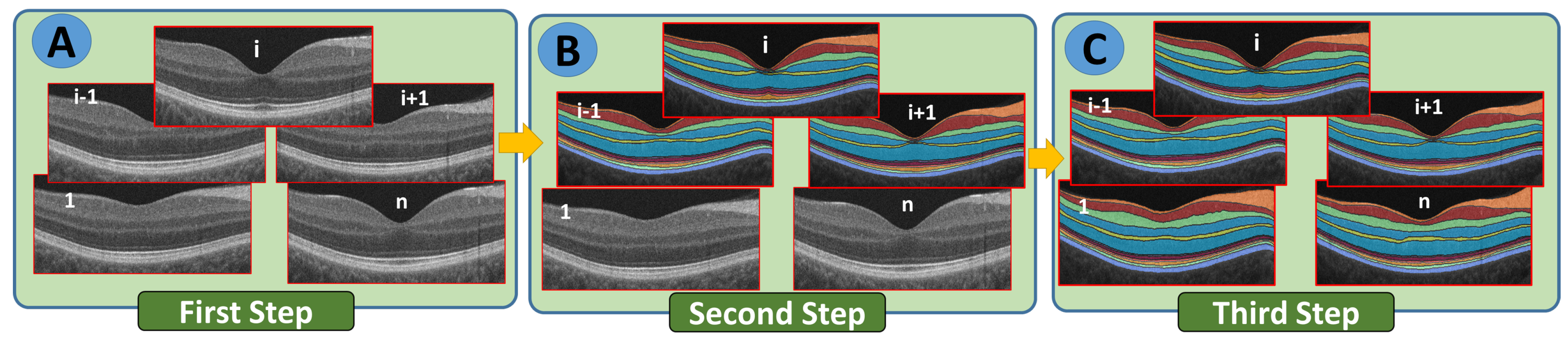
- Step 1: The B-scans are matched to a shape database built by the expert. The database contains manually segmented foveal B-scans representing normal and diseased retinas.
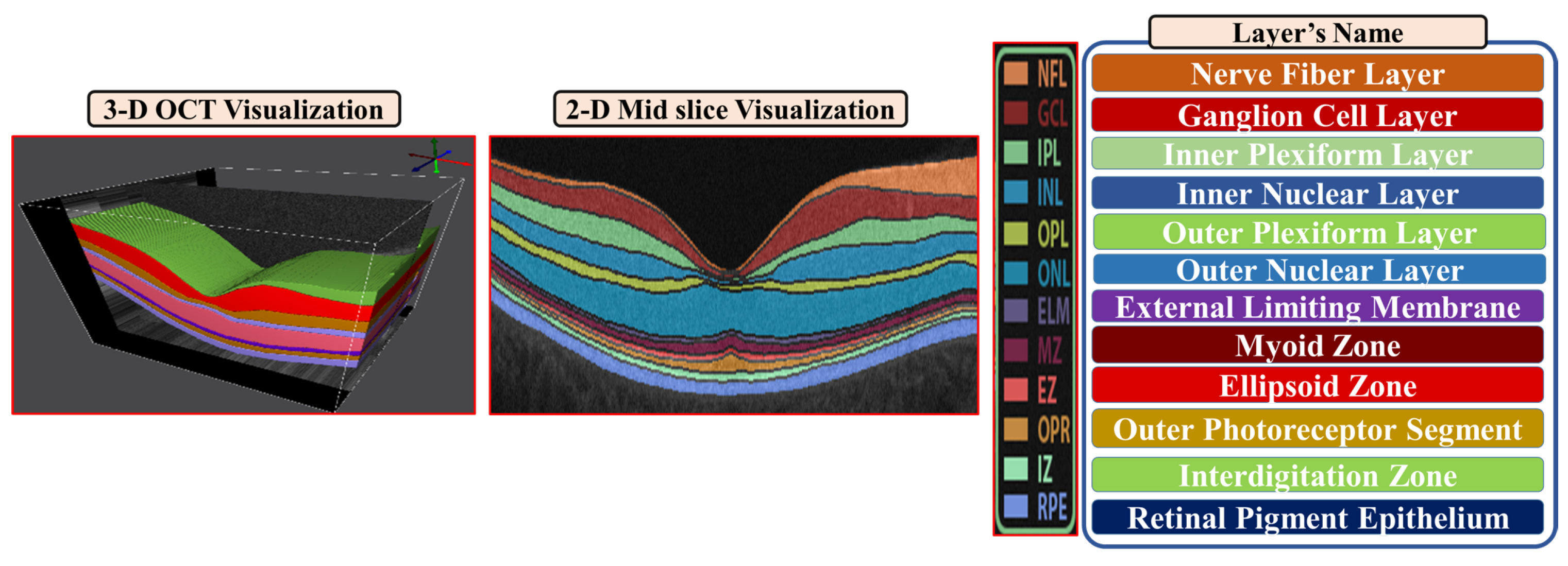
- Step 2: The second step is to divide the region between the vitreous and choroid into twelve distinct segments based on the interaction model for shape, intensity, and spatial interactions.
- Step 3: In the third step, the unprocessed B-scans are used as prior shape models in the process of segmenting each segmented B-scan.
- Step 4: The prior shape models are refined to obtain the final segmentation
| Algorithm 1: Prior shape propagation algorithm |
|
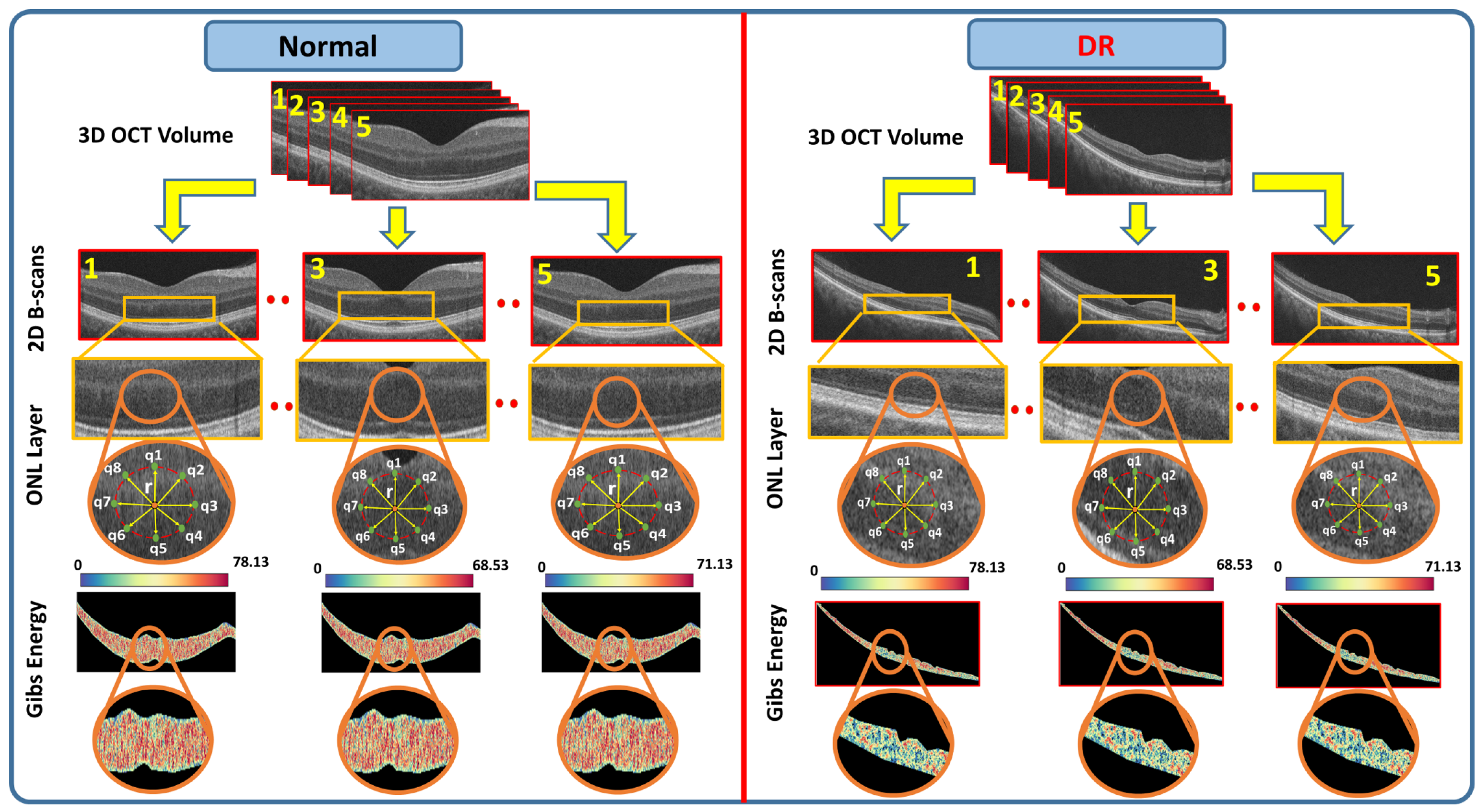
2.2. Feature Extraction
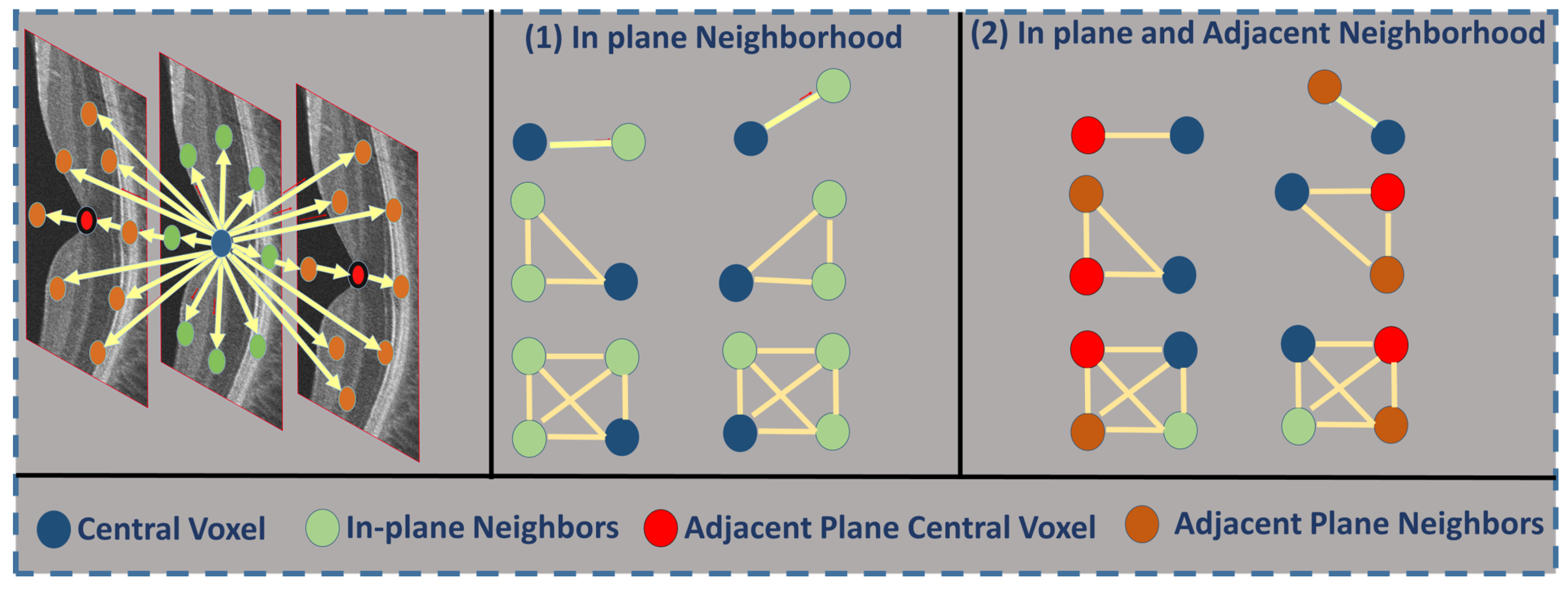
- is a grayscale image on the discrete domain with pixel values in .
- is a set of -offsets specifying the pairwise neighborhood system.
- C is the graph of pixel interactions on R; the neighborhood system for pixel is the set of pairs .
- is the Gibbs potential associated with neighborhood .
| Algorithm 2: Extracting the feature vector using 3D-MGRF |
|
2.3. Classification System
| Algorithm 3: ANN training |
|
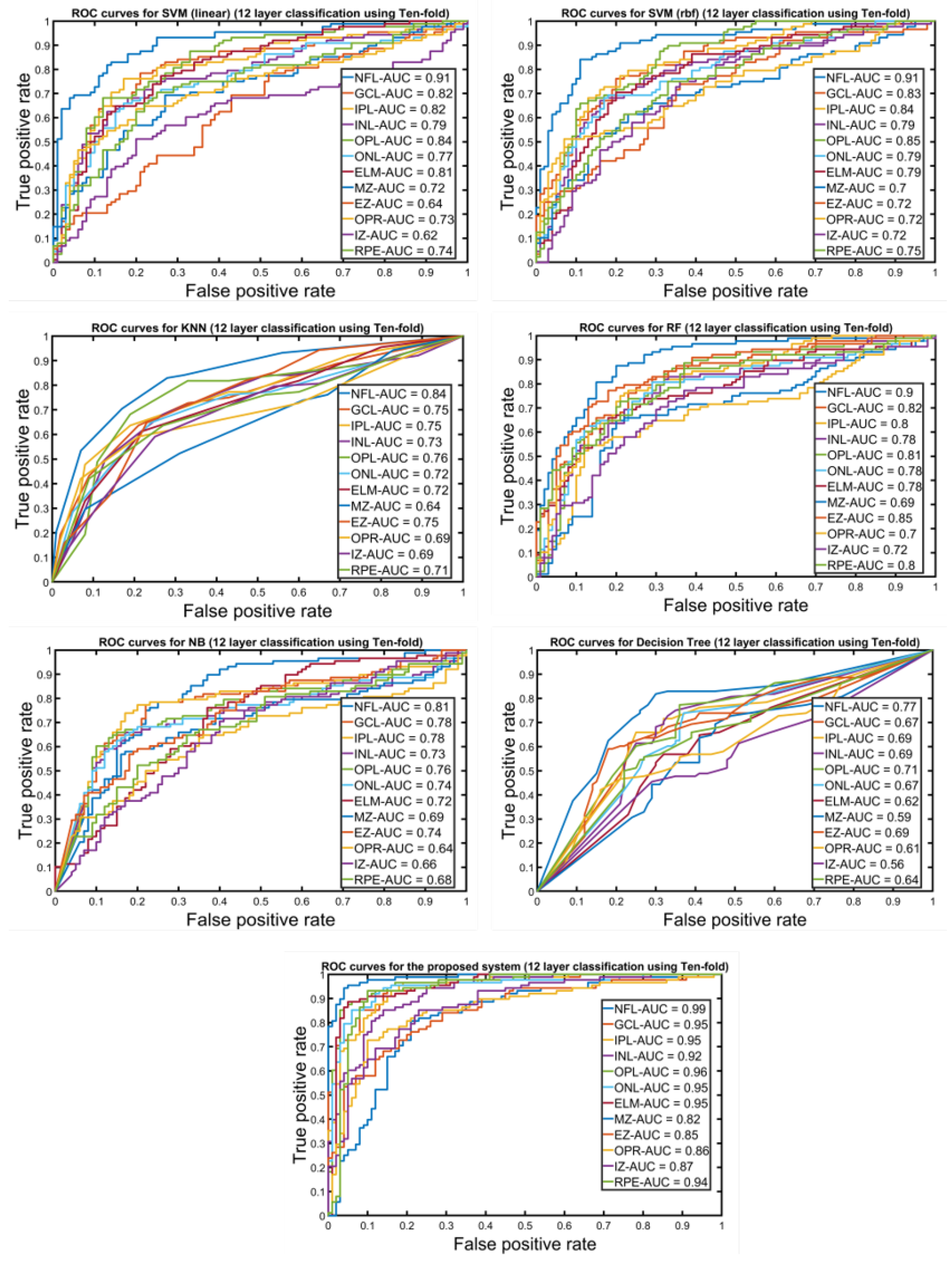
3. Experimental Results
4. Conclusions and Future Work
Author Contributions
Funding
Institutional Review Board Statement
Informed Consent Statement
Data Availability Statement
Conflicts of Interest
References
- Saeedi, P.; Petersohn, I.; Salpea, P.; Malanda, B.; Karuranga, S.; Unwin, N.; Colagiuri, S.; Guariguata, L.; Motala, A.; Ogurtsova, K.; et al. Global and regional diabetes prevalence estimates for 2019 and projections for 2030 and 2045: Results from the International Diabetes Federation Diabetes Atlas, 9th edition. Diabetes Res. Clin. Pract. 2019, 157, 107843. [Google Scholar] [CrossRef] [PubMed] [Green Version]
- Centers for Disease Control and Prevention. Available online: https://www.cdc.gov/visionhealth/pdf/factsheet.pdf (accessed on 1 December 2021).
- Foeady, A.Z.; Novitasari, D.C.R.; Asyhar, A.H.; Firmansjah, M. Automated Diagnosis System of Diabetic Retinopathy Using GLCM Method and SVM Classifier. In Proceedings of the 2018 5th International Conference on Electrical Engineering, Computer Science and Informatics (EECSI), Malang, Indonesia, 16–18 October 2018; pp. 154–160. [Google Scholar]
- Rahim, S.S.; Palade, V.; Shuttleworth, J.; Jayne, C. Automatic screening and classification of diabetic retinopathy and maculopathy using fuzzy image processing. Brain Inform. 2016, 3, 249–267. [Google Scholar] [CrossRef] [PubMed]
- Sandhu, H.S.; Elmogy, M.; Sharafeldeen, A.T.; Elsharkawy, M.; Eladawi, N.; Eltanboly, A.; Shalaby, A.; Keynton, R.; El-Baz, A. Automated Diagnosis of Diabetic Retinopathy Using Clinical Biomarkers, Optical Coherence Tomography, and Optical Coherence Tomography Angiography. Am. J. Ophthalmol. 2020, 216, 201–206. [Google Scholar] [CrossRef] [PubMed]
- Bernardes, R.; Serranho, P.; Santos, T.; Gonçalves, V.; Cunha-Vaz, J. Optical Coherence Tomography: Automatic Retina Classification through Support Vector Machines. Eur. Ophthalmic Rev. 2012, 6, 200–203. Available online: https://repositorioaberto.uab.pt/handle/10400.2/2765 (accessed on 29 November 2021). [CrossRef] [Green Version]
- Maetschke, S.; Antony, B.; Ishikawa, H.; Wollstein, G.; Schuman, J.; Garnavi, R. A feature agnostic approach for glaucoma detection in OCT volumes. PLoS ONE 2019, 14, e0219126. [Google Scholar] [CrossRef]
- Ko, C.E.; Chen, P.H.; Liao, W.M.; Lu, C.K.; Lin, C.H.; Liang, J.W. Using A Cropping Technique or Not: Impacts on SVM-based AMD Detection on OCT Images. In Proceedings of the 2019 IEEE International Conference on Artificial Intelligence Circuits and Systems, Hsinchu, Taiwan, 18–20 March 2019; pp. 199–200. [Google Scholar]
- Serener, A.; Serte, S. Dry and Wet Age-Related Macular Degeneration Classification Using OCT Images and Deep Learning. In Proceedings of the 2019 Scientific Meeting on Electrical-Electronics & Biomedical Engineering and Computer Science (EBBT), Istanbul, Turkey, 24–26 April 2019; pp. 1–4. [Google Scholar]
- Pekala, M.J.; Joshi, N.J.; Alvin Liu, T.Y.; Bressler, N.M.; Cabrera DeBuc, D.; Burlina, P. Deep learning based retinal OCT segmentation. Comput. Biol. Med. 2019, 114, 103445. [Google Scholar] [CrossRef] [Green Version]
- Mohammed, S.; Li, T.; Chen, X.D.; Warner, E.; Shankar, A.; Abalem, M.F.; Jayasundera, T.; Gardner, T.W.; Rao, A. Density-based classification in diabetic retinopathy through thickness of retinal layers from optical coherence tomography. Sci. Rep. 2020, 10, 15937. [Google Scholar] [CrossRef]
- Alam, M.; Zhang, Y.; Lim, J.; Chan, R.; Yang, M.; Yao, X. Quantitative optical coherence tomography angiography features for objective classification and staging of diabetic retinopathy. Retina 2018, 40, 322–332. [Google Scholar] [CrossRef]
- Alsaih, K.; Lemaitre, G.; Rastgoo, M.; Massich, J.; Sidibé, D. Machine learning techniques for diabetic macular edema (DME) classification on SD-OCT images. BioMed. Eng. Online 2017, 16, 68. [Google Scholar] [CrossRef] [Green Version]
- Lemaître, G.; Rastgoo, M.; Massich, J.; Cheung, C.; Wong, T.Y.; Lamoureux, E.; Milea, D.; Meriaudeau, F.; Sidibé, D. Classification of SD-OCT Volumes using Local Binary Patterns: Experimental Validation for DME Detection. J. Ophthalmol. 2016, 2016, 3298606. [Google Scholar] [CrossRef] [Green Version]
- Ibrahim, M.; Fathalla, K.; Youssef, S. HyCAD-OCT: A Hybrid Computer-Aided Diagnosis of Retinopathy by Optical Coherence Tomography Integrating Machine Learning and Feature Maps Localization. Appl. Sci. 2020, 10, 4716. [Google Scholar] [CrossRef]
- Ghazal, M.; Ali, S.S.; Mahmoud, A.H.; Shalaby, A.M.; El-Baz, A. Accurate Detection of Non-Proliferative Diabetic Retinopathy in Optical Coherence Tomography Images Using Convolutional Neural Networks. IEEE Access 2020, 8, 34387–34397. [Google Scholar] [CrossRef]
- Elsharkawy, M.; Elrazzaz, M.; Ghazal, M.; Alhalabi, M.; Soliman, A.; Mahmoud, A.; El-Daydamony, E.; Atwan, A.; Thanos, A.; Sandhu, A.; et al. Role of Optical Coherence Tomography Imaging in Predicting Progression of Age-Related Macular Disease: A Survey. Diagnostics 2021, 11, 2313. [Google Scholar] [CrossRef] [PubMed]
- Banerjee, I.; Sisternes, L.; Hallak, J.; Leng, T.; Osborne, A.; Durbin, M.; Rubin, D. A Deep-learning Approach for Prognosis of Age-Related Macular Degeneration Disease using SD-OCT Imaging Biomarkers. arXiv 2019, arXiv:1902.10700. [Google Scholar]
- An, G.; Omodaka, K.; Hashimoto, K.; Tsuda, S.; Shiga, Y.; Takada, N.; Kikawa, T.; Yokota, H.; Akiba, M.; Nakazawa, T. Glaucoma Diagnosis with Machine Learning Based on Optical Coherence Tomography and Color Fundus Images. J. Healthc. Eng. 2019, 2019, 4061313. [Google Scholar] [CrossRef]
- Mateen, M.; Wen, J.; Hassan, M.; Nasrullah, N.; Sun, S.; Hayat, S. Automatic Detection of Diabetic Retinopathy: A Review on Datasets, Methods and Evaluation Metrics. IEEE Access 2020, 8, 48784–48811. [Google Scholar] [CrossRef]
- Shankar, K.; Wahab Sait, A.R.; Gupta, D.; Lakshmanaprabu, S.K.; Khanna, A.; Mohan Pandey, H. Automated detection and classification of fundus diabetic retinopathy images using synergic deep learning model. Pattern Recognit. Lett. 2020, 133, 210–216. [Google Scholar] [CrossRef]
- Cao, K.; Xu, J.; Zhao, W.Q. Artificial intelligence on diabetic retinopathy diagnosis: An automatic classification method based on grey level co-occurrence matrix and naive Bayesian model. Int. J. Ophthalmol. 2019, 12, 1158–1162. [Google Scholar] [CrossRef]
- Ng, W.S.; Mahmud, W.M.H.W.; Huong, A.K.C.; Kairuddin, W.N.H.W.; Gan, H.S.; Izaham, R.M.A.R. Computer Aided Diagnosis of Eye Disease for Diabetic Retinopathy. J. Phys. Conf. Ser. IOP Publ. 2019, 1372, 012030. [Google Scholar] [CrossRef] [Green Version]
- Bannigidad, P.; Deshpande, A. Exudates detection from digital fundus images using glcm features with decision tree classifier. In International Conference on Recent Trends in Image Processing and Pattern Recognition; Springer: Berlin/Heidelberg, Germany, 2018; pp. 245–257. [Google Scholar]
- Rashed, N.; Ali, S.; Dawood, A. Diagnosis retinopathy disease using GLCM and ANN. J. Theor. Appl. Inf. Technol. 2018, 96, 6028–6040. [Google Scholar]
- Giraddi, S.; Pujari, J.; Seeri, S. Role of GLCM Features in Identifying Abnormalities in the Retinal Images. Int. J. Image Graph. Signal Process. 2015, 7, 45–51. [Google Scholar] [CrossRef] [Green Version]
- Le, D.; Alam, M.; Yao, C.; Lim, J.; Chan, R.; Toslak, D.; Yao, X. Transfer Learning for Automated OCTA Detection of Diabetic Retinopathy. Transl. Vis. Sci. Technol. 2020, 9, 35. [Google Scholar] [CrossRef] [PubMed]
- Heisler, M.; Karst, S.; Lo, J.; Mammo, Z.; Yu, T.; Warner, S.; Maberley, D.; Beg, M.F.; Navajas, E.; Sarunic, M. Ensemble Deep Learning for Diabetic Retinopathy Detection Using Optical Coherence Tomography Angiography. Transl. Vis. Sci. Technol. 2020, 9, 20. [Google Scholar] [CrossRef] [PubMed] [Green Version]
- Sharafeldeen, A.; Elsharkawy, M.; Khalifa, F.; Soliman, A.; Ghazal, M.; AlHalabi, M.; Yaghi, M.; Alrahmawy, M.; Elmougy, S.; Sandhu, H.; et al. Precise higher-order reflectivity and morphology models for early diagnosis of diabetic retinopathy using OCT images. Sci. Rep. 2021, 11, 4730. [Google Scholar] [CrossRef] [PubMed]
- Elsharkawy, M.; Sharafeldeen, A.; Soliman, A.; Khalifa, F.; Widjajahakim, R.; Switala, A.; Elnakib, A.; Schaal, S.; Sandhu, H.; Seddon, J.; et al. Automated diagnosis and grading of dry age-related macular degeneration using optical coherence tomography imaging. Investig. Ophthalmol. Vis. Sci. 2021, 62, 107. [Google Scholar]
- Sleman, A.A.; Soliman, A.; Elsharkawy, M.; Giridharan, G.; Ghazal, M.; Sandhu, H.; Schaal, S.; Keynton, R.; Elmaghraby, A.; El-Baz, A. A novel 3D segmentation approach for extracting retinal layers from optical coherence tomography images. Med. Phys. 2021, 48, 1584–1595. [Google Scholar] [CrossRef]
- El-Baz, A.; Gimel’farb, G.; Suri, J.S. Stochastic Modeling for Medical Image Analysis; CRC Press: Boca Raton, FL, USA, 2016. [Google Scholar] [CrossRef]
- ZEISS. CIRRUS HD-OCT 5000. Available online: https://www.zeiss.com/meditec/us/customer-care/customer-care-for-ophthalmology-optometry/quick-help-for-cirrus-hd-oct-5000.html (accessed on 25 October 2020).
- Krizhevsky, A.; Sutskever, I.; Hinton, G.E. Imagenet classification with deep convolutional neural networks. Adv. Neural Inf. Process. Syst. 2012, 25, 1097–1105. [Google Scholar] [CrossRef]
- He, K.; Zhang, X.; Ren, S.; Sun, J. Deep residual learning for image recognition. In Proceedings of the IEEE Conference on Computer Vision and Pattern Recognition, Las Vegas, NV, USA, 27–30 June 2016; pp. 770–778. [Google Scholar]
- Szegedy, C. Rethinking the inception architecture for computer vision. In Proceedings of the IEEE Conference on Computer Vision and Pattern Recognition, Las Vegas, NV, USA, 27–30 June 2016; pp. 2818–2826. [Google Scholar]

| Layer | Four Fold | Five Fold | Ten Fold | Test Set | ||||||||
|---|---|---|---|---|---|---|---|---|---|---|---|---|
| Acc. | Sens. | Spec. | Acc. | Sens. | Spec. | Acc. | Sens. | Spec. | Acc. | Sens. | Spec. | |
| NFL | 91.25% | 90.82% | 92.95% | 93.89% | 94.24% | 93.94% | 95.69% | 94.55% | 96.69% | 91% | 89.45% | 91.30% |
| GCL | 79.88% | 75.93% | 88.47% | 86.45% | 86.23% | 85.37% | 89.69% | 97.48% | 81.93% | 80.35% | 88.23% | 68.18% |
| IPL | 80.81% | 74.96% | 87.98% | 82.90% | 81.51% | 82.15% | 88.78% | 90.42% | 87.70% | 69.64% | 70.58% | 68.18% |
| INL | 87.96% | 85.70% | 90.19% | 90.75% | 89.73% | 90.98% | 89.60% | 87.15% | 87.98% | 85.71% | 85.29% | 86.36% |
| OPL | 84.60% | 84.19% | 83.69% | 92.36% | 94.89% | 87.96% | 87.87% | 91.83% | 87.94% | 80.35% | 76.47% | 86.36% |
| ONL | 84% | 82.99% | 82.64% | 74.80% | 71.97% | 80.19% | 91.93% | 90.84% | 90.80% | 82.14% | 91.17% | 68.18% |
| ELM | 80.70% | 78.36% | 80.63% | 84.87% | 80.96% | 87.60% | 80.75% | 81.69% | 81.96% | 76.78% | 73.52% | 81.81% |
| MZ | 73.21% | 74.97% | 69.87% | 74.60% | 76.40% | 71.60% | 76.47% | 78.41% | 70.94% | 66.07% | 70.58% | 59.09% |
| EZ | 77.59% | 77.32% | 78.56% | 77.60% | 78.90% | 76.85% | 77.11% | 76.56% | 78.13% | 71.42% | 76.47% | 63.63% |
| OPR | 75.12% | 81.32% | 69.74% | 77.98% | 78.87% | 73.61% | 76.80% | 73.72% | 84.68% | 58.92% | 94.11% | 63.60% |
| IZ | 75.56% | 73.89% | 73.77 | 72.87% | 80.41% | 67.35% | 86.24% | 82.95% | 90.55% | 67.85% | 76.47% | 54.54% |
| RPE | 83.98% | 80.69% | 88.63% | 87.12% | 87.54% | 86.90% | 90.21% | 86.65% | 92.99% | 75% | 85.29% | 59.09% |
| Majority Voting | 90.56% | 98.63% | 86.98% | 93.11% | 96.63% | 86.98% | 96.88% | 97.89% | 95.27% | 87.50% | 96.50% | 82.39% |
| Classifiers | Four Fold | Five Fold | Ten Fold | ||||||
|---|---|---|---|---|---|---|---|---|---|
| Acc. | Sens. | Spec. | Acc. | Sens. | Spec. | Acc. | Sens. | Spec. | |
| SVM (Linear) | 77.66% | 91% | 62.50% | 76.59% | 92% | 59.09% | 77.45% | 91.25% | 64.12% |
| SVM (rbf) | 75.53% | 88% | 61.40% | 76.06% | 89% | 61.30% | 76.06% | 88% | 62.50% |
| Logistic Regression | 72.87% | 86% | 57.95% | 78.19% | 88% | 67.05% | 81.91% | 91% | 71.59% |
| Naive Bayes | 78.72% | 74.59% | 86.36% | 71.27% | 92% | 47.72% | 72.96% | 92.68% | 52.48% |
| KNN | 70.74% | 92% | 46.60% | 77.12% | 90% | 62.50% | 78.16% | 91.97% | 62.10% |
| Random Forest | 78.19% | 88% | 67% | 77.65% | 89% | 64.77% | 79.54% | 88.36% | 66.17% |
| Decision Tree | 72.87% | 86% | 57.95% | 78.19% | 88% | 67.05% | 81.91% | 91% | 71.59% |
| Proposed System | 90.56% | 98.63% | 86.98% | 93.11% | 96.63% | 86.98% | 96.88% | 97.89% | 95.27% |
| Classifiers | Four Fold | Five Fold | Ten Fold | ||||||
|---|---|---|---|---|---|---|---|---|---|
| Acc. | Sens. | Spec. | Acc. | Sens. | Spec. | Acc. | Sens. | Spec. | |
| ResNet50 [35] | 89.12% | 97.75% | 85.10% | 90.91% | 95.63% | 85.14% | 94.90% | 92.8% | 90.21% |
| AlexNet [34] | 88.87% | 95.74% | 88.37% | 89.65% | 93% | 85.90% | 92.33% | 93.54% | 91.90% |
| InceptionV3 [36] | 89% | 96.34% | 89.30% | 90.53% | 94.67% | 84.30% | 95.60% | 96.33% | 94.99% |
| Proposed System | 90.56% | 98.63% | 86.98% | 93.11% | 96.63% | 86.98% | 96.88% | 97.89% | 95.27% |
Publisher’s Note: MDPI stays neutral with regard to jurisdictional claims in published maps and institutional affiliations. |
© 2022 by the authors. Licensee MDPI, Basel, Switzerland. This article is an open access article distributed under the terms and conditions of the Creative Commons Attribution (CC BY) license (https://creativecommons.org/licenses/by/4.0/).
Share and Cite
Elsharkawy, M.; Sharafeldeen, A.; Soliman, A.; Khalifa, F.; Ghazal, M.; El-Daydamony, E.; Atwan, A.; Sandhu, H.S.; El-Baz, A. A Novel Computer-Aided Diagnostic System for Early Detection of Diabetic Retinopathy Using 3D-OCT Higher-Order Spatial Appearance Model. Diagnostics 2022, 12, 461. https://doi.org/10.3390/diagnostics12020461
Elsharkawy M, Sharafeldeen A, Soliman A, Khalifa F, Ghazal M, El-Daydamony E, Atwan A, Sandhu HS, El-Baz A. A Novel Computer-Aided Diagnostic System for Early Detection of Diabetic Retinopathy Using 3D-OCT Higher-Order Spatial Appearance Model. Diagnostics. 2022; 12(2):461. https://doi.org/10.3390/diagnostics12020461
Chicago/Turabian StyleElsharkawy, Mohamed, Ahmed Sharafeldeen, Ahmed Soliman, Fahmi Khalifa, Mohammed Ghazal, Eman El-Daydamony, Ahmed Atwan, Harpal Singh Sandhu, and Ayman El-Baz. 2022. "A Novel Computer-Aided Diagnostic System for Early Detection of Diabetic Retinopathy Using 3D-OCT Higher-Order Spatial Appearance Model" Diagnostics 12, no. 2: 461. https://doi.org/10.3390/diagnostics12020461
APA StyleElsharkawy, M., Sharafeldeen, A., Soliman, A., Khalifa, F., Ghazal, M., El-Daydamony, E., Atwan, A., Sandhu, H. S., & El-Baz, A. (2022). A Novel Computer-Aided Diagnostic System for Early Detection of Diabetic Retinopathy Using 3D-OCT Higher-Order Spatial Appearance Model. Diagnostics, 12(2), 461. https://doi.org/10.3390/diagnostics12020461