1. Introduction
Computed tomography (CT) has been one of the most common and widespread imaging techniques used in the clinic for the last few decades. There is increasing interest in a more advanced CT technique known as dual-energy CT (DECT) or spectral CT that enables additional material or tissue characterization beyond what is possible with conventional CT. In conventional CT, X-rays are emitted at a certain level of energy, whereas in DECT, they are emitted at two separate energy levels, which brings important benefits as compared to standard CT. First, since different materials can have different attenuation coefficients at different energy levels, DECT allows for the separation of materials with different atomic numbers. In particular, DECT enables the computation of image attenuation levels at multiple effective energy levels. This results in the association of a decay curve with each reconstructed image voxel, representing energy-dependent changes in attenuation at that body location. Conventional CT imaging is the first-line modality for the clinical evaluation of many different types of known or suspected cancers in adults [
1]. However, because of the properties described above, there has been an increased interest in the use of DECT in oncology in recent years, as it provides a new and exciting way of characterizing tumors as well as their surrounding tissues.
Current expert evaluation of CT scans of head and neck cancer patients in clinical practice is largely based on qualitative image evaluation for the delineation of the tumor anatomic extent and basic two- or three-dimensional measurements. However, an increasing body of evidence suggests that quantitative texture or radiomic features extracted from CT images can be used to enhance diagnostic evaluation, including the prediction of tumor molecular phenotypes, prediction of therapy response, and outcome prediction [
2,
3,
4,
5]. The typical radiomic approach for tumor evaluation can be separated into two steps: (i) identification and segmentation of the tumor in the image; and (ii) prediction of a clinical endpoint of interest based on features extracted from the segmented image region. As such, the ability of the segmentation algorithm to correctly target the tumor region is the first essential step in this process. If performed by an expert, manual processing is prohibitively time-consuming and prone to intra- and inter-observer variability. This step is ideally suited for computerized analysis to make these types of analyses feasible and more reproducible. When conventional single-energy CT (SECT) scans represent a 3D image of a patient, DECT scans may be viewed as a 4D image: a 3D body volume over a range of spectral attenuation levels. The latter dimension provides, for each voxel, a decay curve representing energy-dependent changes in attenuation, enabling tissue characterization beyond what is possible with conventional CT [
6,
7].
DECT has been shown to improve qualitative image interpretation for the evaluation of head and neck cancer and preliminary results also suggest that the energy-dependent curves associated with each image voxel can be used to improve predictions using radiomic approaches [
8,
9,
10,
11,
12]. However, there is currently no widely accepted method for the use of spectral data from DECT scans for radiomic type studies. In this study, we propose a clustering method that incorporates the spectral tissue attenuation curves as a fourth dimension of the 3D representation of tissue voxels in head and neck DECT scans. We demonstrate that by combining spectral information from the voxel-associated curves and spatial information from the voxel coordinates, we can create a segmentation map with high concordance with tumoral tissue voxels. The proposed model provides a clustering of high qualitative aspect, that can act as the basis for identifying tumor or peritumoral regions to be used in subsequent radiomic studies on DECT scans.
In this paper, we evaluate the application of DECT to head and neck squamous cell carcinoma (HNSCC). Current image-based evaluation of HNSCC tumors in clinical practice is largely qualitative, based on a visual assessment of tumor anatomic extent and basic one- or two-dimensional tumor size measurements. However, the frequently complex shape of mucosal head and neck cancers and at times poorly defined boundaries and potential adjacent tissue reactions can result in a high inter-observer variability in defining the extent of the tumor [
13,
14,
15,
16], especially among radiologists without sub-specialty expertise in head and neck imaging. Furthermore, there is strong evidence that alterations of gene expression and protein–protein interactions in the peri-tumoral tissue or normal adjacent tissue may play a critical role in the evolution and risk of recurrence of HNSCC tumors (e.g., [
17,
18]). Yet these adjacent regions may not be obviously salient upon visual image examination. For all these reasons, the accurate and consistent determination of a predictive region around the tumor is essential, both for conventional staging which determines patient management and for future automated quantitative image-based predictive algorithms based on machine learning. Such a predictive region may include the tumor itself, but also surrounding tissues of biological relevance.
With these considerations in mind, DECT provides new and unexplored opportunities to answer an important question: what can be learned from DECT about tumor heterogeneity and its associations with surrounding tissues? As a first step toward answering this question, in this paper, we adapt functional data analysis (FDA) techniques to DECT data in order to explore underlying patterns of association in and around the tumor. FDA is a classical branch of statistics dedicated to the analysis of functional data, in situations where each data object is considered a function. This is particularly appropriate for DECT image data, as each 3D image voxel is associated with a curve of image intensity decay over multiple reconstructed energy levels (more details are provided below in
Section 2.1). Thus, we adapt FDA statistical models for the clustering of 3D image voxels based on the full functional information provided by the decay curves associated with each voxel. More specifically, the architecture underpinning our proposed method is a functional mixture model, where the mixture component densities are built upon functional approximation of the spectral decay curves at each image voxel, and the mixture weights are constructed to integrate spatial constraints. We then derive an expectation–maximization (EM) algorithm to the maximum likelihood estimation (MLE) of the model parameters.
To our knowledge, this is the first article to propose spatial clustering utilizing the full spectral information available in DECT data, based on an appropriate FDA statistical framework. Existing methods for automatic tumor delineation in DECT (reviewed in detail in
Section 2.2) are mostly based on deep learning techniques and utilize only a small subset of the available information, due to the sheer amount of 4D (spatial + spectral) data available in a single DECT scan.
We apply the proposed methodology on 91 DECT scans of HNSCC tumors, and we compare our results to manually traced tumor contours performed by an experienced expert radiologist. We also compare to other baseline clustering methods. However, tumor segmentation on its own is not a clinical outcome. A full demonstration of the clinical utility of our method necessitates an analysis of its ability to predict actual clinical outcomes, and how this prediction performance compares to the performance in the case of manually drawn contours, or contours drawn using alternative automatic methods. We leave this prediction analysis for a subsequent paper. As the first article to adapt FDA statistical tools to DECT data, the main focus of the present paper is on the statistical methodology and on algorithm development. As such, we can summarize our contributions as follows:
We extend the statistical framework of mixture models to the spatio-spectral heterogeneous DECT data. In particular, DECT energy decay curves observed at each image voxel are modeled as spatially distributed functional observations;
We develop unsupervised learning algorithms for clustering by incorporating full spectral information from DECT data;
To our knowledge, this is the first time that these models are applied to DECT;
The rest of this paper is organized as follows; First, as a background, we describe in
Section 2 related work on dual-energy CT and dedicated segmentation methods. Then, in
Section 3, we introduce the proposed methodology and present the developed algorithms.
Section 4 is dedicated to the experimental study and the obtained quantitative results are provided in
Section 5. Finally, in
Section 6, we discuss the proposed approach and the obtained results.
3. Methodology
3.1. Generative Modeling Framework
We adopt the framework of generative modeling for image clustering using different families of extended mixture distributions. The general form of the generative model for the image assumes that the
ith datum (i.e., pixel and voxel) in the image has the general semi-parametric mixture density:
which is a convex combination of
K component densities,
,
, weighted by non-negative mixture weights
that sum to one, that is
for all
i,
. The unknown parameter vector
of density (
1) is composed of the set of component density parameters
and their associated weights
, i.e.,
.
From the perspective of model-based clustering of the image, each component density can be associated with a cluster, and hence the clustering problem becomes one of parametric density estimation. Suppose that the image has
K segments and let
be the random variable representing the unknown segment label of the
ith observation in the image. Suppose that the distribution of the data within each segment
is
, i.e,
. Then, from a generative point of view, model (
1) is equivalent to
(i) sampling a segment label according to the discrete distribution with parameters being the mixture weights
, then
(ii) sampling an observation
from the conditional distribution
. Given a model of the form (1) represented by
, typically fitted by maximum likelihood estimation (MLE) from the
n observations composing the image
, as
where
is the likelihood of
given the image data
, then, the segment labels can be determined via the Bayes’ allocation rule,
which consists of maximizing the conditional probabilities
that the
ith observation originates from segment
k,
, given the image data and the fitted model.
Model (
1) has many different specifications in the literature, depending on the nature of the data generative process, resulting in a multitude of choices for the mixture weights and for the component densities. Mixtures of multivariate distributions [
32] are in particular more popular in model-based clustering of vectorial data using multivariate mixtures. These include multivariate Gaussian mixtures [
30,
31], where
,
are constant mixture weights, and the component densities
are multivariate Gaussians with means
and covariance matrices
. Mixtures of regression models, introduced in [
40], are common in the modeling and clustering of regression-type data. For example, in the widely used Gaussian regression mixture model [
41], we have constant mixing proportions, i.e.,
, and the mixture components
’s are Gaussian regressors
with typically linear means
and variances
in the case of a univariate response.
In this paper, we consider a more flexible mixture of regressions model in which both the mixture weights and the mixture components are covariate-dependent, and are constructed upon flexible semi-parametric functions. More specifically, in this full conditional mixture model, the mixture weights are constructed upon parametric functions of some covariates represented by a parameter vector , and the regression functions are Gaussian regressors with semi-parametric (non-)linear mean functions . This flexible modeling allows us to better capture more non-linear relationships in the functional data via the semi-parametric mean functions. Heterogeneity is accommodated via the mixture distribution, and spatial organization can be captured via spatial-dependent mixture weights.
3.2. Spatial Mixture of Functional Regressions for Dual-Energy CT Images
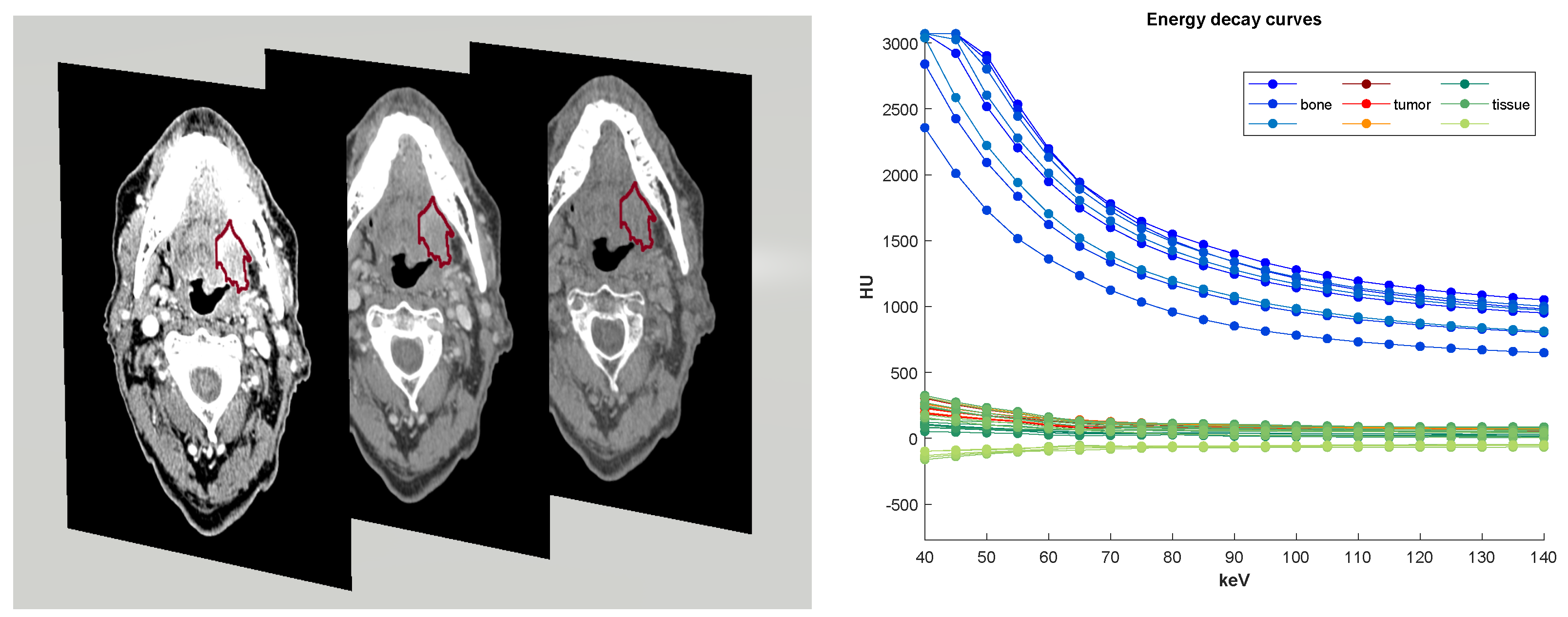
We propose a spatialized mixture of functional regressions model, adapted to the given type of image data, for the model-based clustering of dual-energy CT scans. The images we analyze include spectral curves for each 3D voxel. Each image, denoted Im, is represented as a sample of n observations, where is the ith voxel 3D spatial coordinates.The ith voxel is represented by the curve composed of HU attenuation values measured at energy levels (covariates) , with m being the number of energy levels.
To accommodate the spatial organization of the image together with the functional nature of each of its voxels, we propose spatialized conditional extensions of the general family of model (
1), in which we model the
ith voxel observation of the image using the conditional density
that relates the attenuation curve levels
, given the associated energy levels
, and spatial location
via a convex combination of (non-)linear (semi-)parametric functional regressors
with spatial weights
, that is,
To this purpose, we consider two different spatial constructions of the mixing weights (gating functions) : (i) softmax gates; and (ii) normalized Gaussian gates. The latter is an appropriate choice if more approximation quality is needed, and facilitates the computations in the learning process. We also consider different families to model the functional regressors, including spline and B-spline regression functions that enjoy better curve approximation capabilities, compared to linear or polynomial regression functions.
3.2.1. Functional Regression Components
We have a 3D image volume over a range of energy levels that provide, for each voxel i, an attenuation curve which represents energy-dependent changes in attenuation, which enables a better characterization of the tissue at voxel i. We therefore model the component densities as functional regression models constructed upon the attenuation curves as functional observations. This allows us to accommodate the spectral curve nature of the data. More specifically, in the case of univariate energy levels, we use smooth functional approximations to model, for the ith voxel, the mean spectral curve of the kth component , that is, using polynomial or (B)-spline functions, whose coefficients are .
The conditional density model for each regression is then modeled as a functional Gaussian regressor defined by
, with
being the function approximation onto polynomial or (B-)spline bases
, and the matrix form of the functional regression model is then given by
where
is the unknown parameter vector of regression
k.
3.2.2. Spatial Gating Functions
The constructed functional mixture of regressions model (
5) specifically integrates the spatial constraints in the mixture weights
via functions of the spatial locations
parametrized by vectors of coefficients
. We investigate two choices to this end. The first proposed model is a spatial softmax-gated functional mixture of regression and is defined by (
5) with a softmax gating function:
where
is the unknown parameter vector of the gating functions. We will refer to this model, defined by (
5)–(
7), as the spatial softmax-gated mixture of functional regressions, abbreviated as
SsMFR. The softmax modeling of the mixture weights is a standard choice known in the mixtures-of-experts community. However, its optimization performed at the M step of the EM algorithm, is not analytic and requires numerical Newton–Raphson optimization. This can become costly, especially in larger image applications, such as the one we address.
In the second proposed model, we use a spatial Gaussian-gated functional mixture of regressions, defined by (
5) with a Gaussian-gated function:
in which
are non-negative weights that sum to one,
is the density function of a multivariate Gaussian vector of dimension
d with mean
and covariance matrix
, and
is the parameter vector of the gating functions with
.
We will refer to this model, defined by (
5), (
6) and (
8), as the spatial Gaussian-gated mixture of functional regressions, abbreviated as
SgMFR. This Gaussian gating function was introduced in [
42] to bypass the need for an additional numerical optimization in the inner loop of the EM algorithm. We obtain a closed form updating formula at the M-Step, that is detailed in the next section presenting the derived EM algorithm.
3.2.3. MLE of the SgMFR Model via the EM Algorithm
Based on Equations (
5), (
6) and (
8), the SgMFR joint density
is then derived and the joint log-likelihood we maximize via EM is
The complete-data log-likelihood, upon which the EM algorithm is constructed, is
where
is an indicator variable such that
if
(i.e., if the
ith pair
is generated from the
kth regression component) and
, otherwise. The EM algorithm, after starting with an initial solution
, alternates between the E and M steps until convergence (when there is no longer a significant change in the log-likelihood).
The E-step: Compute the conditional expectation of the complete-data log-likelihood (
10), given the image
and the current estimate
:
where
given by
is the posterior probability that the observed pair
is generated by the
kth regressor. This step therefore only requires the computation of the posterior component membership probabilities
, for
.
The M-step: Calculate the parameter vector update
by maximizing the
Q-function (
11), i.e.,
. By decomposing the
function as
with
and
, the maximization can then be performed by
K separate maximizations with respect to the parameters of the gating and the regression functions.
Updating the gating functions parameters: Maximizing (
13) with respect to
’s corresponds to the M step of a Gaussian mixture model [
32]. The closed-form expressions for updating the parameters are given by
Updating the regression functions parameters: Maximizing (
13) with respect to
corresponds to the M step of standard mixtures of experts with univariate Gaussian regressions. The closed-form updating formulas are given by
3.3. Alternative Two-Fold Approaches
We also investigate an alternative approach to the one derived before, which consists of a two-fold approach, rather than a simultaneous functional approximation and model estimation for segmentation. We first construct approximations of the functional data onto polynomial or (B-)splines bases
via MLE (ordinary least squares in this case) to obtain
Then, we model the density of the resulting coefficient vectors
, which is regarded as the
ith curve representative, by a mixture density with spatial weights of the form
where
and
are the mean and the covariance matrix of each component. The spatial weights
are normalized Gaussians as in (
8) or softmax as in (
7). We will refer to these methods as spatial Gaussian-gated (resp. softmax-gated) mixtures of vectorized functional regressions,
SgMVFR (resp.
SsMVFR).
The EM algorithm for fitting this mixture of spatial mixtures, constructed upon pre-computed polynomial or (B-)spline coefficients with its two variants for modeling the spatial weights, takes a similar form to the previously presented algorithm, and is summarized as follows. The conditional memberships of the E step are given for the softmax-gated model by
and for the Gaussian-gated model by
The latter has the same advantage as explained above. In the M step, the gating functions parameter updates are given by (14)–(16) for the Gaussian-gated model, or through a Newton–Raphson optimization algorithm for the softmax-gated model. The component parameter updates are those of classical multivariate Gaussian mixtures
In a nutshell, to compute a clustering of the image, the label of voxel
i, given the fitted parameters
, is calculated by the Bayes’ allocation rule (
3), in which
is the spatial coordinates of voxel
i with either its direct spectral curve representative
or its pre-calculated functional approximation coefficients
given by (
19).
Appendix A contains the pseudo-codes summarizing the proposed method.
3.4. Time Complexity of the Proposed Algorithms
In this subsection we investigate the time complexity of the proposed algorithms. The time complexity of the E-step of the proposed EM algorithms for the SgMFR and the SsMFR models is of , with n being the number of voxels, m the number of energy levels, d is the number of spatial coordinates (2 or 3), p the number of the number of regression coefficients, and K the number of clusters. For the M step, the SgMFR and the SgMVFR have closed-form updates; The SgMFR requires the calculation of the regression coefficients via weighted least squares with a complexity of . The SgMVFR models require the calculations of the Gaussian means and covariance matrices as in multivariate Gaussian mixtures, and have a complexity of . However, the SsMFR and SsMVFR algorithms require at each iteration inside the M step of the EM algorithm an IRLS loop and the inversion of the Hessian matrix which is of dimension . Therefore, the complexity of the IRLS is approximately of , where IRLS is the average number of iterations required by the internal IRLS algorithm. The complexity here can therefore be an issue for a large number of clusters, and the SgMFR and SgMVFR algorithms can be preferred.
4. Experimental Study
In this section, we describe the evaluation of different versions of our method: mixtures of B-spline and polynomial functional regressions with spatial Gaussian gates (resp. SgMFR-Bspl and SgMFR-poly), mixture of B-spline regressions with softmax gates (SsMFR-Bspl), and mixture of vectorized B-spline regressions with Gaussian gates (SgMVFR-Bspl).
4.1. Data
In total, 91 head and neck DECT scans were evaluated, consisting of HNSCC tumors of different sizes and stages from different primary sites. In our dataset, 34% of tumors are located in the oral cavity, 26% in the oropharynx, 21% in the larynx, 8% in the hypopharynx and 11% in other locations. The tumors’ T-stage [
43] ranges from T1 to T4. Of the patients, 75% were coming for a first diagnostic while 25% were recurrent patients. Institutional review board approval was obtained for this study with a waiver of informed consent. Tumors were contoured by an expert head and neck radiologist. All scans were acquired using a fast kVp switching DECT scanner (GE Healthcare) after administration of IV contrast and reconstructed into 1.25 mm sections of axial slices with a resolution of 0.61 mm, as previously described [
11]. Multienergy VMIs were reconstructed at energy levels from 40 to 140 keV in 5 keV increments at the GE Advantage workstation (4.6; GE Healthcare).
In each DECT scan, we crop volumes of interest (VOIs) of size 150*150*6 containing a tumor, along with the 21-point-spectral curve associated to each selected voxel, in order to reduce the computational demands for an exploratory study, and to exclude regions containing a majority of air voxels around the body. A pre-processing step is also applied to mask any remaining air voxels in the VOI to focus the clustering on tissues.
4.2. Regularization Parameter
In our study, we augmented the statistical estimator in Equation (16) of the covariance matrix of the spatial coordinates within cluster
k, with a regularization parameter
, which controls the amount of spatial dispersion (neighborhood) taken into account in the spatial mixture weights, by
By doing so, we can numerically control the amount of data within cluster k (i.e., its volume). Indeed, if we decompose where is the eigenvectors matrix, and is a diagonal matrix whose diagonal elements are the eigenvalues in decreasing order, then is the volume of cluster k. Since the tumor cluster has in general no strong spatial dispersion, then in practice, we take small values of order .
4.3. Parameter Initialization
For the sake of reproducibility, we start by initializing the regression mixture and weight parameters of the EM algorithm with a coarse clustering solution given by a Voronoi diagram. We build up Voronoi tiles over the selected voxels in the VOI (a square region where air voxels are deleted) with the k-means algorithm applied only on spatial coordinates. Then to fix the number of clusters
K, and to fix the spatio-spectral hyper-parameter
, we assess on a small training set (10 patients) the three metrics described in
Section 4.5. In our experiments,
K is taken to be large enough, say 20, 30 or 40, so that we do not have to perform a full grid search which could be computationally demanding, and the value
around
works very well. The process is run similarly for both methods of mixtures of functional regressions and mixtures of vectorized functional regressions. The range of search values is adapted for each method, and 5 search values are taken in each range. In the end, we use the mean of optimal values over the patients in the train set.
4.4. Baselines
We compare the quantitative and qualitative performance of our methodology with three baseline algorithms. First, we implement a Gaussian mixture model (GMM) with the iterative EM algorithm, using the standard non-reshaped algorithm [
32] to cluster the spectral curves, thus leading to not include spatial coordinates. Because several clusters can become empty through the optimization, we fix an initial number of clusters (
) that ends up providing, on average, the same resulting number of clusters for our method (i.e.,
). Second, we implement k-means clustering, using all vector information available, that is, the input vector is built with spectral information (i.e., the energy decay curve points) concatenated to a vector of spatial information (i.e., the 3D coordinates). The number of clusters is picked to be also
, the number of clusters being stable throughout the optimization. We use the Matlab k-means implementation for images with a reproducible initialization through the built-in ‘imsegkmeans’ function. Third and last, we implement selective search, a machine learning graph-based segmentation method for object recognition. Using a region merging hierarchical approach with an SVM classifier to select the hierarchical rank of the resulting regions, the authors published an open-source code [
44]. We apply selective search on low-, intermediate- and high-energy levels (resp. 40, 65 and 140 keV). These energy levels are used instead of the three RGB image channels. We note that selective search does not predetermine the number of clusters, but specifies a cluster minimum size or favors smaller or larger cluster sizes.
4.5. Metrics
Our clustering methods, as well as the baseline clustering algorithms, are all evaluated using the following three metrics:
A cluster separation index, Davies–Bouldin index (DB), computed on spatial content and on spectral content.
A clustering separation index focused only on the relationship between tumor clusters and other clusters, Davies–Bouldin index on tumor (DB), an adaptation of DB, computed on spatial and on spectral content.
A segmentation score computed on tumor clusters versus ground truth region, the Dice similarity score, that can be computed only on spatial content.
To define tumor clusters, we select the cluster(s) which best cover the tumor, i.e., the ones that give the best Dice score when merged together. Several clusters segmenting the tumor area can indeed represent different tumor subparts, but we only know the tumor primary site contour as the ground truth.
When
C is the ensemble of clusters,
is the Euclidean distance operator,
is the centroid of cluster
, the Davies–Bouldin index is defined as
where
The ‘tumor’ Davies–Bouldin index is adapted as
where
is the region of the merged tumor clusters. The Dice score is defined as
where
is the ground truth region. We summarize the distribution of these index values across the population by computing the mean, median and interquartile range.
5. Results
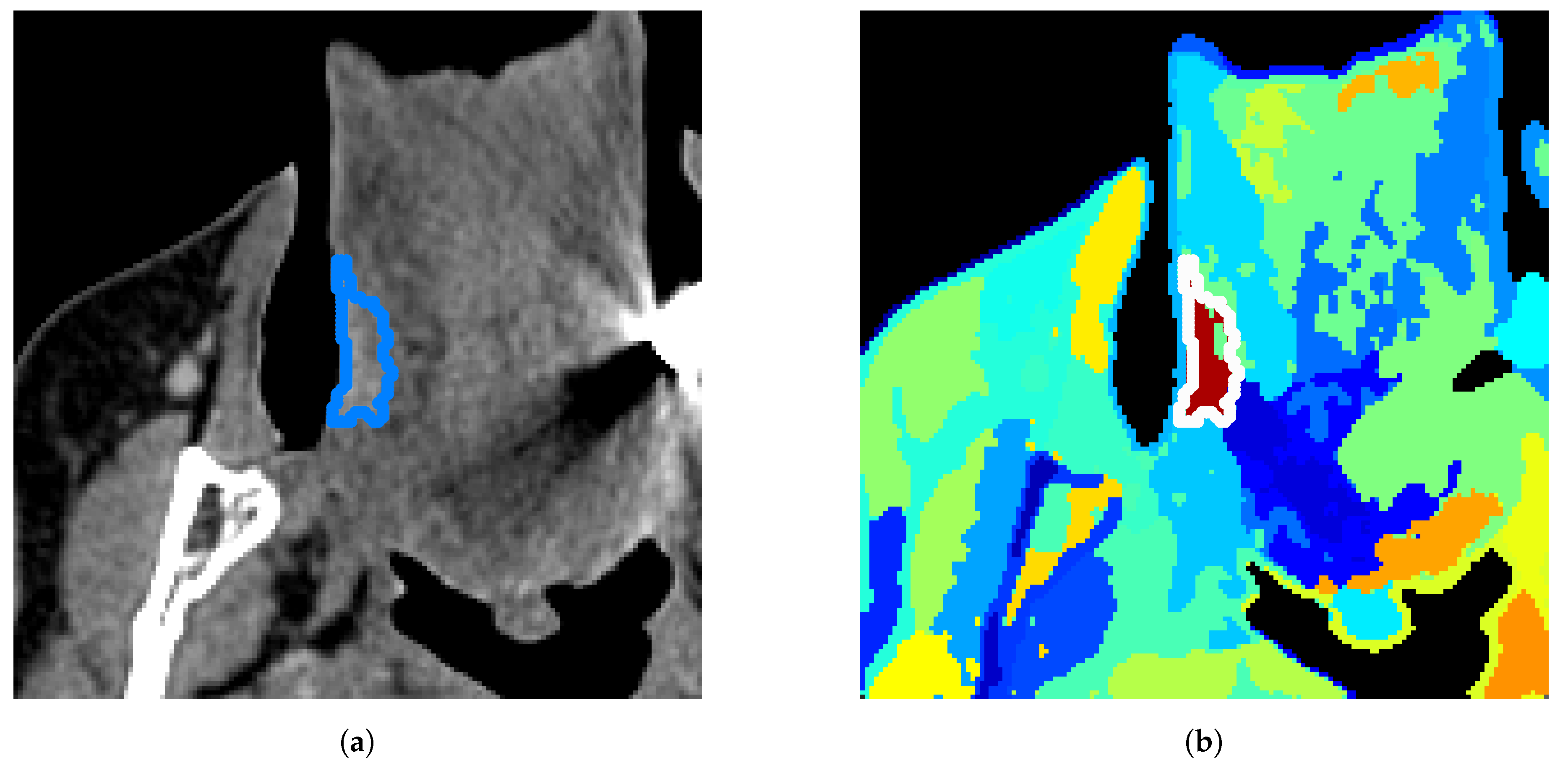
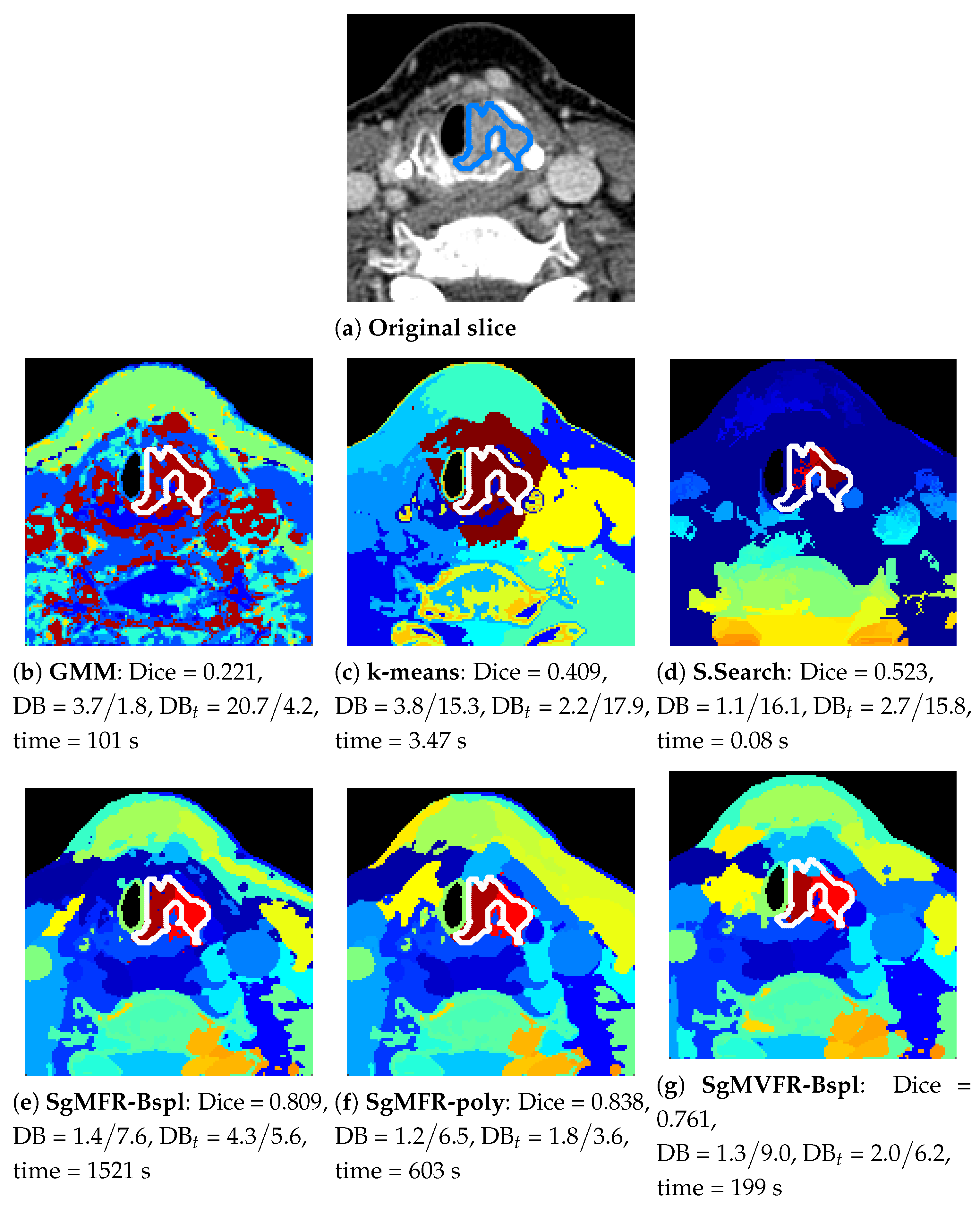
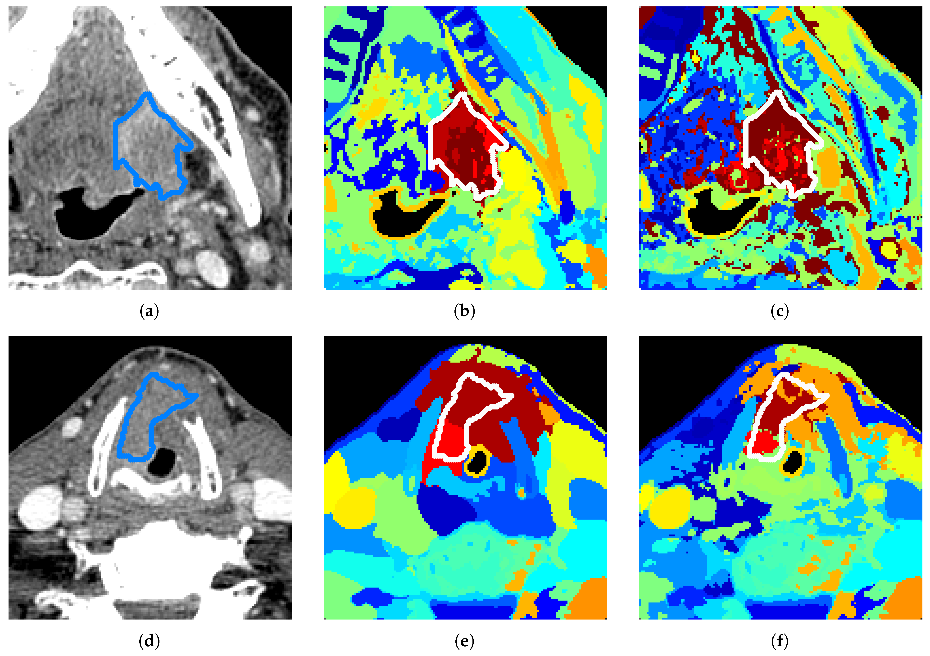
Figure 2 shows an overview of our results for one tumor example. We visualize the results on a 2D slice when the model has been run on the 3D VOI containing this slice.
The top row shows the performance of the baseline algorithms, whereas the bottom row shows our proposed methods. While the baseline approaches attribute a high number of clusters to bone regions containing big spectral variations and miss smaller variations in tissue regions, our methods with Gaussian gates in
Figure 2e–g are able to adapt to relative variations and split the image with more spatial coherence. The results also demonstrate that our method is able to capture tissue characteristics invisible in
Figure 2b–d,h. Note that DB and DB
scores depend on the number of clusters and SsMFR in
Figure 2h has a very low number of clusters (softmax having vanishing clusters in the optimization). GMM and selective search in
Figure 2b,d have around 40 clusters (varying number as explained in
Section 4.4). The results in
Figure 2c,e–g were obtained with 40 clusters.
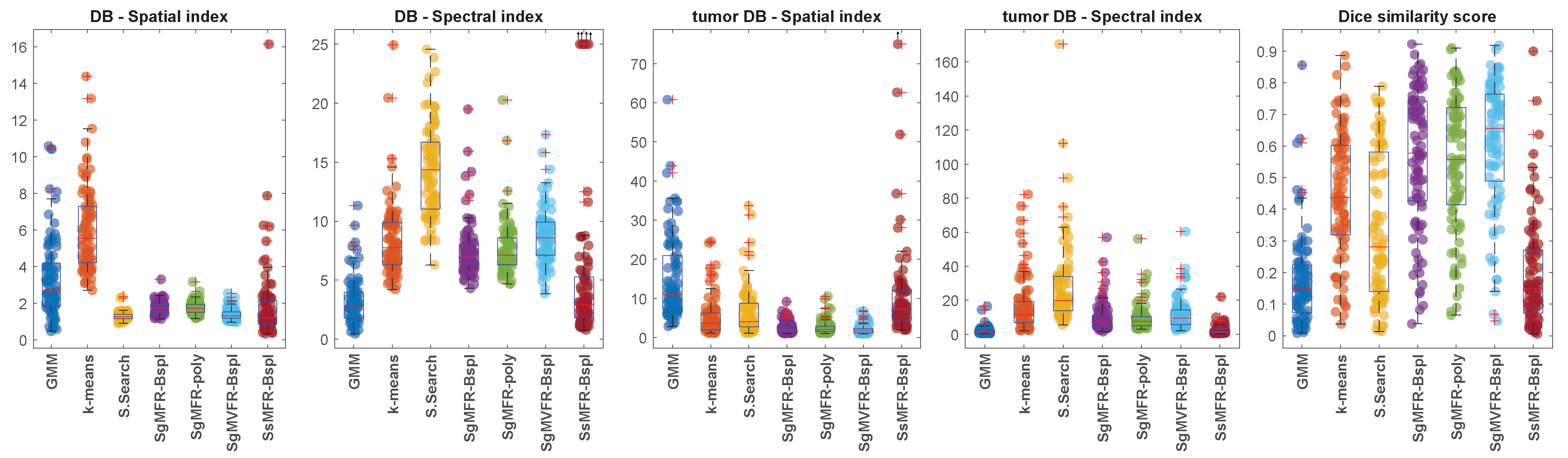
Table 1 and
Figure 3 present the quantitative results obtained with the three clustering metrics defined in
Section 4.5. Among the three proposed methods that outperform the baseline methods in terms of Dice score (SgMFR-Bspl, SgMFR-poly, and SgMVFR-Bspl), we compared the Dice score distribution obtained with SgMFR-poly (which has the lowest median Dice score among the three) to that obtained with the k-means-like baseline (which has the highest median Dice score) with a two-sample
t-test, obtaining
p = 0.0014.
Figure 4 showcases the clustering results obtained when varying the tuning of
. Here, we understand that a smaller
gives a higher preference to the spatial information: clusters are compact and define well-separated areas. On the other hand, a larger
gives a higher priority to the spectral information: clusters more closely match tissue characteristics, but one cluster can be split into tiny voxel groups spread all over the image. The ideal
choice would be a
that prioritizes spectral information, but still achieves some cluster spatial compactness. We assess this through metrics calculated on spectral and spatial content as explained in
Section 4.5. The general tuning of
is determined to be, on average, the optimal hyper-parameter. However, we can see strong improvements in tumor separation, on a case by case basis, with small variation of
. As shown in
Figure 4e,f, the Dice score increases from 0.36 to 0.64. This shows an example out of several results belonging to the lower quartile in the boxplot of Dice scores in
Figure 3 that could be highly improved simply with a specific tuning. Some other examples of results in the lower quartile could be due to small tumors (size inferior to 1cm), although half of these small tumors are actually well-separated with our method, reaching a Dice score as high as 0.84 in the best case (see in
Figure 5).
The proposed algorithms clearly outperform the investigated standard clustering algorithms in terms of the considered metrics, such as the Dice score. In particular, the two approaches based on Gaussian-gating mixture weights, whenever they are directly built upon a functional mixture model (SgMFR), or used with a prior functional data representation of the energy curves (SgMVFR), enjoy both high segmentation capabilities while being computationally effective. The two proposed alternative approaches based on the use of softmax-gating mixture weights (SsMFR and SsMVFR), can, however, be computationally expensive, given that they use, at each EM iteration, a Newton–Raphson optimization; they may lead in some situations to less precise segmentation, typically due to a numerical convergence issue, as compared to the proposed Gaussian-gating-based approaches. As a result, we can suggest to the interested users prioritize the use of the SgMFR and SgMVF approaches when investigating our proposed techniques for DECT clustering. This being said, in order to investigate the statistical significance of the differences in the results of the proposed family of algorithms, it is interesting to perform a statistical study with appropriate statistical testing.
6. Discussion and Conclusions
In this paper, we developed a statistical methodology to cluster intensity attenuation curves in DECT scans. We applied our proposed methods, together with other alternative clustering algorithms used as baselines, to a set of 91 DECT scans of HNSCC tumors. The classical manner of evaluating algorithms for clustering/segmentation is via measures of overlap (such as the Dice score) with a ground truth segmentation. However, as mentioned in the Introduction above, the manual segmentations of HNSCC tumors that are used as “ground truth” can suffer from large inter-rater variability, and do not incorporate in any systematic manner regions immediately adjacent to the tumor that may be biologically important for determining the course of evolution of the tumor. Because of this inherent uncertainty in the appropriate contours of an HNSCC tumor, the main objective in our paper was to compare our clustering results to the manual contouring, but also to explore associations between voxels within the ground truth tumor contour and voxels in the surrounding tissue areas.
Compared to the baseline algorithms, it is clear both visually and quantitatively that our methods using Gaussian gates (SgM(V)FR) produce results that match better the manual segmentation contours. Our method using softmax gates (SsMFR) is less flexible compared to the one with Gaussian gating functions, and thus sometimes leads to non-satisfactory results. Although in terms of qualitative assessment, clusters of SsMFR-Bspl are indeed more spatially compact, quantitative performance in some situations stays similar to GMM baseline. Thus, this variant of the algorithm does not appear to perform well in practice. Using Gaussian gates, however, Dice score distributions are significantly better than the k-means-like algorithm, the best of our baseline methods.
That being said, it is also clear that with Dice scores ranging from nearly 0 to nearly 1, our proposed methods do not recover the “ground truth” segmentations in a reliable and consistent manner. Several reasons may explain this finding. First, our clinical dataset of DECT scans is not uniform, i.e., it includes tumors of highly variable characteristics, in highly variable sizes, locations and environments, which makes it particularly challenging. Moreover, as seen in
Figure 4, changes in parameter tuning can lead to substantial improvement in Dice scores for some tumors. Finally, because of their intricate morphology and often small sizes, HNSCC tumors are inherently difficult to segment. In a recent international challenge, Dice scores of head and neck tumor segmentation ranged across different competition entries between 0.56 and 0.76 [
45].
Most importantly, as argued throughout this paper, the clinical value of recovering the manual segmentations of HNSCC tumors as an objective criterion for evaluating the algorithm is also not clear. In fact, it was recently argued in the clinical literature that AI methods in medical imaging would be more meaningful if evaluated against clinical outcomes, as opposed to an evaluation against radiologists’ performance, due to inherent subjectivity and variability of the latter [
46]. For all the reasons, the objective of this paper was moved away from reproducing the manual contours produced by the radiologist, and was focused instead on developing tools that discover patterns of association in the DECT data.
Our study has several limitations. As discussed above, in our view, the appropriate way of evaluating the methodology’s clinical utility is not by computing Dice scores relative to manually drawn contours. Rather, a more clinically informative evaluation would determine the performance of the recovered clusters in predicting clinical outcome in a machine learning setting, compared to the same predictive algorithm applied with the manual tumor segmentations. Such an evaluation is missing from the present paper; it will be part of a subsequent paper in future work. Another limitation stems from the lack of an automated identification of those clusters that are associated with the tumor region. Right now, we choose those clusters that maximize overlap with the manually segmented tumor region. Ideally, however, the abnormal tumor clusters should be identified automatically, by selecting those clusters that have the highest association with clinical outcomes. In this manner, the automated cluster identification can be naturally made part of a single machine learning pipeline for predicting clinical outcomes. Yet another limitation comes from the very small size of the subset of tumors (n = 10) over which we estimated the algorithm parameters ( and number of clusters), before applying the algorithm to the remaining 81 tumors in our dataset. A larger dataset, together with additional patient-specific tuning will help tune the algorithm’s performance.
The need for the improvements described above is clear, and they will be made part of a subsequent publication. In the present article, we chose to focus on the theoretical and algorithmic developments. As mentioned in the Introduction, this is the first time to our knowledge that statistical tools from the functional data analysis field are put into practice with DECT data. As such, the present paper remains an inherently exploratory one in its experimental framework.
Nevertheless, we believe that we provide several important technical and methodological contributions. We constructed a functional regression mixture model that integrates spatial content into the mixture weights, and we developed a dedicated EM algorithm to estimate the optimal model parameters. Our mixture-based model is a highly flexible statistical approach allowing for many choices of the parametric form of the component densities. We proposed two candidate designs for the mixture weights, normalized Gaussian gates and softmax gates. The Gaussian-gate closed-form solution for spatial mixture weight updates considerably reduces the computation time while also providing solutions with better clustering index values, compared to the Newton–Raphson optimization algorithm needed at each update of the softmax-gating parameters.


