
Validation and Optimization of Proximal Femurs Microstructure Analysis Using High Field and Ultra-High Field MRI

 ,
, 

Abstract
:1. Introduction
2. Materials and Methods
2.1. Sample Preparation
2.2. Imaging
2.2.1. µCT Imaging
2.2.2. MRI Imaging
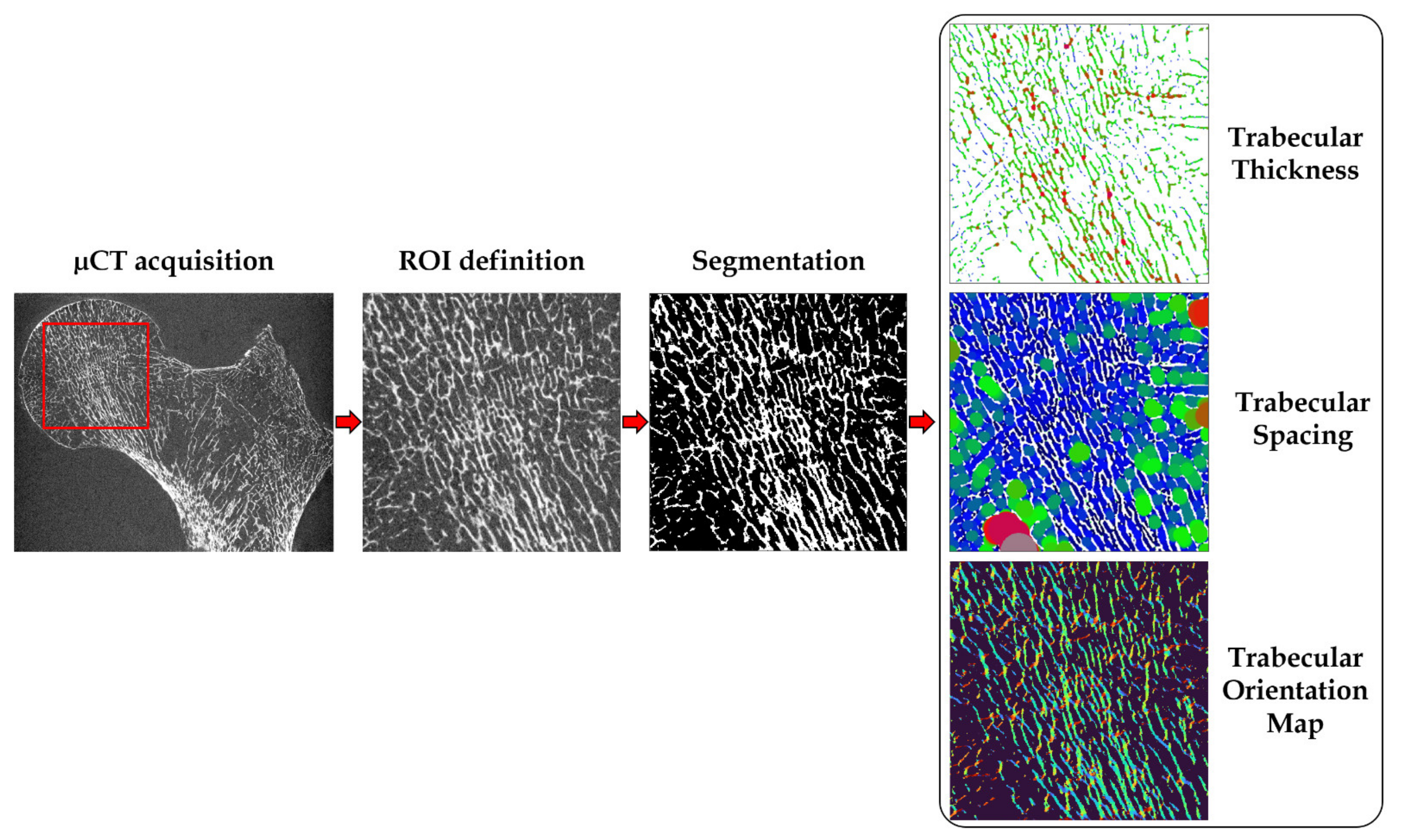
2.3. Image Analysis
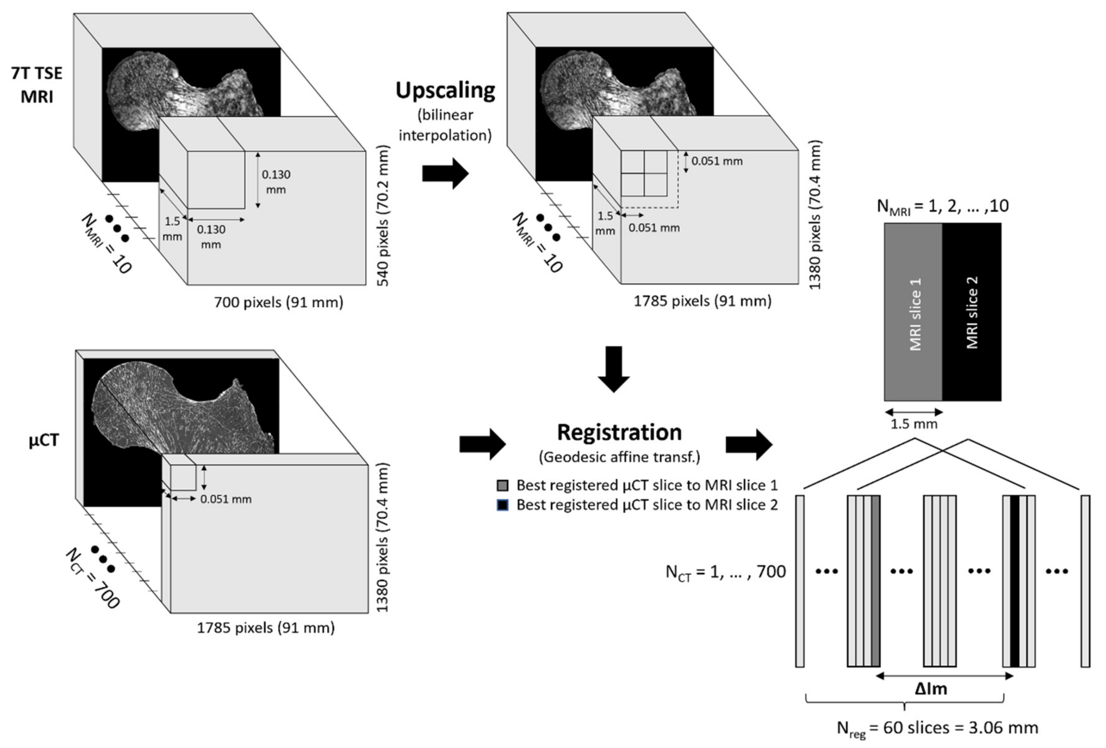
2.3.1. Image Registration
2.3.2. Bone Morphological Quantification
2.3.3. Bone Mineral Density Assessment
2.4. Mechanical Testing
3. Results
3.1. Registration Quality
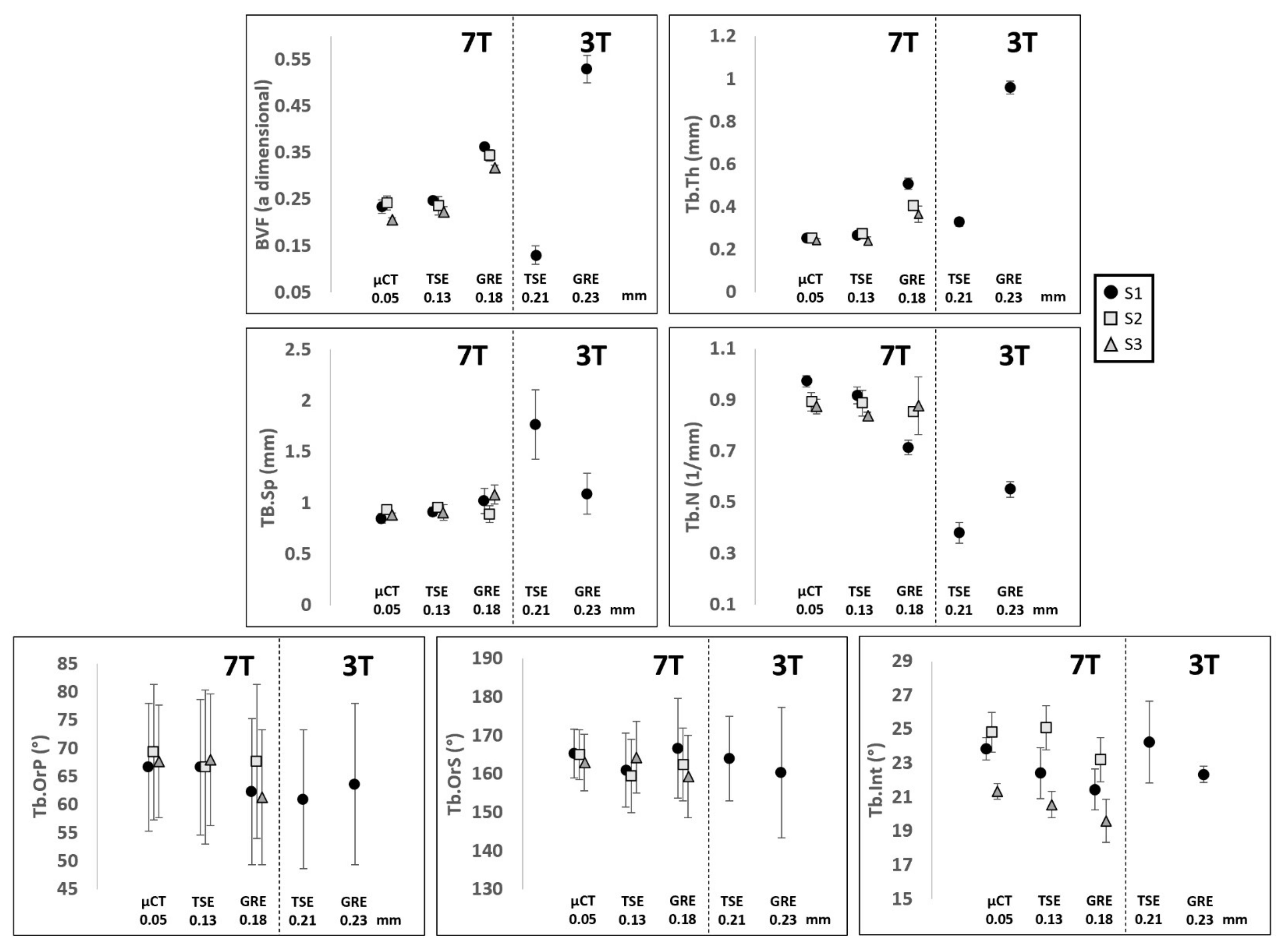
3.2. Selection of the Optimal MRI Sequence
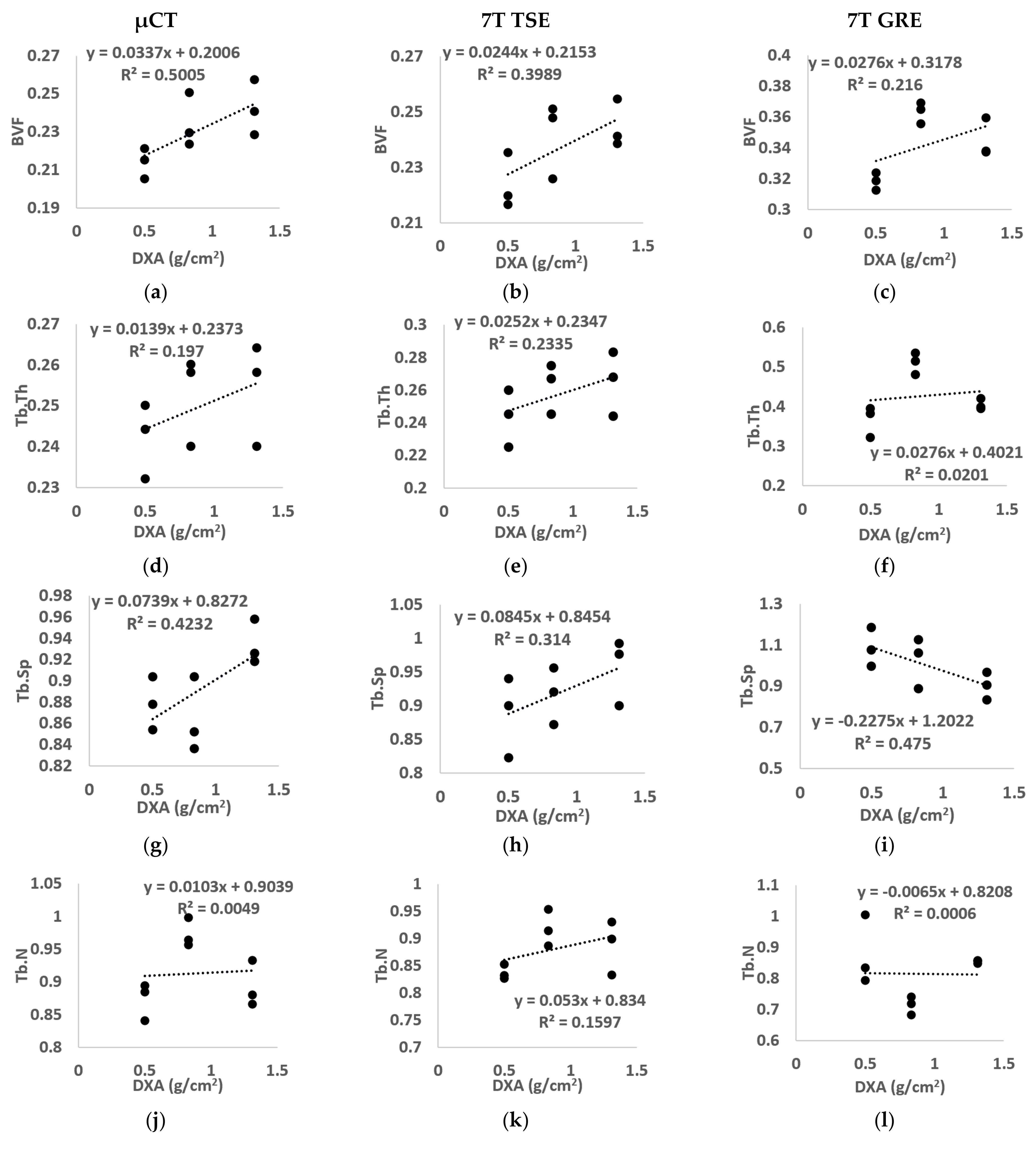
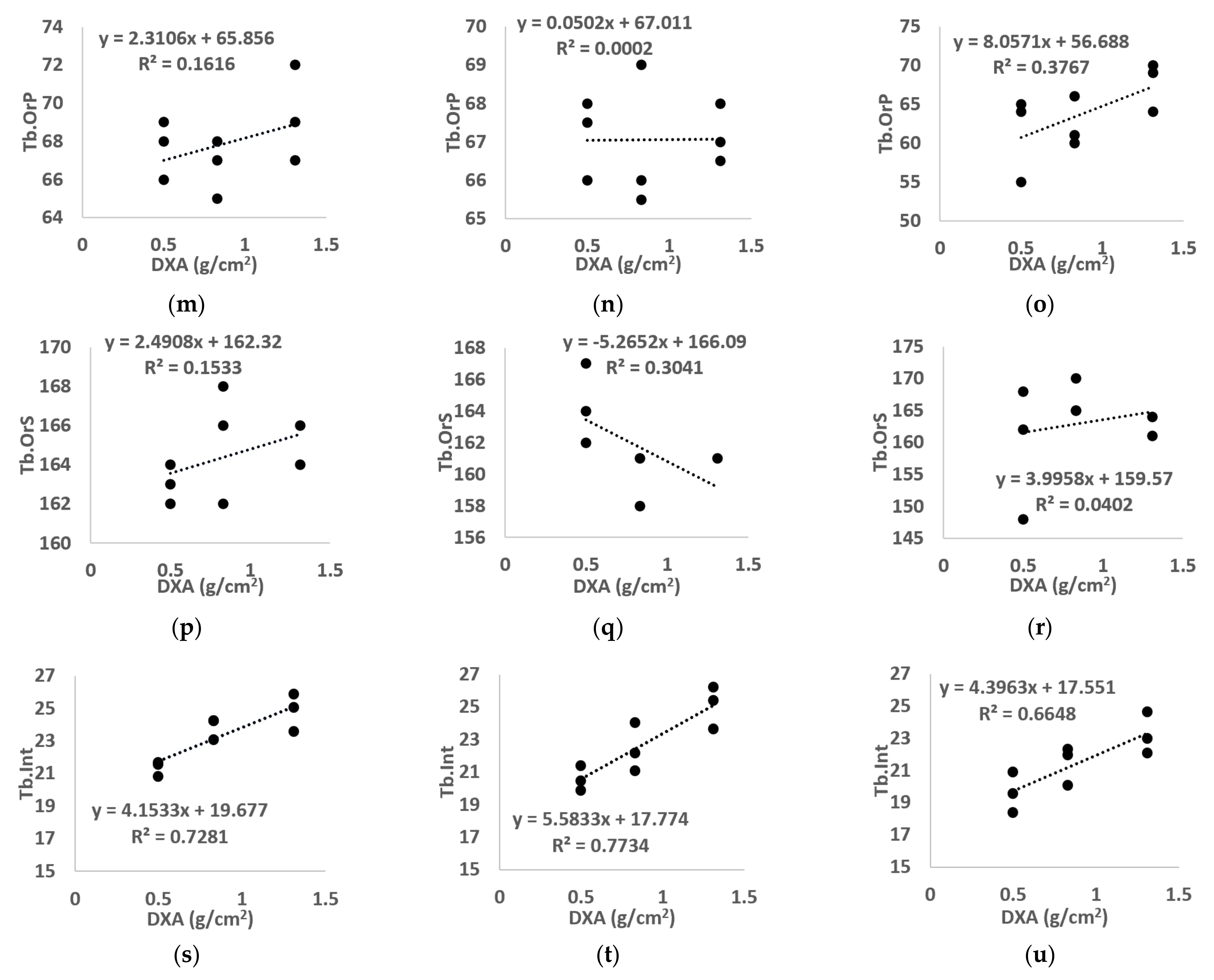
3.3. Correlation between DXA-BMD and Microarchitecture
3.4. Correlation between DXA-BMD and Both μCT- and MR- Derived BMD
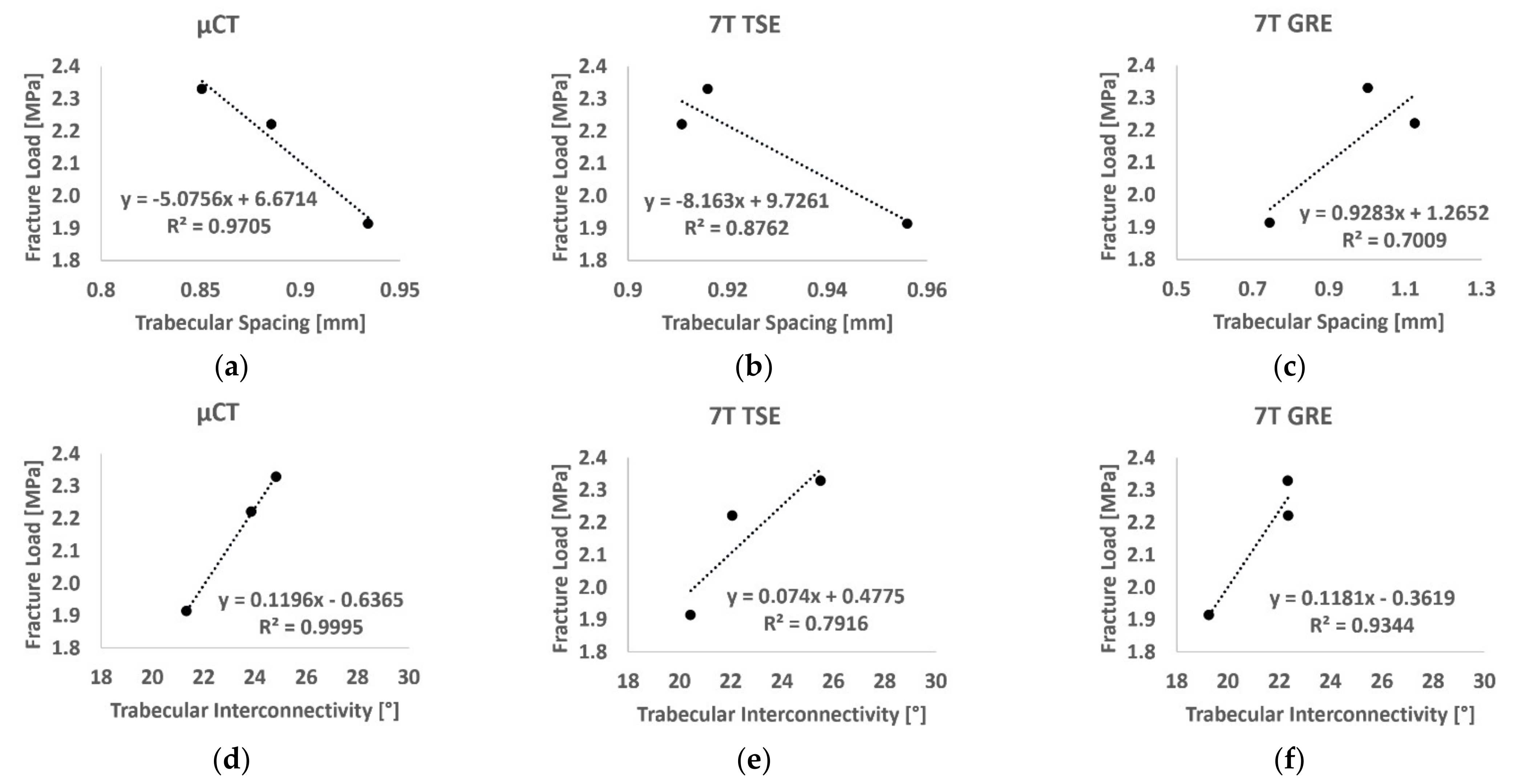
3.5. Correlation between Failure Load and Bone Morphology
4. Discussion
5. Conclusions
Author Contributions
Funding
Institutional Review Board Statement
Informed Consent Statement
Data Availability Statement
Conflicts of Interest
References
- Chang, G.; Rajapakse, C.S.; Chen, C.; Welbeck, A.; Egol, K.; Regatte, R.R.; Saha, P.K.; Honig, S. 3-T MR Imaging of Proximal Femur Microarchitecture in Subjects with and without Fragility Fracture and Nonosteoporotic Proximal Femur Bone Mineral Density. Radiology 2018, 287, 608–619. [Google Scholar] [CrossRef] [Green Version]
- Hernlund, E.; Svedbom, A.; Ivergård, M.; Compston, J.; Cooper, C.; Stenmark, J.; McCloskey, E.V.; Jönsson, B.; Kanis, J.A. Osteoporosis in the European Union: Medical Management, Epidemiology and Economic Burden: A Report Prepared in Collaboration with the International Osteoporosis Foundation (IOF) and the European Federation of Pharmaceutical Industry Associations (EFPIA). Arch. Osteoporos. 2013, 8, 136. [Google Scholar] [CrossRef] [Green Version]
- Schuit, S.C.E.; van der Klift, M.; Weel, A.E.A.M.; de Laet, C.E.D.H.; Burger, H.; Seeman, E.; Hofman, A.; Uitterlinden, A.G.; van Leeuwen, J.P.T.M.; Pols, H.A.P. Fracture Incidence and Association with Bone Mineral Density in Elderly Men and Women: The Rotterdam Study. Bone 2004, 34, 195–202. [Google Scholar] [CrossRef]
- Nayak, S.; Edwards, D.L.; Saleh, A.A.; Greenspan, S.L. Systematic Review and Meta-Analysis of the Performance of Clinical Risk Assessment Instruments for Screening for Osteoporosis or Low Bone Density. Osteoporos. Int. 2015, 26, 1543–1554. [Google Scholar] [CrossRef] [PubMed]
- Humadi, A.; Alhadithi, R.; Alkudiari, S. Validity of the DEXA Diagnosis of Involutional Osteoporosis in Patients with Femoral Neck Fractures. Indian J. Orthop. 2010, 44, 73. [Google Scholar] [CrossRef] [PubMed]
- Soldati, E.; Rossi, F.; Vicente, J.; Guenoun, D.; Pithioux, M.; Iotti, S.; Malucelli, E.; Bendahan, D. Survey of MRI Usefulness for the Clinical Assessment of Bone Microstructure. Int. J. Mol. Sci. 2021, 22, 2509. [Google Scholar] [CrossRef]
- Lam, D.; Wootton-Gorges, S.L.; McGahan, J.P.; Stern, R.; Boone, J.M. Abdominal Pediatric Cancer Surveillance Using Serial Computed Tomography: Evaluation of Organ Absorbed Dose and Effective Dose. Semin. Oncol. 2011, 38, 128–135. [Google Scholar] [CrossRef] [Green Version]
- Damilakis, J.; Adams, J.E.; Guglielmi, G.; Link, T.M. Radiation Exposure in X-Ray-Based Imaging Techniques Used in Osteoporosis. Eur. Radiol. 2010, 20, 2707–2714. [Google Scholar] [CrossRef] [PubMed] [Green Version]
- Guenoun, D.; Pithioux, M.; Souplet, J.-C.; Guis, S.; Le Corroller, T.; Fouré, A.; Pauly, V.; Mattei, J.-P.; Bernard, M.; Guye, M.; et al. Assessment of Proximal Femur Microarchitecture Using Ultra-High Field MRI at 7 Tesla. Diagn. Interv. Imaging 2020, 101, 45–53. [Google Scholar] [CrossRef]
- Chang, G.; Boone, S.; Martel, D.; Rajapakse, C.S.; Hallyburton, R.S.; Valko, M.; Honig, S.; Regatte, R.R. MRI Assessment of Bone Structure and Microarchitecture: Bone Structure and Microarchitecture. J. Magn. Reson. Imaging 2017, 46, 323–337. [Google Scholar] [CrossRef] [PubMed]
- Krug, R.; Carballido-Gamio, J.; Banerjee, S.; Burghardt, A.J.; Link, T.M.; Majumdar, S. In Vivo Ultra-High-Field Magnetic Resonance Imaging of Trabecular Bone Microarchitecture at 7 T. J. Magn. Reson. Imaging 2008, 27, 854–859. [Google Scholar] [CrossRef] [PubMed]
- Majumdar, S.; Genant, H.K.; Grampp, S.; Newitt, D.C.; Truong, V.-H.; Lin, J.C.; Mathur, A. Correlation of Trabecular Bone Structure with Age, Bone Mineral Density, and Osteoporotic Status: In Vivo Studies in the Distal Radius Using High Resolution Magnetic Resonance Imaging. J. Bone Miner. Res. 1997, 12, 111–118. [Google Scholar] [CrossRef] [PubMed]
- Krug, R.; Carballido-Gamio, J.; Burghardt, A.J.; Kazakia, G.; Hyun, B.H.; Jobke, B.; Banerjee, S.; Huber, M.; Link, T.M.; Majumdar, S. Assessment of Trabecular Bone Structure Comparing Magnetic Resonance Imaging at 3 Tesla with High-Resolution Peripheral Quantitative Computed Tomography Ex Vivo and In Vivo. Osteoporos. Int. 2008, 19, 653–661. [Google Scholar] [CrossRef]
- Magland, J.F.; Wald, M.J.; Wehrli, F.W. Spin-Echo Micro-MRI of Trabecular Bone Using Improved 3D Fast Large-Angle Spin-Echo (FLASE). Magn. Reson. Med. 2009, 61, 1114–1121. [Google Scholar] [CrossRef] [Green Version]
- Rajapakse, C.S.; Kobe, E.A.; Batzdorf, A.S.; Hast, M.W.; Wehrli, F.W. Accuracy of MRI-Based Finite Element Assessment of Distal Tibia Compared to Mechanical Testing. Bone 2018, 108, 71–78. [Google Scholar] [CrossRef]
- Chang, G.; Deniz, C.M.; Honig, S.; Rajapakse, C.S.; Egol, K.; Regatte, R.R.; Brown, R. Feasibility of Three-Dimensional MRI of Proximal Femur Microarchitecture at 3 Tesla Using 26 Receive Elements without and with Parallel Imaging: 3D MRI of Proximal Femur Microarchitecture. J. Magn. Reson. Imaging 2014, 40, 229–238. [Google Scholar] [CrossRef] [Green Version]
- Majumdar, S.; Newitt, D.; Mathur, A.; Osman, D.; Gies, A.; Chiu, E.; Lotz, J.; Kinney, J.; Genant, H. Magnetic Resonance Imaging of Trabecular Bone Structure in the Distal Radius: Relationship with X-Ray Tomographic Microscopy and Biomechanics. Osteoporos. Int. 1996, 6, 376–385. [Google Scholar] [CrossRef] [PubMed]
- Tjong, W.; Kazakia, G.J.; Burghardt, A.J.; Majumdar, S. The Effect of Voxel Size on High-Resolution Peripheral Computed Tomography Measurements of Trabecular and Cortical Bone Microstructure: HR-PQCT Voxel Size Effects on Bone Microstructural Measurements. Med. Phys. 2012, 39, 1893–1903. [Google Scholar] [CrossRef] [Green Version]
- Burghardt, A.J.; Link, T.M.; Majumdar, S. High-Resolution Computed Tomography for Clinical Imaging of Bone Microarchitecture. Clin. Orthop. Relat. Res. 2011, 469, 2179–2193. [Google Scholar] [CrossRef] [PubMed] [Green Version]
- Robitaille, P.-M.; Berliner, L. Ultra High. Field Magnetic Resonance Imaging; Springer: Berlin/Heidelberg, Germany, 2006; ISBN 978-0-387-34231-3. [Google Scholar]
- Soldati, E.; Pithioux, M.; Bendahan, D.; Vicente, J. MRI Assessment of Bone Microarchitecture in Human Femurs: The Issue of Air Bubbles Artefacts. In Proceedings of the ISMRM 2020, Virtual Conference & Exibition, 8–14 August 2020. [Google Scholar] [CrossRef]
- RX Solutions SAS. 3D X-ray Tomography Systems; RX Solutions SAS: Chavanod, France, 2006. [Google Scholar]
- Chang, G.; Honig, S.; Brown, R.; Deniz, C.M.; Egol, K.A.; Babb, J.S.; Regatte, R.R.; Rajapakse, C.S. Finite Element Analysis Applied to 3-T MR Imaging of Proximal Femur Microarchitecture: Lower Bone Strength in Patients with Fragility Fractures Compared with Control Subjects. Radiology 2014, 272, 464–474. [Google Scholar] [CrossRef]
- Techawiboonwong, A.; Song, H.K.; Magland, J.F.; Saha, P.K.; Wehrli, F.W. Implications of Pulse Sequence in Structural Imaging of Trabecular Bone. J. Magn. Reson. Imaging 2005, 22, 647–655. [Google Scholar] [CrossRef] [PubMed]
- Hisham, M.B.; Yaakob, S.N.; Raof, R.A.A.; Nazren, A.B.A.; Embedded, N.M.W. Template Matching Using Sum of Squared Difference and Normalized Cross Correlation. In Proceedings of the 2015 IEEE Student Conference on Research and Development (SCOReD), Kuala Lumpur, Malaysia, 13–14 December 2015; pp. 100–104. [Google Scholar]
- Dachena, C.; Casu, S.; Fanti, A.; Lodi, M.B.; Mazzarella, G. Combined Use of MRI, FMRIand Cognitive Data for Alzheimer’s Disease: Preliminary Results. Appl. Sci. 2019, 9, 3156. [Google Scholar] [CrossRef] [Green Version]
- Dougherty, R.; Kunzelmann, K.-H. Computing Local Thickness of 3D Structures with ImageJ. Microsc. Microanal. 2007, 13. [Google Scholar] [CrossRef]
- Brun, E.; Ferrero, C.; Vicente, J. Fast Granulometry Operator for the 3D Identification of Cell Structures. Fundam. Inform. 2017, 155, 363–372. [Google Scholar] [CrossRef]
- Brun, E.; Vicente, J.; Topin, F.; Occelli, R. IMorph: A 3D Morphological Tool to Fully Analyze All Kind of Cellular Materials. CELLMET-Symposium, Dresden, Germany, 22–26 September 2008; Available online: http://imorph.sourceforge.net/Articles/Cellmet2008.pdf.
- Johansson, M.V.; Testa, F.; Perrier, P.; Vicente, J.; Bonnet, J.P.; Moulin, P.; Graur, I. Determination of an Effective Pore Dimension for Microporous Media. Int. J. Heat Mass Transf. 2019, 142, 118412. [Google Scholar] [CrossRef] [Green Version]
- Goodfellow, I.; Bengio, Y.; Courville, A. Deep Learning (Adaptive Computation and Machine Learning Series); The MIT Press: Cambridge, MA, USA, 2016; ISBN 0-262-03561-8. [Google Scholar]
- Koo, T.K.; Li, M.Y. A Guideline of Selecting and Reporting Intraclass Correlation Coefficients for Reliability Research. J. Chiropr. Med. 2016, 15, 155–163. [Google Scholar] [CrossRef] [Green Version]
- Arokoski, M.H.; Arokoski, J.P.A.; Vainio, P.; Niemitukia, L.H.; Kröger, H.; Jurvelin, J.S. Comparison of DXA and MRI Methods for Interpreting Femoral Neck Bone Mineral Density. J. Clin. Densitom. 2002, 5, 289–296. [Google Scholar] [CrossRef]
- Kröger, H.; Vainio, P.; Nieminen, J.; Kotaniemi, A. Comparison of Different Models for Interpreting Bone Mineral Density Measurements Using DXA and MRI Technology. Bone 1995, 17, 157–159. [Google Scholar] [CrossRef]
- Ramponi, D.R.; Kaufmann, J.; Drahnak, G. Hip Fractures. Adv. Emerg. Nurs. J. 2018, 40, 8–15. [Google Scholar] [CrossRef]
- Laval-Jeantet, A.-M.; Bergot, C.; Carroll, R.; Garcia-Schaefer, F. Cortical Bone Senescence and Mineral Bone Density of the Humerus. Calcif. Tissue Int. 1983, 35, 268–272. [Google Scholar] [CrossRef] [PubMed]
- Manske, S.L.; Liu-Ambrose, T.; Cooper, D.M.L.; Kontulainen, S.; Guy, P.; Forster, B.B.; McKay, H.A. Cortical and Trabecular Bone in the Femoral Neck Both Contribute to Proximal Femur Failure Load Prediction. Osteoporos. Int. 2009, 20, 445–453. [Google Scholar] [CrossRef]
- Eckstein, F.; Wunderer, C.; Boehm, H.; Kuhn, V.; Priemel, M.; Link, T.M.; Lochmüller, E.-M. Reproducibility and Side Differences of Mechanical Tests for Determining the Structural Strength of the Proximal Femur. J. Bone Miner. Res. 2003, 19, 379–385. [Google Scholar] [CrossRef] [PubMed]
- Le Corroller, T.; Halgrin, J.; Pithioux, M.; Guenoun, D.; Chabrand, P.; Champsaur, P. Combination of Texture Analysis and Bone Mineral Density Improves the Prediction of Fracture Load in Human Femurs. Osteoporos. Int. 2012, 23, 163–169. [Google Scholar] [CrossRef] [PubMed]
- Seifert, A.C.; Li, C.; Rajapakse, C.S.; Bashoor-Zadeh, M.; Bhagat, Y.A.; Wright, A.C.; Zemel, B.S.; Zavaliangos, A.; Wehrli, F.W. Bone Mineral 31P and Matrix-Bound Water Densities Measured by Solid-State 31P and 1H MRI: Bone Density Quantification by Mri. NMR Biomed. 2014, 27, 739–748. [Google Scholar] [CrossRef] [Green Version]
- Majumdar, S.; Link, T.M.; Augat, P.; Lin, J.C.; Newitt, D.; Lane, N.E.; Genant, H.K. Trabecular Bone Architecture in the Distal Radius Using Magnetic Resonance Imaging in Subjects with Fractures of the Proximal Femur. Osteoporos. Int. 1999, 10, 231–239. [Google Scholar] [CrossRef] [PubMed]
- Krug, R.; Banerjee, S.; Han, E.T.; Newitt, D.C.; Link, T.M.; Majumdar, S. Feasibility of in Vivo Structural Analysis of High-Resolution Magnetic Resonance Images of the Proximal Femur. Osteoporos. Int. 2005, 16, 1307–1314. [Google Scholar] [CrossRef]
- Soldati, E.; Escoffier, L.; Gabriel, S.; Ogier, A.C.; Chagnaud, C.; Mattei, J.P.; Cammilleri, S.; Bendahan, D.; Guis, S. Assessment of in Vivo Bone Microarchitecture Changes in an Anti-TNFα Treated Psoriatic Arthritic Patient. PLoS ONE 2021, 16, e0251788. [Google Scholar] [CrossRef]
- Studholme, C.; Hill, D.L.G.; Hawkes, D.J. Automated Three-Dimensional Registration of Magnetic Resonance and Positron Emission Tomography Brain Images by Multiresolution Optimization of Voxel Similarity Measures. Med. Phys. 1997, 24, 25–35. [Google Scholar] [CrossRef] [PubMed]
- Penney, G.P.; Weese, J.; Little, J.A.; Desmedt, P.; Hill, D.L.G.; Hawkes, D.J. A Comparison of Similarity Measures for Use in 2-D–3-D Medical Image Registration. IEEE Trans. Med. Imaging 1998, 17, 10. [Google Scholar] [CrossRef]
- Andronache, A.; Cattin, P.; Székely, G. Local Intensity Mapping for Hierarchical Non-rigid Registration of Multi-modal Images Using the Cross-Correlation Coefficient. In Biomedical Image Registration; Pluim, J.P.W., Likar, B., Gerritsen, F.A., Eds.; Lecture Notes in Computer Science; Springer: Berlin/Heidelberg, Germany, 2006; Volume 4057, pp. 26–33. ISBN 978-3-540-35648-6. [Google Scholar]
- Zhao, C.; Carass, A.; Jog, A.; Prince, J.L. Effects of Spatial Resolution on Image Registration; Styner, M.A., Angelini, E.D., Eds.; SPIE: San Diego, CA, USA, 2016; p. 97840Y. [Google Scholar]


| Seq. | TR/TE (ms) | Flip Angle (°) | FoV (mm) | Bandwidth (Hz/Px) | NeX | Voxel Size (mm) | Slice Thickness (mm) | Slices | Acq.Time (min:sec) |
|---|---|---|---|---|---|---|---|---|---|
| 7T TSE | 1040/14 | 150 | 97 × 130 | 244 | 2 | 0.13 × 0.13 | 1.5 | 10 | 17:45 |
| 7T GRE | 11/5.60 | 12 | 120 × 175 | 330 | 3 | 0.18 × 0.18 | 1 | 48 | 9:27 |
| 3T TSE | 1170/12 | 140 | 119 × 119 | 255 | 2 | 0.21 × 0.21 | 1.1 | 36 | 16:45 |
| 3T GRE | 16.5/7.78 | 10 | 120 × 120 | 130 | 2 | 0.23 × 0.23 | 1.1 | 40 | 11:17 |
| S1 | 7T TSE—μCT | 7T GRE—μCT | 3T TSE—μCT | 3T GRE—μCT |
|---|---|---|---|---|
| NCC score | 0.93 ± 0.01 | 0.86 ± 0.01 | 0.94 ± 0.01 | 0.75 ± 0.01 |
| ΔIm | 67 ± 7 (59) | 36 ± 13 (39) | 42 ± 16 (43) | 50 ± 18 (43) |
| BVF | Tb.Th | Tb.Sp | Tb.N | Tb.OrP | Tb.OrS | Tb.Int | ||
|---|---|---|---|---|---|---|---|---|
| S1 (BMD-DXA = 0.83 g/cm2) | µCT | 0.23 ± 0.01 | 0.25 ± 0.01 | 0.86 ± 0.04 | 0.97 ± 0.03 | 67 ± 11 | 165 ± 6 | 23.84 ± 0.66 |
| 7T TSE | 0.24 ± 0.01 | 0.26 ± 0.02 | 0.92 ± 0.04 | 0.92 ± 0.03 | 67 ± 13 | 161 ± 10 | 22.41 ± 1.50 | |
| Max diff% | 8% | 6% | 8% | 8% | 1% | 3% | 9% | |
| 7T GRE | 0.36 ± 0.01 | 0.50 ± 0.03 | 1.02 ± 0.03 | 0.71 ± 0.03 | 62 ± 12 | 167 ± 10 | 21.44 ± 1.20 | |
| Max diff% | 63% | 107% | 27% | 32% | 10% | 5% | 13% | |
| S2 (BMD-DXA = 1.31 g/cm2) | µCT | 0.24 ± 0.01 | 0.25 ± 0.01 | 0.93 ± 0.02 | 0.89 ± 0.04 | 69 ± 12 | 165 ± 7 | 24.83 ± 1.18 |
| 7T TSE | 0.24 ± 0.02 | 0.26 ± 0.01 | 0.96 ± 0.05 | 0.89 ± 0.05 | 67 ± 14 | 160 ± 9 | 25.08 ± 1.31 | |
| Max diff% | 10% | 7% | 5% | 7% | 7% | 4% | 5% | |
| 7T GRE | 0.34 ± 0.01 | 0.40 ± 0.02 | 0.89 ± 0.08 | 0.85 ± 0.03 | 68 ± 14 | 162 ± 10 | 23.21 ± 1.29 | |
| Max diff% | 57% | 64% | 13% | 9% | 4% | 3% | 8% | |
| S3 (BMD-DXA = 0.50 g/cm2) | µCT | 0.21 ± 0.01 | 0.24 ± 0.01 | 0.88 ± 0.03 | 0.87 ± 0.03 | 68 ± 10 | 163 ± 7 | 21.33 ± 0.46 |
| 7T TSE | 0.22 ± 0.01 | 0.24 ± 0.02 | 0.89 ± 0.06 | 0.84 ± 0.02 | 68 ± 12 | 164 ± 11 | 20.56 ± 0.77 | |
| Max diff% | 11% | 12% | 5% | 6% | 3% | 2% | 6% | |
| 7T GRE | 0.32 ± 0.01 | 0.37 ± 0.04 | 1.08 ± 0.09 | 0.88 ± 0.11 | 61 ± 12 | 159 ± 9 | 19.60 ± 1.27 | |
| Max diff% | 55% | 70% | 35% | 12% | 17% | 9% | 12% |
Publisher’s Note: MDPI stays neutral with regard to jurisdictional claims in published maps and institutional affiliations. |
© 2021 by the authors. Licensee MDPI, Basel, Switzerland. This article is an open access article distributed under the terms and conditions of the Creative Commons Attribution (CC BY) license (https://creativecommons.org/licenses/by/4.0/).
Share and Cite
Soldati, E.; Vicente, J.; Guenoun, D.; Bendahan, D.; Pithioux, M. Validation and Optimization of Proximal Femurs Microstructure Analysis Using High Field and Ultra-High Field MRI. Diagnostics 2021, 11, 1603. https://doi.org/10.3390/diagnostics11091603
Soldati E, Vicente J, Guenoun D, Bendahan D, Pithioux M. Validation and Optimization of Proximal Femurs Microstructure Analysis Using High Field and Ultra-High Field MRI. Diagnostics. 2021; 11(9):1603. https://doi.org/10.3390/diagnostics11091603
Chicago/Turabian StyleSoldati, Enrico, Jerome Vicente, Daphne Guenoun, David Bendahan, and Martine Pithioux. 2021. "Validation and Optimization of Proximal Femurs Microstructure Analysis Using High Field and Ultra-High Field MRI" Diagnostics 11, no. 9: 1603. https://doi.org/10.3390/diagnostics11091603
APA StyleSoldati, E., Vicente, J., Guenoun, D., Bendahan, D., & Pithioux, M. (2021). Validation and Optimization of Proximal Femurs Microstructure Analysis Using High Field and Ultra-High Field MRI. Diagnostics, 11(9), 1603. https://doi.org/10.3390/diagnostics11091603