
Intelligent Bone Age Assessment: An Automated System to Detect a Bone Growth Problem Using Convolutional Neural Networks with Attention Mechanism

 ,
,  , ,
, , 
Abstract
1. Introduction
2. Computerized Bone Age Assessment
- Integration of the spatial-wise attention mechanism that aims to allocate more weights towards the optimal regions of interest.
- Better distribution of training, validation, and testing data, where they are distributed according to the ratio of 8:1:1, respectively.
- Extensive comparison for the data normalization stage that covers state-of-the-art deep learning architectures for segmentation and point of interest localization.
- A more robust bone age assessment system is produced without utilizing the gender information. This step is taken to support patient’s privacy issues where some of them are reluctant to disclose their gender information.
3. Related Works
4. Methods
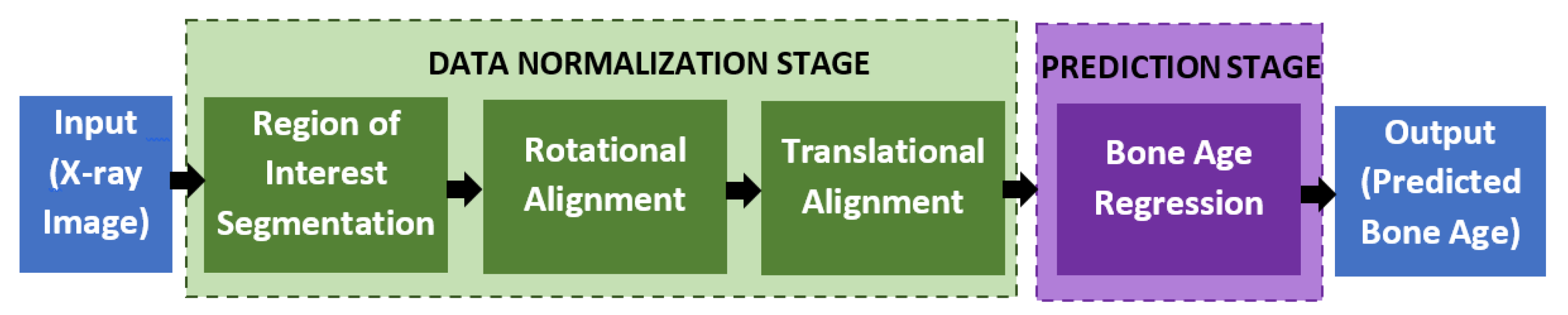
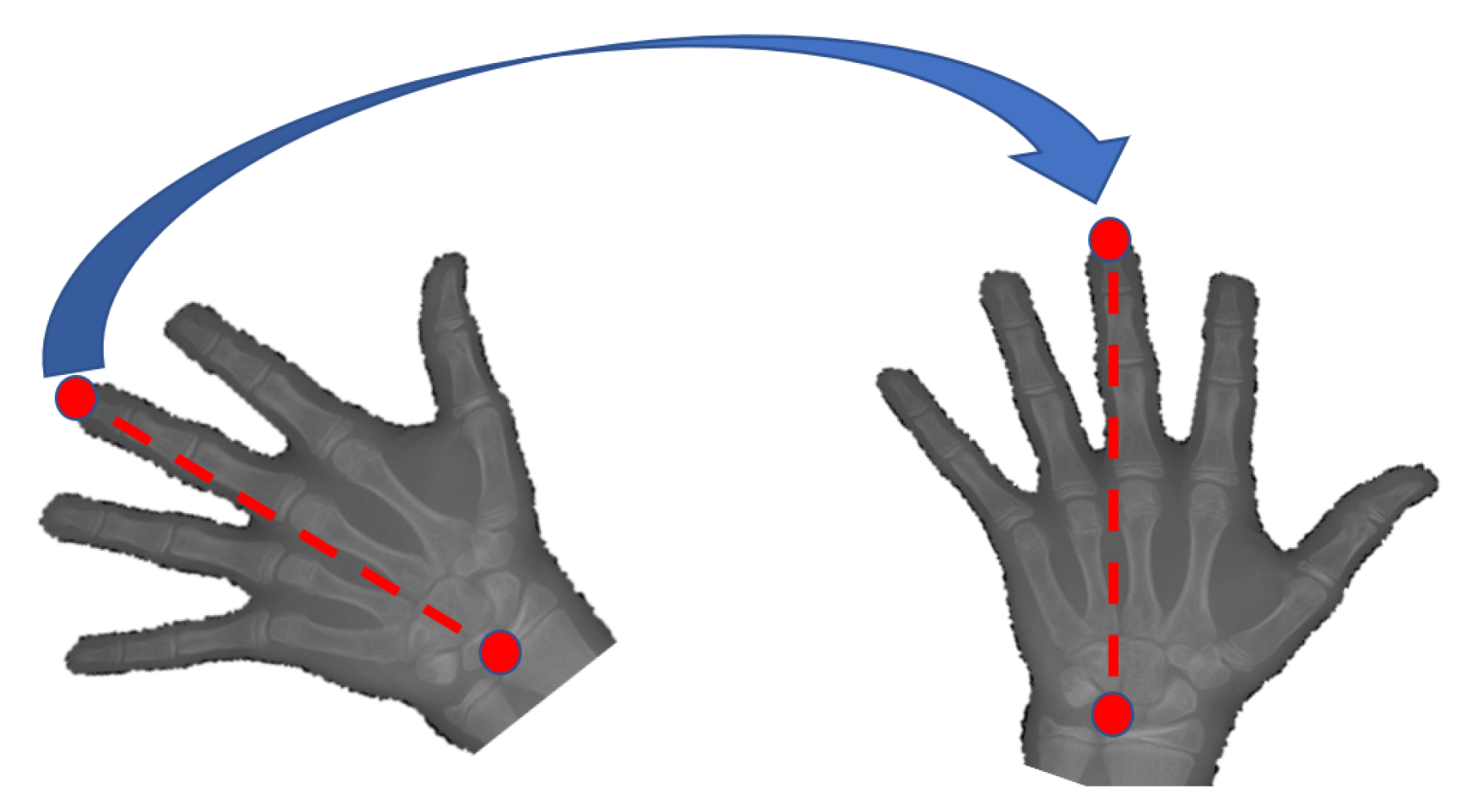
4.1. Data Normalization
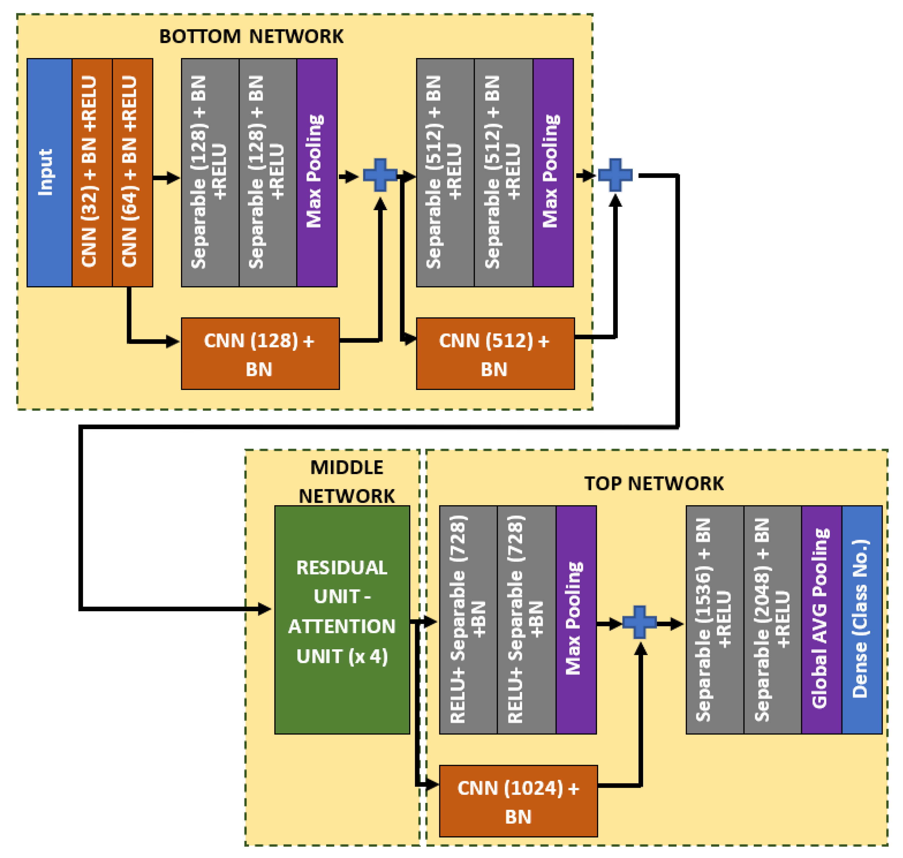
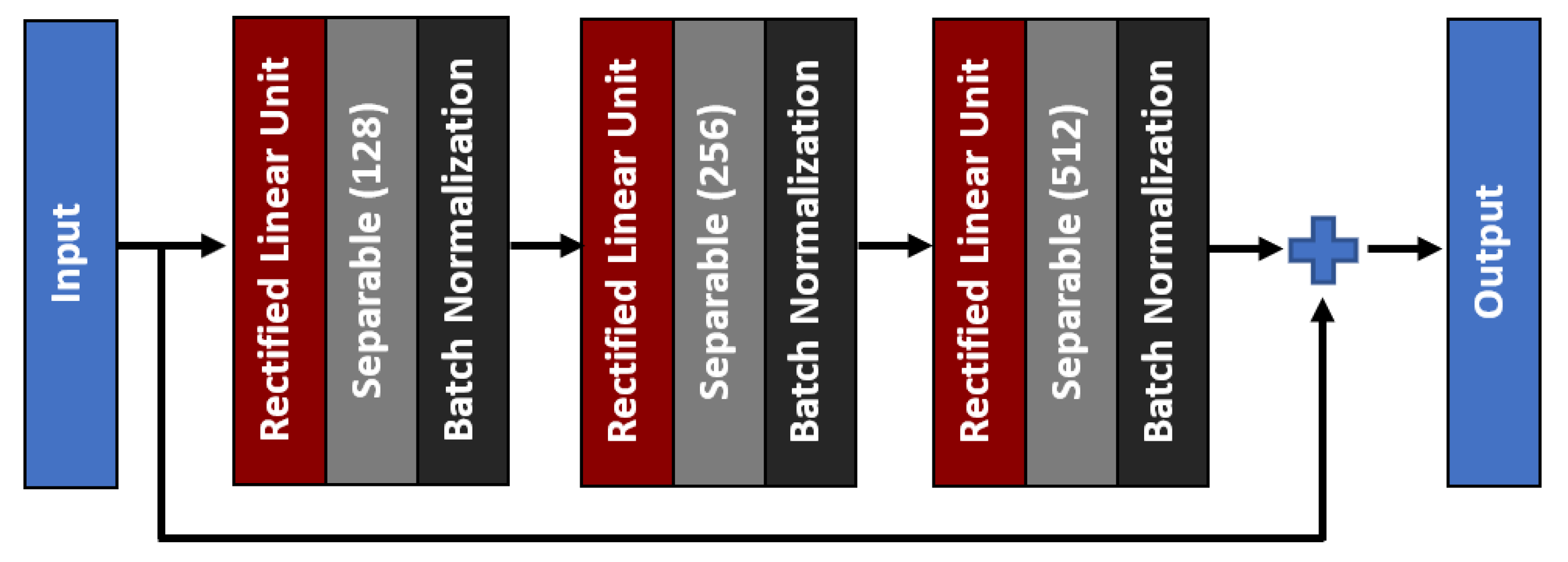
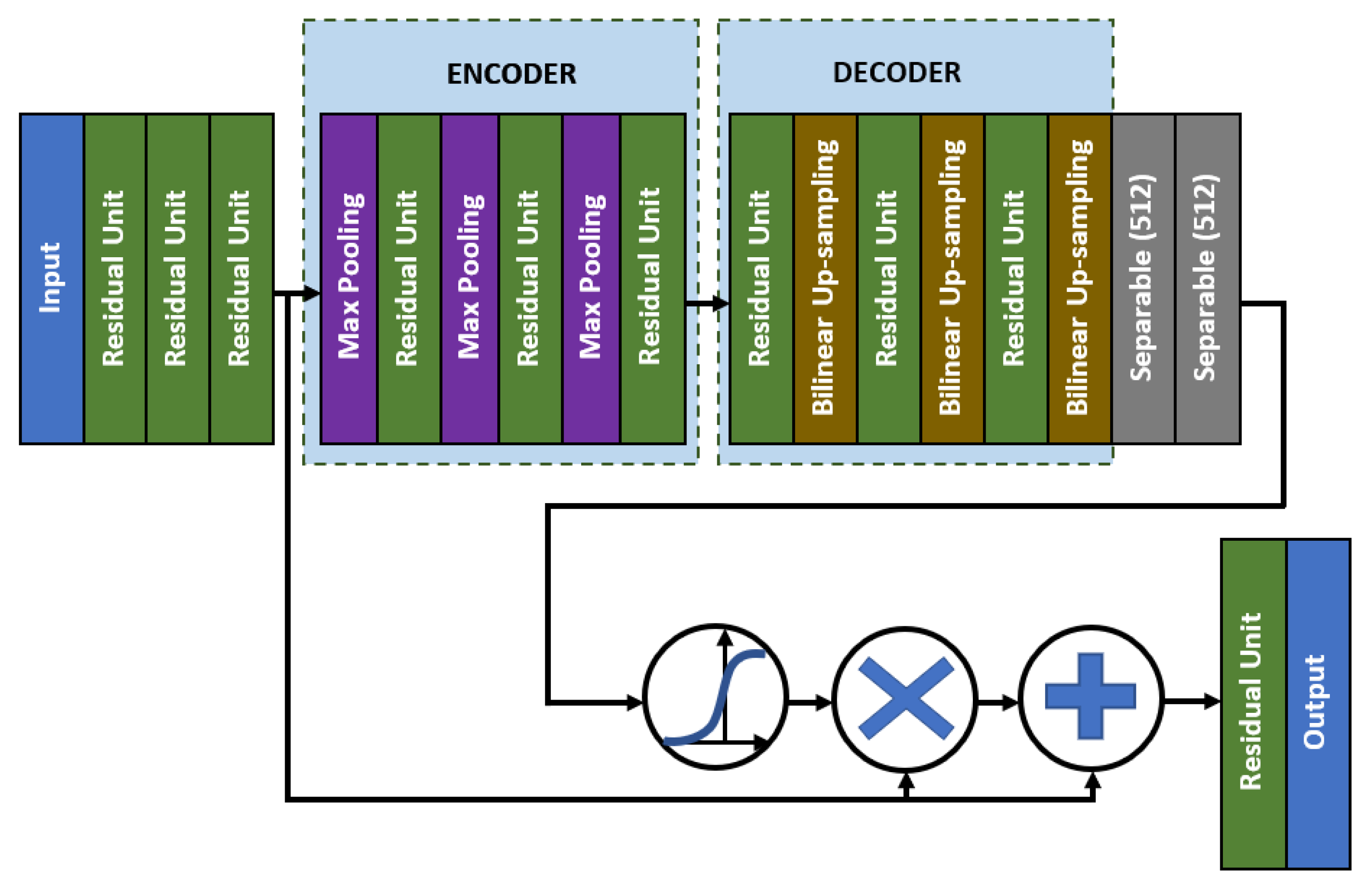
4.2. Bone Age Regression
5. Results and Discussion
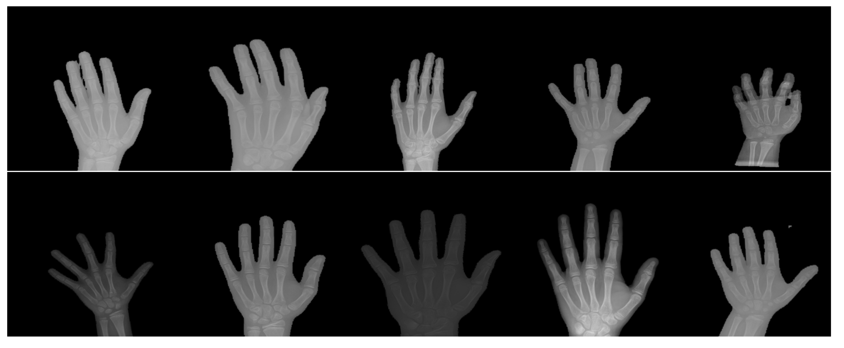
5.1. Dataset
5.2. Training Configurations
5.3. Performance Metrics
5.4. Results and Discussion: Hand Masked Segmentation
5.5. Results and Discussion: Key-Points Detection
5.6. Results and Discussion: Bone Age Assessment
5.7. Results and Discussion: Ablation Study
6. Conclusions
7. Limitation and Future Work
Author Contributions
Funding
Institutional Review Board Statement
Informed Consent Statement
Data Availability Statement
Conflicts of Interest
Abbreviations
| GP | Greulich–Pyle |
| TW | Tanner–Whitehouse |
| AXNet | Attention-Xception Network |
| ROIs | Regions of interest |
| ANN | Artificial Neural Networks |
| CNN | Convolutional Neural Network |
| GPU | Graphics Processing Unit |
References
- Iglovikov, V.I.; Rakhlin, A.; Kalinin, A.A.; Shvets, A.A. Paediatric bone age assessment using deep convolutional neural networks. In Deep Learning in Medical Image Analysis and Multimodal Learning for Clinical Decision Support; Springer: Cham, Switzerland, 2018; pp. 300–308. [Google Scholar]
- Ren, X.; Li, T.; Yang, X.; Wang, S.; Ahmad, S.; Xiang, L.; Stone, S.R.; Li, L.; Zhan, Y.; Shen, D.; et al. Regression convolutional neural network for automated pediatric bone age assessment from hand radiograph. IEEE J. Biomed. Health Inform. 2018, 23, 2030–2038. [Google Scholar] [CrossRef] [PubMed]
- Mutasa, S.; Chang, P.D.; Ruzal-Shapiro, C.; Ayyala, R. MABAL: A novel deep-learning architecture for machine-assisted bone age labeling. J. Digit. Imaging 2018, 31, 513–519. [Google Scholar] [CrossRef] [PubMed]
- Hao, P.; Chen, Y.; Chokuwa, S.; Wu, F.; Bai, C. Skeletal bone age assessment based on deep convolutional neural networks. In Pacific Rim Conference on Multimedia; Springer: Cham, Switherland, 2018; pp. 408–417. [Google Scholar]
- Liu, Y.; Zhang, C.; Cheng, J.; Chen, X.; Wang, Z.J. A multi-scale data fusion framework for bone age assessment with convolutional neural networks. Comput. Biol. Med. 2019, 108, 161–173. [Google Scholar] [CrossRef]
- Guo, J.; Zhu, J.; Du, H.; Qiu, B. A bone age assessment system for real-world X-ray images based on convolutional neural networks. Comput. Electr. Eng. 2020, 81, 106529. [Google Scholar] [CrossRef]
- Abdani, S.R.; Zulkifley, M.A.; Zulkifley, N.H. A Lightweight Deep Learning Model for Covid-19 Detection. In Proceedings of the 2020 IEEE Symposium on Industrial Electronics and Applications (ISIEA), Kristiansand, Norway, 9–13 November 2020; pp. 1–5. [Google Scholar]
- Zulkifley, M.A.; Abdani, S.R.; Zulkifley, N.H. COVID-19 Screening Using a Lightweight Convolutional Neural Network with Generative Adversarial Network Data Augmentation. Symmetry 2020, 12, 1530. [Google Scholar] [CrossRef]
- Asnaoui, K.E.; Chawki, Y.; Idri, A. Automated methods for detection and classification pneumonia based on x-ray images using deep learning. arXiv 2020, arXiv:2003.14363. [Google Scholar]
- Mittal, A.; Kumar, D.; Mittal, M.; Saba, T.; Abunadi, I.; Rehman, A.; Roy, S. Detecting Pneumonia Using Convolutions and Dynamic Capsule Routing for Chest X-ray Images. Sensors 2020, 20, 1068. [Google Scholar] [CrossRef]
- Gornale, S.S.; Patravali, P.U.; Uppin, A.M.; Hiremath, P.S. Study of Segmentation Techniques for Assessment of Osteoarthritis in Knee X-ray Images. Int. J. Image Graph. Signal Process. (IJIGSP) 2019, 11, 48–57. [Google Scholar] [CrossRef]
- Brahim, A.; Jennane, R.; Riad, R.; Janvier, T.; Khedher, L.; Toumi, H.; Lespessailles, E. A decision support tool for early detection of knee OsteoArthritis using X-ray imaging and machine learning: Data from the OsteoArthritis Initiative. Comput. Med Imaging Graph. 2019, 73, 11–18. [Google Scholar] [CrossRef]
- Bouchahma, M.; Hammouda, S.B.; Kouki, S.; Alshemaili, M.; Samara, K. An Automatic Dental Decay Treatment Prediction using a Deep Convolutional Neural Network on X-Ray Images. In Proceedings of the 16th International Conference on Computer Systems and Applications (AICCSA), Abu Dhabi, United Arab Emirates, 3–7 November 2019; pp. 1–4. [Google Scholar]
- Tuan, T.M.; Fujita, H.; Dey, N.; Ashour, A.S.; Ngoc, V.T.N.; Chu, D.T. Dental diagnosis from X-ray images: An expert system based on fuzzy computing. Biomed. Signal Process. Control. 2018, 39, 64–73. [Google Scholar]
- Takahashi, T.; Kokubun, M.; Mitsuda, K.; Kelley, R.; Ohashi, T.; Aharonian, F.; Akamatsu, H.; Akimoto, F.; Allen, S.; Anabuki, N.; et al. The ASTRO-H (Hitomi) X-ray Astronomy Satellite. In Proceedings of the Space Telescopes and Instrumentation 2016: Ultraviolet to Gamma Ray, Edinburgh, UK, 26 June–1 July 2016; Volume 9905, p. 99050U. [Google Scholar]
- Nazri, N.; Annuar, A. X-ray Sources Population in NGC 1559. J. Kejuruter. 2020, 3, 7–14. [Google Scholar]
- Sazhin, M.V.; Zharov, V.E.; Milyukov, V.K.; Pshirkov, M.S.; Sementsov, V.N.; Sazhina, O.S. Space Navigation by X-ray Pulsars. Mosc. Univ. Phys. Bull. 2018, 73, 141–153. [Google Scholar] [CrossRef]
- Greulich, W.W.; Pyle, S.I. Radiographic Atlas of Skeletal Development of the Hand and Wrist; Stanford University Press: Palo Alto, CA, USA, 1959. [Google Scholar]
- Breen, M.A.; Tsai, A.; Stamm, A.; Kleinman, P.K. Bone age assessment practices in infants and older children among Society for Pediatric Radiology members. Pediatr. Radiol. 2016, 46, 1269–1274. [Google Scholar] [CrossRef]
- Tanner, J.M.; Whitehouse, R.H.; Cameron, N.; Marshall, W.A.; Healy, M.J.R.; Goldstein, H. Assessment of skeletal maturity and prediction of adult height (TW2 method); Saunders: London, UK, 2001; pp. 1–110. [Google Scholar]
- Nadeem, M.W.; Goh, H.G.; Ali, A.; Hussain, M.; Khan, M.A. Bone Age Assessment Empowered with Deep Learning: A Survey, Open Research Challenges and Future Directions. Diagnostics 2020, 10, 781. [Google Scholar] [CrossRef] [PubMed]
- Mohamed, N.A.; Zulkifley, M.A.; Kamari, N.A.M. Convolutional Neural Networks Tracker with Deterministic Sampling for Sudden Fall Detection. In Proceedings of the 2019 IEEE 9th International Conference on System Engineering and Technology (ICSET), Shah Alam, Malaysia, 7 October 2019; pp. 1–5. [Google Scholar]
- Nevavuori, P.; Narra, N.; Lipping, T. Crop yield prediction with deep convolutional neural networks. Comput. Electron. Agric. 2019, 163, 104859. [Google Scholar] [CrossRef]
- Guo, J.; He, H.; He, T.; Lausen, L.; Li, M.; Lin, H.; Shi, X.; Wang, C.; Xie, J.; Zha, S.; et al. GluonCV and GluonNLP: Deep Learning in Computer Vision and Natural Language Processing. J. Mach. Learn. Res. 2020, 21, 1–7. [Google Scholar]
- Zulkifley, M.A.; Mohamed, N.A.; Zulkifley, N.H. Squat angle assessment through tracking body movements. IEEE Access 2019, 7, 48635–48644. [Google Scholar] [CrossRef]
- Mohamed, N.A.; Zulkifley, M.A.; Abdani, S.R. Spatial Pyramid Pooling with Atrous Convolutional for MobileNet. In Proceedings of the IEEE Student Conference on Research and Development (SCOReD), Johor, Malaysia, 27–29 September 2020; pp. 333–336. [Google Scholar]
- Nazi, Z.A.; Abir, T.A. Automatic Skin Lesion Segmentation and Melanoma Detection: Transfer Learning Approach with U-NET and DCNN-SVM. In Proceedings of the International Joint Conference on Computational Intelligence, Budapest, Hungary, 2–4 November 2020; Springer: Singapore; pp. 371–381. [Google Scholar]
- Spampinato, C.; Palazzo, S.; Giordano, D.; Aldinucci, M.; Leonardi, R. Deep learning for automated skeletal bone age assessment in X-ray images. Med Image Anal. 2017, 36, 41–51. [Google Scholar] [CrossRef] [PubMed]
- Lee, H.; Tajmir, S.; Lee, J.; Zissen, M.; Yeshiwas, B.A.; Alkasab, T.K.; Choy, G.; Do, S. Fully automated deep learning system for bone age assessment. J. Digit. Imaging 2017, 30, 427–441. [Google Scholar] [CrossRef] [PubMed]
- Zulkifley, M.A.; Abdani, S.R.; Zulkifley, N.H. Automated Bone Age Assessment with Image Registration Using Hand X-ray Images. Appl. Sci. 2020, 10, 7233. [Google Scholar] [CrossRef]
- Dallora, A.L.; Anderberg, P.; Kvist, O.; Mendes, E.; Ruiz, S.D.; Berglund, J.S. Bone age assessment with various machine learning techniques: A systematic literature review and meta-analysis. PLoS ONE 2019, 14, e0220242. [Google Scholar] [CrossRef]
- Cunha, P.; Moura, D.C.; López, M.A.G.; Guerra, C.; Pinto, D.; Ramos, I. Impact of ensemble learning in the assessment of skeletal maturity. J. Med Syst. 2014, 38, 1–10. [Google Scholar] [CrossRef] [PubMed]
- Luca, S.D.; Mangiulli, T.; Merelli, V.; Conforti, F.; Palacio, L.A.V.; Agostini, S.; Spinas, E.; Cameriere, R. A new formula for assessing skeletal age in growing infants and children by measuring carpals and epiphyses of radio and ulna. J. Forensic Leg. Med. 2016, 39, 109–116. [Google Scholar] [CrossRef]
- Tang, F.H.; Chan, J.L.; Chan, B.K. Accurate age determination for adolescents using magnetic resonance imaging of the hand and wrist with an artificial neural network-based approach. J. Digit. Imaging 2019, 32, 283–289. [Google Scholar] [CrossRef]
- Pahuja, M.; Garg, N.K. Skeleton Bone Age Assessment using Optimized Artificial Neural Network. In Proceedings of the 3rd IEEE International Conference on Recent Trends in Electronics, Information and Communication Technology (RTEICT), Bengaluru, India, 18–19 May 2018; pp. 623–629. [Google Scholar]
- Kashif, M.; Deserno, T.M.; Haak, D.; Jonas, S. Feature description with SIFT, SURF, BRIEF, BRISK, or FREAK? A general question answered for bone age assessment. Comput. Biol. Med. 2016, 68, 67–75. [Google Scholar] [CrossRef] [PubMed]
- Sheshasaayee, A.; Jasmine, C. A Novel Pre-processing and Kernel Based Support Vector Machine Classifier with Discriminative Dictionary Learning for Bone Age Assessment. Res. J. Appl. Sci. Eng. Technol. 2016, 12, 933–946. [Google Scholar] [CrossRef]
- Simu, S.; Lal, S. Automated Bone Age Assessment using Bag of Features and Random Forests. In Proceedings of the 2017 International Conference on Intelligent Sustainable Systems (ICISS), Palladam, India, 7–8 December 2017; pp. 911–915. [Google Scholar]
- Zhou, J.; Li, Z.; Zhi, W.; Liang, B.; Moses, D.; Dawes, L. Using Convolutional Neural Networks and Transfer Learning for Bone Age Classification. In Proceedings of the 2017 International Conference on Digital Image Computing: Techniques and Applications (DICTA), Sydney, Australia, 29 November–1 December 2017; pp. 1–6. [Google Scholar]
- Wibisono, A.; Mursanto, P. Multi Region-Based Feature Connected Layer (RB-FCL) of deep learning models for bone age assessment. J. Big Data 2020, 7, 1–17. [Google Scholar] [CrossRef]
- Tang, W.; Wu, G.; Shen, G. Improved Automatic Radiographic Bone Age Prediction with Deep Transfer Learning. In Proceedings of the 12th International Congress on Image and Signal Processing, BioMedical Engineering and Informatics (CISP-BMEI), Suzhou, China, 19–21 October 2019; pp. 1–6. [Google Scholar]
- Chen, C.; Chen, Z.; Jin, X.; Li, L.; Speier, W.; Arnold, C.W. Attention-Guided Discriminative Region Localization for Bone Age Assessment. arXiv 2020, arXiv:2006.00202, 1–9. [Google Scholar]
- Wu, E.; Kong, B.; Wang, X.; Bai, J.; Lu, Y.; Gao, F.; Zhang, S.; Cao, K.; Song, Q.; Lyu, S.; et al. Residual Attention Based Network for Hand Bone Age Assessment. In Proceedings of the 2019 IEEE 16th International Symposium on Biomedical Imaging (ISBI), Venice, Italy, 8–11 April 2019; pp. 1158–1161. [Google Scholar]
- Reddy, N.E.; Rayan, J.C.; Annapragada, A.V.; Mahmood, N.F.; Scheslinger, A.E.; Zhang, W.; Kan, J.H. Bone age determination using only the index finger: A novel approach using a convolutional neural network compared with human radiologists. Pediatr. Radiol. 2020, 50, 516–523. [Google Scholar] [CrossRef]
- Marouf, M.; Siddiqi, R.; Bashir, F.; Vohra, B. Automated Hand X-Ray Based Gender Classification and Bone Age Assessment Using Convolutional Neural Network. In Proceedings of the 3rd International Conference on Computing, Mathematics and Engineering Technologies (iCoMET), Sukkur, Pakistan, 29–30 January 2020; pp. 1–5. [Google Scholar]
- Pan, X.; Zhao, Y.; Chen, H.; Wei, D.; Zhao, C.; Wei, Z. Fully automated bone age assessment on large-scale hand X-ray dataset. Int. J. Biomed. Imaging 2020, 1–12. [Google Scholar] [CrossRef]
- Hao, G.; Li, Y. Bone Age Estimation with X-ray Images Based on EfficientNet Pre-training Model. J. Physics Conf. Ser. 2021, 1827, 1–8. [Google Scholar] [CrossRef]
- Shah, S.; Ghosh, P.; Davis, L.S.; Goldstein, T. Stacked U-Nets: A no-frills approach to natural image segmentation. arXiv 2018, arXiv:1804.10343. [Google Scholar]
- Zhao, H.; Shi, J.; Qi, X.; Wang, X.; Jia, J. Pyramid Scene Parsing Network. In Proceedings of the IEEE Conference on Computer Vision and Pattern Recognition, Honolulu, HI, USA, 21–26 July 2017; pp. 2881–2890. [Google Scholar]
- Abdani, S.R.; Zulkifley, M.A.; Moubark, A.M. Pterygium Tissues Segmentation using Densely Connected Deeplab. In Proceedings of the 2020 IEEE 10th Symposium on Computer Applications and Industrial Electronics (ISCAIE), Penang, Malaysia, 18–19 April 2020; pp. 229–232. [Google Scholar]
- Long, J.; Shelhamer, E.; Darrell, T. Fully Convolutional Networks for Semantic Segmentation. In Proceedings of the IEEE conference on computer vision and pattern recognition, Boston, MA, USA, 7–12 June 2015; pp. 3431–3440. [Google Scholar]
- Chen, L.C.; Papandreou, G.; Kokkinos, I.; Murphy, K.; Yuille, A.L. Semantic image segmentation with deep convolutional nets and fully connected crfs. arXiv 2014, arXiv:1412.7062. [Google Scholar]
- Chen, L.C.; Papandreou, G.; Kokkinos, I.; Murphy, K.; Yuille, A.L. Deeplab: Semantic image segmentation with deep convolutional nets, atrous convolution, and fully connected crfs. IEEE Trans. Pattern Anal. Mach. Intell. 2017, 40, 834–848. [Google Scholar] [CrossRef] [PubMed]
- Badrinarayanan, V.; Handa, A.; Cipolla, R. Segnet: A deep convolutional encoder-decoder architecture for robust semantic pixel-wise labelling. arXiv 2015, arXiv:1505.07293. [Google Scholar]
- Jégou, S.; Drozdzal, M.; Vazquez, D.; Romero, A.; Bengio, Y. The One Hundred Layers Tiramisu: Fully Convolutional Densenets for Semantic Segmentation. In Proceedings of the IEEE conference on computer vision and pattern recognition workshops, Honolulu, HI, USA, 21–26 July 2017; pp. 11–19. [Google Scholar]
- Ronneberger, O.; Fischer, P.; Brox, T. U-net: Convolutional Networks for Biomedical Image Segmentation. In Proceedings of the International Conference on Medical image computing and computer-assisted intervention, Munich, Germany, 5–9 October 2015; pp. 234–241. [Google Scholar]
- Chen, L.C.; Zhu, Y.; Papandreou, G.; Schroff, F.; Adam, H. Encoder-Decoder with Atrous Separable Convolution for Semantic Image Segmentation. In Proceedings of the European Conference on Computer Vision (ECCV), Munich, Germany, 8–14 September 2018; pp. 801–818. [Google Scholar]
- He, K.; Zhang, X.; Ren, S.; Sun, J. Deep Residual Learning for Image Recognition. In Proceedings of the IEEE Conference on Computer Vision and Pattern Recognition, Las Vegas, NV, USA, 27–30 June 2016; pp. 770–778. [Google Scholar]
- Szegedy, C.; Liu, W.; Jia, Y.; Sermanet, P.; Reed, S.; Anguelov, D.; Erhan, D.; Vanhoucke, V.; Rabinovich, A. Going Deeper with Convolutions. In Proceedings of the IEEE Conference on Computer Vision and Pattern Recognition, Boston, MA, USA, 7–12 June 12 2015; pp. 1–9. [Google Scholar]
- Zhang, X.; Zhou, X.; Lin, M.; Sun, J. Shufflenet: An Extremely Efficient Convolutional Neural Network for Mobile Devices. In Proceedings of the IEEE Conference on Computer Vision and Pattern Recognition, Salt Lake City, UT, USA, 18–23 June 2018; pp. 6848–6856. [Google Scholar]
- Ma, N.; Zhang, X.; Zheng, H.T.; Sun, J. Shufflenet v2: Practical Guidelines for Efficient CNN Architecture Design. In Proceedings of the European conference on computer vision (ECCV), Munich, Germany, 8–14 September 2018; pp. 116–131. [Google Scholar]
- Howard, A.G.; Zhu, M.; Chen, B.; Kalenichenko, D.; Wang, W.; Weyand, T.; Andreetto, M.; Adam, H. Mobilenets: Efficient convolutional neural networks for mobile vision applications. arXiv 2017, arXiv:1704.04861. [Google Scholar]
- Sandler, M.; Howard, A.; Zhu, M.; Zhmoginov, A.; Chen, L.C. Mobilenetv2: Inverted Residuals and Linear Bottlenecks. In Proceedings of the IEEE Conference on Computer Vision and Pattern Recognition, Salt Lake City, UT, USA, 18–23 June 2018; pp. 4510–4520. [Google Scholar]
- Howard, A.; Sandler, M.; Chu, G.; Chen, L.C.; Chen, B.; Tan, M.; Wang, W.; Zhu, Y.; Pang, R.; Vasudevan, V.; et al. Searching for Mobilenetv3. In Proceedings of the IEEE/CVF International Conference on Computer Vision, Seoul, Korea, 27 October–2 November 2019; pp. 1314–1324. [Google Scholar]
- Iandola, F.N.; Han, S.; Moskewicz, M.W.; Ashraf, K.; Dally, W.J.; Keutzer, K. SqueezeNet: AlexNet-level accuracy with 50× fewer parameters and< 0.5 MB model size. arXiv 2016, arXiv:1602.07360. [Google Scholar]
- Chollet, F. Xception: Deep Learning with Depthwise Separable Convolutions. In Proceedings of the IEEE Conference on Computer Vision and Pattern Recognition, Honolulu, HI, USA, 21–26 July 2017; pp. 1251–1258. [Google Scholar]
- Huang, G.; Liu, Z.; Maaten, L.V.D.; Weinberger, K.Q. Densely Connected Convolutional Networks. In Proceedings of the IEEE Conference on Computer Vision and Pattern Recognition, Honolulu, HI, USA, 21–26 July 2017; pp. 4700–4708. [Google Scholar]
- Halabi, S.S.; Prevedello, L.M.; Kalpathy-Cramer, J.; Mamonov, A.B.; Bilbily, A.; Cicero, M.; Pan, I.; Pereira, L.A.; Sousa, R.T.; Abdala, N.; et al. The RSNA pediatric bone age machine learning challenge. Radiology 2019, 290, 498–503. [Google Scholar] [CrossRef] [PubMed]
- Wu, Y.; He, K. Group Normalization. In Proceedings of the European Conference on Computer Vision (ECCV), Munich, Germany, 8–14 September 2018; pp. 3–19. [Google Scholar]
- Simonyan, K.; Zisserman, A. Very deep convolutional networks for large-scale image recognition. arXiv 2014, arXiv:1409.1556. [Google Scholar]
- Szegedy, C.; Vanhoucke, V.; Ioffe, S.; Shlens, J.; Wojna, Z. Rethinking the Inception Architecture for Computer Vision. In Proceedings of the IEEE Conference on Computer Vision and Pattern Recognition, Las Vegas, NV, USA, 27–30 June 2016; pp. 2818–2826. [Google Scholar]


| Method | Model | Strength | Weakness |
|---|---|---|---|
| Spampinato et al. [28] | BoNet | -Uses a simple CNN architecture with only five convolutional layers. | -Does not employ any pre-processing pipeline. -Does not embed residual or feed-forward connections. |
| Lee et al. [29] | GoogLeNet | -Applies pre-processing pipeline to produce standardized images. | -The experiment has included radiologists report for training process, which will give advantage for bone age prediction performance. |
| Zhou et al. [39] | CNNs | -Uses various ROIs based on domain knowledge to increase model accuracy. | -The model is not trained until convergence because the model accuracy is still increasing before the training has been ended. |
| Wibisono and Mursanto [40] | DenseNet and InceptionResNet V2 | -The hand X-ray images are divided into five different deep learning models are used to produce the feature maps. | -Not an end-to-end model since the bone age prediction is performed using Random Forest regressor technique. |
| Tang et al. [41] | CNNs | -Applies transfer learning to mitigate small training data. | -Does not perform any hyperparameter tuning. |
| Iglovikov et al. [1] | VGGNet | -Introduces image registration pipeline which includes hand segmentation, normalizing contrast, and key points detection. | -The model does not apply residual or feed-forward connections. |
| Chen et al. [42] | Inception-V3 | -Applies attention guided method to localize three different regions using image-level labels. | -The system has applied gender information, which will give advantage for bone age prediction performance. |
| Reddy et al. [44] | CNNs | -Uses information of index finger only to train the CNNs architecture. | -Does not employ any pre-processing pipeline. |
| Marouf et al. [45] | CNNs | -Applies gender information in the model training process. | -Training accuracy and loss still fluctuate a lot for before the training has been ended. |
| Pan et al. [46] | InceptionResnet-V2 | -Uses active learning to alleviate the annotation burden. -Applies transfer learning technique. | -The computational complexity is large due to ensembling process of hand masked segmentation and prediction module. |
| Hao and Li [47] | EfficientNet | -Applies pre-processing pipeline that include resizing, normalization, and data enhancement to remove bias and increase the number of training data. | -The experiment has included gender information which will give advantage for bone age prediction. |
| Layer | Operator | Resolution | Channel | Kernel | Pool | Skip Connection |
|---|---|---|---|---|---|---|
| 1 | Convolution | 288 × 288 | 32 | 3 × 3 | No | No |
| 2 | Convolution | 144 × 144 | 64 | 3 × 3 | No | No |
| 3 | Separable convolution | 144 × 144 | 128 | 3 × 3 | No | No |
| 4 | Separable convolution | 144 × 144 | 128 | 3 × 3 | Yes | Yes |
| 5 | Separable convolution | 72 × 72 | 256 | 3 × 3 | No | No |
| 6 | Separable convolution | 72 × 72 | 256 | 3 × 3 | Yes | Yes |
| 7 | Residual | 24 × 24 | 128 | 1 × 1 | No | Yes |
| Unit | 256 | 3 × 3 | ||||
| 512 | 1 × 1 | |||||
| 8 | Attention | 24 × 24 | All | 3 × 3 | 3 Downpool | Yes |
| Unit | 512 | + | ||||
| 3 Upsample | ||||||
| 9 | Residual | 24 × 24 | 128 | 1 × 1 | No | Yes |
| Unit | 256 | 3 × 3 | ||||
| 512 | 1 × 1 | |||||
| 10 | Attention | 24 × 24 | All | 3 × 3 | 3 Downpool | Yes |
| Unit | 512 | + | ||||
| 3 Upsample | ||||||
| 11 | Residual | 24 × 24 | 128 | 1 × 1 | No | Yes |
| Unit | 256 | 3 × 3 | ||||
| 512 | 1 × 1 | |||||
| 12 | Attention | 24 × 24 | All | 3 × 3 | 3 Downpool | Yes |
| Unit | 512 | + | ||||
| 3 Upsample | ||||||
| 13 | Residual | 24 × 24 | 128 | 1 × 1 | No | Yes |
| Unit | 256 | 3 × 3 | ||||
| 512 | 1 × 1 | |||||
| 14 | Attention | 24 × 24 | All | 3 × 3 | 3 Downpool | Yes |
| Unit | 512 | + | ||||
| 3 Upsample | ||||||
| 15 | Separable convolution | 24 × 24 | 728 | 3 × 3 | No | No |
| 16 | Separable convolution | 24 × 24 | 1024 | 3 × 3 | Yes | Yes |
| 17 | Separable convolution | 12 × 12 | 1536 | 3 × 3 | No | No |
| 18 | Global pPool + Dense | 1 × 1 | 2048 | 1 × 1 | Yes | No |
| Method | (%) | IoU | Total No. of Parameters (Unit Register) | (Pixels) |
|---|---|---|---|---|
| Stacked U-Net [48] | 95.330 | 0.88967 | 3,036,802 | 40.848 |
| PSPNet [49] | 97.084 | 0.93094 | 27,896,000 | 7.625 |
| DenseDeepLab V2 [50] | 97.153 | 0.93234 | 110,054,344 | 3.558 |
| FCN [51] | 97.156 | 0.93253 | 134,393,428 | 2.747 |
| DeepLab V1 [52] | 97.198 | 0.93339 | 28,890,946 | 3.358 |
| DeepLab V2 [53] | 97.226 | 0.93405 | 71,419,720 | 3.606 |
| DenseDeepLab V1 [50] | 97.297 | 0.93565 | 40,900,546 | 3.368 |
| SegNet [54] | 97.709 | 0.94507 | 29,460,042 | 3.408 |
| FC DenseNet [55] | 97.741 | 0.94568 | 14,729,860 | 3.450 |
| U-Net [56] | 97.809 | 0.94739 | 31,032,834 | 2.897 |
| DeepLab V3+ [57] | 97.826 | 0.94778 | 41,253,888 | 3.791 |
| Method | MAE (Pixels) | MSE (Pixels) | Total No. of. Parameters (Unit Register) |
|---|---|---|---|
| ResNet-50 [58] | 0.12444 | 0.04091 | 23,577544 |
| GoogleNet [59] | 0.12410 | 0.13668 | 10,326,527 |
| ShuffleNet V1 [60] | 0.08183 | 0.02219 | 947,216 |
| MobileNet V2 [63] | 0.07564 | 0.02466 | 2,269,384 |
| SqueezeNet [65] | 0.06448 | 0.02091 | 739,600 |
| MobileNet V3 [64] | 0.05699 | 0.02098 | 3,795,832 |
| ShuffleNet V2 [61] | 0.05473 | 0.01999 | 5,395,104 |
| LightCovidNet [8] | 0.05028 | 0.01789 | 890,416 |
| Xception-41 [66] | 0.04913 | 0.01571 | 20,877,872 |
| Xception-71 [66] | 0.04776 | 0.01572 | 35,640,704 |
| SPPCovidNet [7] | 0.04389 | 0.01452 | 910,976 |
| DenseNet-264 [67] | 0.04138 | 0.01577 | 31,068,744 |
| MobileNet V1 [62] | 0.03563 | 0.01409 | 3,237,064 |
| Method | MAE (Months) | MSE (Months) | Total No. of Parameters (Unit Register) |
|---|---|---|---|
| ShuffleNet V1 [60] | 15.728 | 372.575 | 936,457 |
| Iglovikov et al. [1] | 14.804 | 349.254 | 33,601,345 |
| SqueezeNet [65] | 14.164 | 311.783 | 735,939 |
| VGG-19 [70] | 14.028 | 307.416 | 38,911,041 |
| MobileNet V3 small [64] | 13.541 | 282.157 | 1,662,939 |
| Hao and Li [47] | 12.331 | 250.321 | 12,757,296 |
| MobileNet V2 large [64] | 12.307 | 242.316 | 3,786,865 |
| ShuffleNet V2 [61] | 12.010 | 226.951 | 5,380,761 |
| MobileNet V2 [63] | 11.394 | 213.454 | 2,260,417 |
| Spampinato et al. [28] | 11.173 | 205.067 | 95,116,161 |
| Lee et al. [29] | 10.972 | 220.759 | 5,973,224 |
| MobileNet V1 [62] | 10.886 | 190.349 | 3,229,889 |
| DenseNet [67] | 10.557 | 190.105 | 31,049,529 |
| ResNet [58] | 10.283 | 264.660 | 23,563,201 |
| Inception V3 [71] | 9.774 | 191.696 | 18,783,649 |
| Pan et al. [46] | 9.587 | 152.328 | 54,336,736 |
| Xception-41 [66] | 8.357 | 121.155 | 20,863,529 |
| Zulkifley et al. [30] | 8.200 | 121.902 | 20,863,529 |
| AXNet | 7.699 | 108.869 | 21,035,545 |
| Method | MAE (Months) | MSE (Months) |
|---|---|---|
| AXNet without attention unit | 8.357 | 121.155 |
| AXNet without data normalization | 8.219 | 119.240 |
| AXNet | 7.699 | 108.869 |
Publisher’s Note: MDPI stays neutral with regard to jurisdictional claims in published maps and institutional affiliations. |
© 2021 by the authors. Licensee MDPI, Basel, Switzerland. This article is an open access article distributed under the terms and conditions of the Creative Commons Attribution (CC BY) license (https://creativecommons.org/licenses/by/4.0/).
Share and Cite
Zulkifley, M.A.; Mohamed, N.A.; Abdani, S.R.; Kamari, N.A.M.; Moubark, A.M.; Ibrahim, A.A. Intelligent Bone Age Assessment: An Automated System to Detect a Bone Growth Problem Using Convolutional Neural Networks with Attention Mechanism. Diagnostics 2021, 11, 765. https://doi.org/10.3390/diagnostics11050765
Zulkifley MA, Mohamed NA, Abdani SR, Kamari NAM, Moubark AM, Ibrahim AA. Intelligent Bone Age Assessment: An Automated System to Detect a Bone Growth Problem Using Convolutional Neural Networks with Attention Mechanism. Diagnostics. 2021; 11(5):765. https://doi.org/10.3390/diagnostics11050765
Chicago/Turabian StyleZulkifley, Mohd Asyraf, Nur Ayuni Mohamed, Siti Raihanah Abdani, Nor Azwan Mohamed Kamari, Asraf Mohamed Moubark, and Ahmad Asrul Ibrahim. 2021. "Intelligent Bone Age Assessment: An Automated System to Detect a Bone Growth Problem Using Convolutional Neural Networks with Attention Mechanism" Diagnostics 11, no. 5: 765. https://doi.org/10.3390/diagnostics11050765
APA StyleZulkifley, M. A., Mohamed, N. A., Abdani, S. R., Kamari, N. A. M., Moubark, A. M., & Ibrahim, A. A. (2021). Intelligent Bone Age Assessment: An Automated System to Detect a Bone Growth Problem Using Convolutional Neural Networks with Attention Mechanism. Diagnostics, 11(5), 765. https://doi.org/10.3390/diagnostics11050765