
Forecasting the Walking Assistance Rehabilitation Level of Stroke Patients Using Artificial Intelligence

 ,
,  ,
,
Abstract
1. Introduction
2. Dataset and Experimental Settings
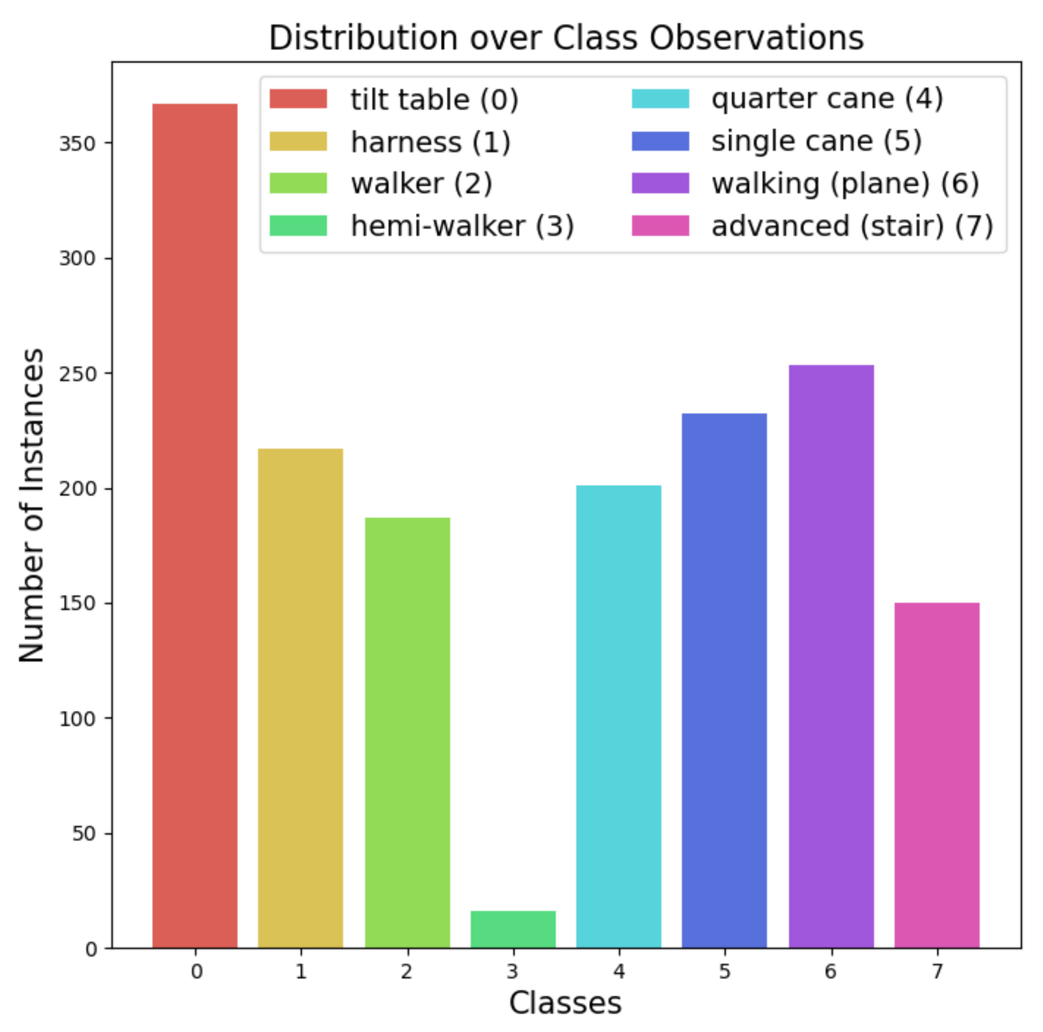
2.1. Data Description
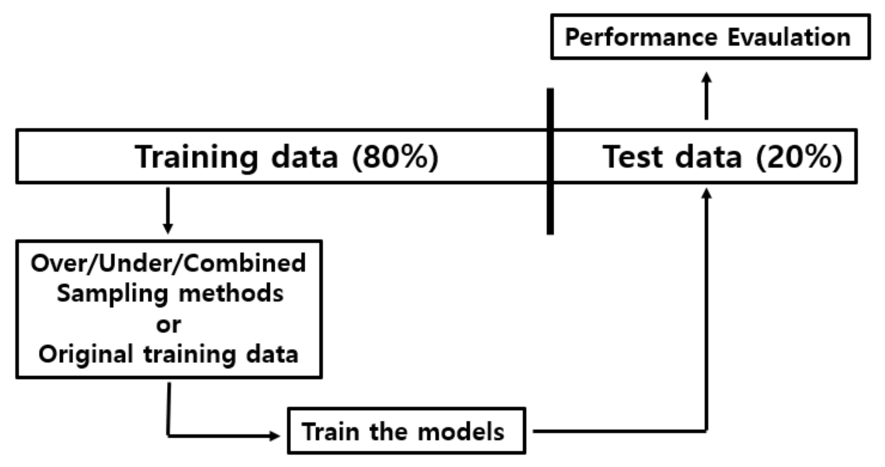
2.2. Data Preprocessing: Undersampling, Oversampling, and Combined Sampling Methods
2.3. ML and DL Algorithm Settings
- LightGBM settings: in the LightGBM package (Ver. 2.3.1) provided as Python API via scikit-learn [23,24], we empirically decided to use a traditional gradient boosting decision tree as a boosting type without limitations for the number of leaf nodes and depth. We also found that the best performing learning rate was 0.1.
- AutoGluon settings: among the various AutoML Python library packages, we employed the latest and best performing one: AutoGluon (Ver. 0.0.15) [29]. We empirically adjusted the “time_limit” parameter for the whole model from 60 to 120 s and found that the performance did not improve over 120 s. The evaluation metric for each model in the ensemble was set to “accuracy”. We also set the “presets” parameter to be “best_quality” to improve the ensemble models’ predictive performance based on stacking and bagging in the granted training time.
- SuperTML settings: as this model transforms tabular data into images, its performance depends on convolutional structures. Therefore, we experimentally found that ResNet [2] with 152 convolutional layers performed the best.
- TabNet settings: although TabNet [31] is composed of an encoder and a decoder for self-supervised learning [33], we employed only its encoder network for supervised learning. To improve its predictive performance, we modified it into a six-step operation, where we omitted “shared across decision steps” at steps 1–3 under the feature transformer process. We also changed the shared across decision steps to unshared across decision steps in steps 4–6.
2.4. Performance Measurement Settings
3. Results and Discussion
3.1. Classification Results of ML and DL Models
3.2. Which Model Performed Best?
4. Conclusions
Author Contributions
Funding
Institutional Review Board Statement
Informed Consent Statement
Data Availability Statement
Conflicts of Interest
Appendix A. Background of the Sampling Methods and Classification Models
Appendix A.1. Background of the Sampling Methods
- Oversampling (SMOTE): proposed by Chawla et al. [19], the synthetic minority oversampling technique (SMOTE) first chooses a single instance a from a minor class at random and arbitrarily selects a single instance b that is k-nearest to a. Then, it draws lines between them, on which a new synthetic instance is generated iteratively via a convex combination of a and b.
- Undersampling (TomekLinks): the concept of “TomekLinks” is defined via satisfaction of the following conditions, for instance, for a and b [20]: (1) The two observations are the closest neighbors to each other measured by Euclidean distance. (2) They belong to different class labels (e.g., a is in the minor class while b is in the major class, and vice versa). Then, the observations in the major class, considered as ambiguous examples, are removed to balance the class distribution.
Appendix A.2. Background of the Classification Methods
- Support vector machines (SVM): SVM for classification [42] aims to find a proper hyperplane that best separates the instances into different classes. In other words, it tries to find a support vector that is orthogonal and maximizes the margin to the hyperplane. SVM uses some kernel tricks to replace the dot product of two vectors with the kernel function.
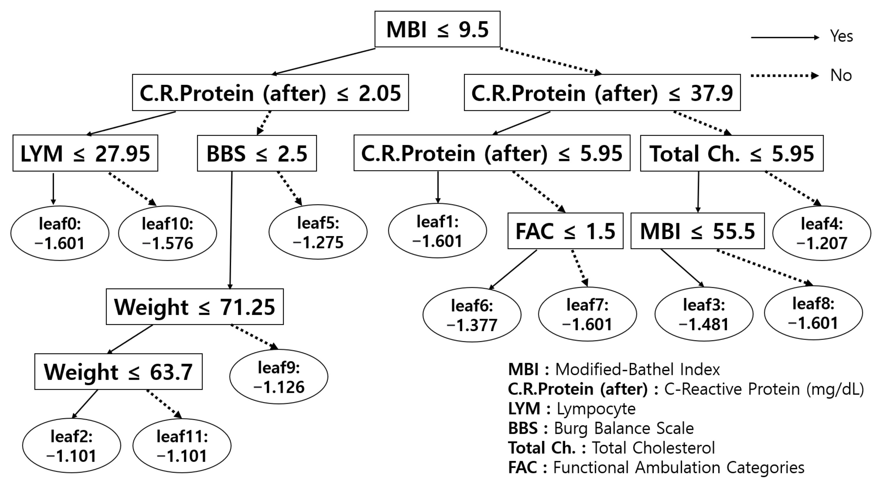
- Decision Tree (DT): although there are many other tree-based ML algorithms, such as ID3 [43] and C4.5 [44], scikit-learn [23,24] uses the classification and regression trees (CART) [45] algorithm. CART is a binary tree classifier where nodes are split into two child nodes repeatedly with Gini’s impurity index as a splitting criterion. With training data, the decision tree is structured in the direction that reduces Gini’s index.
- Perceptron (PT): PT [46,47] is one of the linear discriminant models for binary classification. The input vector x is transformed by a nonlinear transformation to output a feature vector . Then, it is used to construct the following linear model:where is a nonlinear activation function and where target values 1 and −1 correspond to classes 0 and 1, respectively. Then, the stochastic gradient descent algorithm is applied to the perceptron criterion error function to learn the optimal parameter w.
- Light Gradient Boosting Machine (LightGBM): LightGBM [27] is a tree-based ML algorithm that utilizes a gradient boosting framework. It is a gradient-based decision tree (GBDT) with two newly proposed techniques to advance the accuracy and efficiency of GBDT (gradient-based one-sided sampling and exclusive feature bundling). With these components, it successfully deals with a large amount of data instances and features efficiently. It grows its nodes in a leaf-wise manner by selecting nodes that decrease loss. This procedure is different from other tree-based ML algorithms, such as GBT [48], GBDT [49], GBM [50], MART [51], and RF [35].
- Automated machine learning (AutoML): AutoML is proposed to automate ML processes such as data preprocessing, algorithm learning, hyperparameter tuning, and evaluation to apply ML to real-world problems. There are two issues regarding AutoML: combined algorithm selection and hyperparameter optimization (CASH) [52], and neural architecture search (NAS) [53]. Between them, we focused on the CASH problem to find the optimal (best-fitted) algorithms for the data collected and drew similarities between the chosen models and the diagnostician’s prescription process in the real world. Although numerous developed AutoML packages exist, we utilized the latest and best performing AutoGluon [29] library package.
- SuperTML: proposed by Sun et al. [30], SuperTML suggested a new way to deal with classification problems using tabular data with deep neural networks by embedding each instance’s features into a two-dimensional image. It then uses a pretrained convolutional neural network (CNN) [54], consisting of residual networks (ResNet) [2], to extract a representation of the images, after which fully connected layers (with two hidden layers) classify the input. It also automatically handles the categorical and missing values without any preprocessing.
- TabNet: similar to tree-based ML algorithms, Arik and Pfister [31] designed a new deep neural network model that performs similarly to the way the tree-based models perform for tabular data (named as TabNet). While the tree-based algorithms efficiently select global features with information gain [26], TabNet also calculates the weights of each instance’s features via step operation. In the step operation, an attentive transformer outputs a mask that is used to take an element-wise product with each batch-sized instance to calculate a sequence of the feature importance. This process belongs to TabNet’s encoder. Although TabNet also has a decoder, it is for unsupervised learning only. That is why we used only the encoder part for supervised learning with six-step operations.
Appendix B. Formulations of Measurements: Accuracy, Precision, Recall, F1-Score, and Balanced Accuracy
- Notations: K: number of classes, which is 8 in this paper. : number of observations of class i. : true positive of class i. : true negative of class i. : false positive of class i. : false negative of class i.
- Accuracy:
- Balanced accuracy:
- Weighted Precision: ,where
- Weighted recall: ,where
- Weighted F1-score: ,where
Appendix C. Details of the Data

| Numeric Variables | |||
|---|---|---|---|
| Anthropometry | Mean | SD | Range |
| Height (cm) | 165.20 | 8.26 | 140–190 |
| Weight (kg) | 63.19 | 14.62 | 0–120 |
| Stroke | Mean | SD | Range |
| National Institute of Health Stroke Scale (NIHSS) initial (h) | 0.99 | 3.99 | 0–35 |
| NIHSS-tf (h) | 0.42 | 2.47 | 0–20 |
| Blood Test | Mean | SD | Range |
| Hemoglobin (Hb) (g/dL) | 11.87 | 3.57 | 0–38 |
| White Blood Cell (WBC) (/mL) | 6.29 | 3.02 | 0–40 |
| Lymphocytes (LYM%) (%) | 25.93 | 13.00 | 0–57 |
| Iymphocyte count (/mL) | 1.42 | 0.94 | 0–4.88 |
| Glucose (mg/dL) | 95.03 | 46.40 | 0–356 |
| C-reactive Protein (before) (mg/L) | 4.66 | 12.49 | 0–111.38 |
| C-reactive Protein (after) (mg/dL) | 40.08 | 118.82 | 0–1114 |
| Protein (g/dL) | 5.90 | 2.12 | 0–8.4 |
| Albumin (g/dL) | 3.35 | 1.14 | 0–5 |
| Total cholesterol (mg/dL) | 76.15 | 75.04 | 0–288 |
| Functional Assessment | Mean | SD | Range |
| Modified-bathel index (MBI) | 40.90 | 29.80 | 0–100 |
| Mini-mental state examination (MMSE) | 17.29 | 15.65 | 0–330 |
| Modified-ranking scale (mRS) | 1.06 | 1.71 | 0–5 |
| Burg balance scale (BBS) | 20.67 | 18.04 | 0–56 |
| NIHSS | 0.48 | 4.15 | 0–99 |
| Biosignal Ward (Daily Average) | Mean | SD | Range |
| Systolic BP (SBP) | 120.22 | 12.00 | 89–165 |
| Diastolic BP (DBP) | 75.39 | 10.75 | 10–120 |
| Heart rate (HR) | 77.34 | 11.06 | 0–122 |
| Respiratory rate (RR) | 19.03 | 2.03 | 0–28 |
| Categorical Variables | |||||
|---|---|---|---|---|---|
| Disease | |||||
| Comorbidities | |||||
| Diabetes Mellitus (DM) | # | % | Chronic Liver Ds. | # | % |
| Yes | 533 | 33 | Yes | 28 | 1.7 |
| No | 1090 | 67 | No | 1587 | 97.8 |
| Unknown | 0 | 0 | Unknown | 8 | 0.5 |
| Hypertension (HTN) | # | % | Heart Disease | # | % |
| Yes | 1140 | 70 | Yes | 248 | 15.3 |
| No | 483 | 30 | No | 1367 | 84.2 |
| Unknown | 0 | 0 | Unknown | 8 | 0.5 |
| Chronic Kidney ds. (CKD) | # | % | Hyper Lipidemia | # | % |
| Yes | 45 | 2.94 | Yes | 252 | 15.5 |
| No | 1577 | 97 | No | 1368 | 84.3 |
| Unknown | 1 | 0.06 | Unknown | 3 | 0.2 |
| Chronic Lung ds. | # | % | |||
| Yes | 32 | 2 | |||
| No | 1583 | 97.5 | |||
| Unknown | 8 | 0.5 | |||
| Associated Impairment | |||||
| Aphasia | # | % | Neglect | # | % |
| Yes | 493 | 30 | Yes | 313 | 19 |
| No | 971 | 60 | No | 1229 | 76 |
| Unknown | 159 | 10 | Unknown | 81 | 5 |
| Sensory impairment (light-touch) | # | % | Sensory impairment (pin-prick) | # | % |
| Intact | 547 | 34 | Intact | 553 | 34 |
| Impaired | 703 | 43 | Impaired | 694 | 43 |
| Unknown | 373 | 23 | Unknown | 376 | 23 |
| Sensory impairment (proprioception) | # | % | Neuropathic pain | # | % |
| Intact | 508 | 31 | Yes | 68 | 4 |
| Impaired | 684 | 42 | No | 1162 | 72 |
| Unknown | 431 | 27 | Unknown | 393 | 24 |
| Stroke | |||||
|---|---|---|---|---|---|
| Basic Information | |||||
| First or Recurred | # | % | Type of stroke | # | % |
| First-ever Stroke | 1492 | 92 | Ischemic | 693 | 42.7 |
| Recurred stroke | 131 | 8 | Hemorrhagic | 770 | 47.5 |
| Unknown | 0 | 0 | Others | 151 | 9.3 |
| Unknown | 9 | 0.5 | |||
| Acute treatment | # | % | First Hospital | # | % |
| Endovascular Intervention | 80 | 5 | Senior General Hospital | 5 | 0.3 |
| Thrombolysis (IA or IV) | 111 | 7 | General Hospital | 826 | 50.9 |
| Surgery (burrhole or extraventricular drainage WO craniectomy) | 154 | 9 | Hospital | 681 | 42.0 |
| Surgery including craiectomy | 324 | 20 | Oriental Medicine Hospital | 97 | 6.0 |
| Medical Treatment | 885 | 55 | Others | 2 | 0.1 |
| Others | 34 | 2 | Unknown | 12 | 0.7 |
| Unknown | 35 | 2 | |||
| Middle cerebral artery (MCA) | # | % | Anterior cerebral artery (ACA) | # | % |
| Yes | 464 | 28.5 | Yes | 97 | 6 |
| No | 1149 | 71 | No | 1516 | 93.4 |
| Unknown | 10 | 0.6 | Unknown | 10 | 0.6 |
| Posterior Cerebral Artery (PCA) | # | % | Posterior Inferior Cerebellar Artery (PICA) | # | % |
| Yes | 49 | 3 | Yes | 146 | 9 |
| No | 1564 | 96.4 | No | 1467 | 90.4 |
| Unknown | 10 | 0.6 | Unknown | 10 | 0.6 |
| Anterior Inferior Cerebellar Artery (AICA) | # | % | Corona Radiate | # | % |
| Yes | 55 | 3.4 | Yes | 82 | 5 |
| No | 1558 | 96 | No | 1531 | 94.4 |
| Unknown | 10 | 0.6 | Unknown | 10 | 0.6 |
| Others | # | % | |||
| Yes | 409 | 25.2 | |||
| No | 1204 | 74.2 | |||
| Unknown | 10 | 0.6 | |||
| Lesion Location (Hemorrhagic) | |||||
|---|---|---|---|---|---|
| Frontal | # | % | Temporal | # | % |
| Yes | 128 | 8 | Yes | 181 | 11 |
| No | 1495 | 92 | No | 1442 | 89 |
| Unknown | 0 | 0 | Unknown | 0 | 0 |
| Parietal | # | % | Occipital | # | % |
| Yes | 97 | 6 | Yes | 47 | 3 |
| No | 1526 | 94 | No | 1576 | 97 |
| Unknown | 0 | 0 | Unknown | 0 | 0 |
| Basal ganglia | # | % | Brain stem | # | % |
| Yes | 267 | 16.5 | Yes | 73 | 4.5 |
| No | 1356 | 83.5 | No | 1550 | 95.5 |
| Unknown | 0 | 0 | Unknown | 0 | 0 |
| Intracerebral Hemorrhage (ICH) | # | % | Subarachnoid Hemorrhage (SAH) | # | % |
| Yes | 629 | 39 | Yes | 187 | 11.5 |
| No | 994 | 61 | No | 1436 | 88.5 |
| Unknown | 0 | 0 | Unknown | 0 | 0 |
| Subdural Hematoma (SDH) | # | % | Intraventricular Hemorrhage (IVH) | # | % |
| Yes | 84 | 5 | Yes | 233 | 14 |
| No | 1539 | 95 | No | 1390 | 86 |
| Unknown | 0 | 0 | Unknown | 0 | 0 |
| Others | # | % | |||
| Yes | 213 | 13 | |||
| No | 1410 | 87 | |||
| Functional Assessment | |||||
|---|---|---|---|---|---|
| Range of Motion | |||||
| Right Hip | # | % | Left Hip | # | % |
| Full | 1066 | 65.7 | Full | 996 | 61.4 |
| Limited range in flexion | 404 | 24.9 | Limited range in flexion | 478 | 29.5 |
| Limited range in extension | 10 | 0.6 | Limited range in extension | 8 | 0.5 |
| Limited range in both directions | 124 | 7.7 | Limited range in both directions | 122 | 7.5 |
| Unknown | 19 | 1.1 | Unknown | 19 | 1.1 |
| Right Knee | # | % | Left Knee | # | % |
| Full | 1482 | 91.5 | Full | 1472 | 90.7 |
| Limited range in flexion | 106 | 6.5 | Limited range in flexion | 113 | 7 |
| Limited range in extension | 4 | 0.2 | Limited range in extension | 7 | 0.45 |
| Limited range in both directions | 12 | 0.7 | Limited range in both directions | 12 | 0.75 |
| Unknown | 19 | 1.1 | Unknown | 19 | 1.1 |
| Right Ankle | # | % | Left Ankle | # | % |
| Full | 1088 | 67.1 | Full | 1198 | 73.8 |
| Limited range in flexion | 436 | 26.8 | Limited range in flexion | 315 | 19.4 |
| Limited range in extension | 16 | 1 | Limited range in extension | 17 | 1.1 |
| Limited range in both directions | 64 | 4 | Limited range in both directions | 74 | 4.6 |
| Unknown | 19 | 1.1 | Unknown | 19 | 1.1 |
| Modified Ashworth Scale | |||||
| Right Elbow Flexor | # | % | Left Elbow Flexor | # | % |
| 0 grade | 1389 | 85.6 | 0 grade | 1285 | 79.1 |
| 1 grade | 111 | 6.8 | 1 grade | 181 | 11.14 |
| 2 grade | 105 | 6.5 | 2 grade | 115 | 7.1 |
| 3 grade | 4 | 0.2 | 3 grade | 27 | 1.7 |
| 4 grade | 0 | 0 | 4 grade | 1 | 0.06 |
| Unknown | 14 | 0.9 | Unknown | 14 | 0.9 |
| Right Knee Flexor | # | % | Left Knee Flexor | # | % |
| 0 grade | 1366 | 84.2 | 0 grade | 1268 | 78.1 |
| 1 grade | 177 | 10.8 | 1 grade | 236 | 14.5 |
| 2 grade | 47 | 2.9 | 2 grade | 82 | 5.1 |
| 3 grade | 19 | 1.2 | 3 grade | 23 | 1.4 |
| 4 grade | 0 | 0 | 4 grade | 0 | 0 |
| Unknown | 14 | 0.9 | Unknown | 14 | 0.9 |
| Manual Muscle Test | |||||
|---|---|---|---|---|---|
| Right Hip Flexor | # | % | Left Hip Flexor | # | % |
| Zero | 97 | 6 | Zero | 88 | 5.4 |
| Trace | 169 | 10.4 | Trace | 126 | 7.8 |
| Poor | 302 | 18.6 | Poor | 204 | 12.6 |
| Fair | 340 | 20.9 | Fair | 303 | 18.6 |
| Good | 510 | 31.4 | Good | 524 | 32.3 |
| Normal | 186 | 11.5 | Normal | 359 | 22.1 |
| Unknown | 19 | 1.2 | Unknown | 19 | 1.2 |
| Right Knee Extensor | # | % | Left Knee Extensor | # | % |
| Zero | 99 | 6.1 | Zero | 94 | 5.8 |
| Trace | 229 | 14.1 | Trace | 133 | 8.2 |
| Poor | 231 | 14.2 | Poor | 190 | 11.7 |
| Fair | 331 | 20.4 | Fair | 294 | 18.1 |
| Good | 522 | 32.2 | Good | 533 | 32.8 |
| Normal | 190 | 11.7 | Normal | 360 | 22.2 |
| Unknown | 21 | 1.3 | Unknown | 19 | 1.2 |
| Right Dorsi Flexor | # | % | Left Dorsi Flexor | # | % |
| Zero | 110 | 6.8 | Zero | 120 | 7.4 |
| Trace | 314 | 19.3 | Trace | 300 | 18.5 |
| Poor | 280 | 17.3 | Poor | 129 | 7.9 |
| Fair | 200 | 12.3 | Fair | 185 | 11.4 |
| Good | 510 | 31.5 | Good | 517 | 31.9 |
| Normal | 188 | 11.6 | Normal | 353 | 21.7 |
| Unknown | 21 | 1.2 | Unknown | 19 | 1.2 |
| Functional Ambulation Category (FAC) | # | % | |||
| Total Assist | 394 | 24.3 | |||
| Maximal Moderate Assist | 490 | 30.2 | |||
| Minimal Assist | 236 | 14.5 | |||
| Supervision | 279 | 17.2 | |||
| Partly Independent | 147 | 9.1 | |||
| Fully Independent | 56 | 3.4 | |||
| Unknown | 21 | 1.3 | |||
References
- Bornstein, B.H.; Emler, A.C. Rationality in medical decision making: A review of the literature on doctors’ decision-making biases. J. Eval. Clin. Pract. 2001, 7, 97–107. [Google Scholar] [CrossRef]
- He, K.; Zhang, X.; Ren, S.; Sun, J. Deep residual learning for image recognition. In Proceedings of the IEEE Conference on Computer Vision and Pattern Recognition, Las Vegas, NV, USA, 27–30 June 2016; pp. 770–778. [Google Scholar]
- Simonyan, K.; Zisserman, A. Very deep convolutional networks for large-scale image recognition. arXiv 2014, arXiv:1409.1556. [Google Scholar]
- Silver, D.; Schrittwieser, J.; Simonyan, K.; Antonoglou, I.; Huang, A.; Guez, A.; Hubert, T.; Baker, L.; Lai, M.; Bolton, A.; et al. Mastering the game of go without human knowledge. Nature 2017, 550, 354–359. [Google Scholar] [CrossRef]
- Mnih, V.; Kavukcuoglu, K.; Silver, D.; Graves, A.; Antonoglou, I.; Wierstra, D.; Riedmiller, M. Playing atari with deep reinforcement learning. arXiv 2013, arXiv:1312.5602. [Google Scholar]
- Vinyals, O.; Babuschkin, I.; Czarnecki, W.M.; Mathieu, M.; Dudzik, A.; Chung, J.; Choi, D.H.; Powell, R.; Ewalds, T.; Georgiev, P.; et al. Grandmaster level in StarCraft II using multi-agent reinforcement learning. Nature 2019, 575, 350–354. [Google Scholar] [CrossRef] [PubMed]
- Charan, S.; Khan, M.J.; Khurshid, K. Breast cancer detection in mammograms using convolutional neural network. In Proceedings of the 2018 International Conference on Computing, Mathematics and Engineering Technologies (iCoMET), Sukkur, Pakistan, 3–4 March 2018; pp. 1–5. [Google Scholar]
- Mathe, J.; Werner, J.; Lee, Y.; Malin, B.; Ledeczi, A. Model-based design of clinical information systems. Methods Inf. Med. 2008, 47, 399. [Google Scholar]
- Abedi, V.; Goyal, N.; Tsivgoulis, G.; Hosseinichimeh, N.; Hontecillas, R.; Bassaganya-Riera, J.; Elijovich, L.; Metter, J.E.; Alexandrov, A.W.; Liebeskind, D.S.; et al. Novel screening tool for stroke using artificial neural network. Stroke 2017, 48, 1678–1681. [Google Scholar] [CrossRef] [PubMed]
- Park, S.J.; Hussain, I.; Hong, S.; Kim, D.; Park, H.; Benjamin, H.C.M. Real-time Gait Monitoring System for Consumer Stroke Prediction Service. In Proceedings of the 2020 IEEE International Conference on Consumer Electronics (ICCE), Las Vegas, NV, USA, 4–6 January 2020; pp. 1–4. [Google Scholar]
- Wei, X.; Zhang, X.; Yi, P. Design of control system for elderly-assistant & walking-assistant robot based on fuzzy adaptive method. In Proceedings of the 2012 IEEE International Conference on Mechatronics and Automation, Chengdu, China, 5–8 August 2012; pp. 2083–2087. [Google Scholar]
- Lozano-Quilis, J.A.; Gil-Gomez, H.; Gil-Gómez, J.A.; Albiol-Perez, S.; Palacios, G.; Fardoum, H.M.; Mashat, A.S. Virtual reality system for multiple sclerosis rehabilitation using KINECT. In Proceedings of the 2013 7th International Conference on Pervasive Computing Technologies for Healthcare and Workshops, Venice, Italy, 5–8 May 2013; pp. 366–369. [Google Scholar]
- Scrutinio, D.; Ricciardi, C.; Donisi, L.; Losavio, E.; Battista, P.; Guida, P.; Cesarelli, M.; Pagano, G.; D’Addio, G. Machine learning to predict mortality after rehabilitation among patients with severe stroke. Sci. Rep. 2020, 10, 1–10. [Google Scholar] [CrossRef]
- Mannini, A.; Trojaniello, D.; Cereatti, A.; Sabatini, A.M. A machine learning framework for gait classification using inertial sensors: Application to elderly, post-stroke and huntington’s disease patients. Sensors 2016, 16, 134. [Google Scholar] [CrossRef] [PubMed]
- Harari, Y.; O’Brien, M.K.; Lieber, R.L.; Jayaraman, A. Inpatient stroke rehabilitation: Prediction of clinical outcomes using a machine-learning approach. J. Neuroeng. Rehabil. 2020, 17, 1–10. [Google Scholar] [CrossRef] [PubMed]
- Cristianini, N.; Ricci, E. Support Vector Machines. In Encyclopedia of Algorithms; Kao, M.Y., Ed.; Springer: Boston, MA, USA, 2008; pp. 928–932. [Google Scholar] [CrossRef]
- Rabiner, L.; Juang, B. An introduction to hidden Markov models. IEEE Assp Mag. 1986, 3, 4–16. [Google Scholar] [CrossRef]
- Tibshirani, R. Regression shrinkage and selection via the lasso. J. R. Stat. Soc. Ser. B Methodol. 1996, 58, 267–288. [Google Scholar] [CrossRef]
- Chawla, N.V.; Bowyer, K.W.; Hall, L.O.; Kegelmeyer, W.P. SMOTE: Synthetic minority over-sampling technique. J. Artif. Intell. Res. 2002, 16, 321–357. [Google Scholar] [CrossRef]
- Tomek, I. Two Modifications of CNN. IEEE Trans. Syst. Man Cybern. 1976, SMC-6, 769–772. [Google Scholar] [CrossRef]
- Batista, G.E.; Prati, R.C.; Monard, M.C. A study of the behavior of several methods for balancing machine learning training data. ACM SIGKDD Explor. Newsl. 2004, 6, 20–29. [Google Scholar] [CrossRef]
- Lemaître, G.; Nogueira, F.; Aridas, C.K. Imbalanced-learn: A Python Toolbox to Tackle the Curse of Imbalanced Datasets in Machine Learning. J. Mach. Learn. Res. 2017, 18, 1–5. [Google Scholar]
- Pedregosa, F.; Varoquaux, G.; Gramfort, A.; Michel, V.; Thirion, B.; Grisel, O.; Blondel, M.; Prettenhofer, P.; Weiss, R.; Dubourg, V.; et al. Scikit-learn: Machine Learning in Python. J. Mach. Learn. Res. 2011, 12, 2825–2830. [Google Scholar]
- Buitinck, L.; Louppe, G.; Blondel, M.; Pedregosa, F.; Mueller, A.; Grisel, O.; Niculae, V.; Prettenhofer, P.; Gramfort, A.; Grobler, J.; et al. API design for machine learning software: Experiences from the scikit-learn project. arXiv 2013, arXiv:1309.0238. [Google Scholar]
- Gallant, S.I. Perceptron-based learning algorithms. IEEE Trans. Neural Netw. 1990, 1, 179–191. [Google Scholar] [CrossRef]
- Safavian, S.R.; Landgrebe, D. A survey of decision tree classifier methodology. IEEE Trans. Syst. Man Cybern. 1991, 21, 660–674. [Google Scholar] [CrossRef]
- Ke, G.; Meng, Q.; Finley, T.; Wang, T.; Chen, W.; Ma, W.; Ye, Q.; Liu, T.Y. Lightgbm: A highly efficient gradient boosting decision tree. Adv. Neural Inf. Process. Syst. 2017, 30, 3146–3154. [Google Scholar]
- He, X.; Zhao, K.; Chu, X. AutoML: A Survey of the State-of-the-Art. Knowl. Based Syst. 2019, 212, 106622. [Google Scholar] [CrossRef]
- Erickson, N.; Mueller, J.; Shirkov, A.; Zhang, H.; Larroy, P.; Li, M.; Smola, A. AutoGluon-Tabular: Robust and Accurate AutoML for Structured Data. arXiv 2020, arXiv:2003.06505. [Google Scholar]
- Sun, B.; Yang, L.; Zhang, W.; Lin, M.; Dong, P.; Young, C.; Dong, J. Supertml: Two-dimensional word embedding for the precognition on structured tabular data. In Proceedings of the IEEE/CVF Conference on Computer Vision and Pattern Recognition Workshops, Long Beach, CA, USA, 16–17 June 2019; pp. 2973–2981. [Google Scholar]
- Arik, S.O.; Pfister, T. Tabnet: Attentive interpretable tabular learning. arXiv 2019, arXiv:1908.07442. [Google Scholar]
- Murphy, K.P. Machine Learning: A Probabilistic Perspective; MIT Press: Cambridge, MA, USA, 2012. [Google Scholar]
- Schmarje, L.; Santarossa, M.; Schröder, S.M.; Koch, R. A survey on semi-, self-and unsupervised techniques in image classification. arXiv 2020, arXiv:2002.08721. [Google Scholar]
- Dorogush, A.V.; Ershov, V.; Gulin, A. CatBoost: Gradient boosting with categorical features support. arXiv 2018, arXiv:1810.11363. [Google Scholar]
- Ho, T.K. Random decision forests. In Proceedings of the 3rd International Conference on Document Analysis and Recognition, Montreal, QC, Canada, 14–16 August 1995; Volume 1, pp. 278–282. [Google Scholar]
- Geurts, P.; Ernst, D.; Wehenkel, L. Extremely randomized trees. Mach. Learn. 2006, 63, 3–42. [Google Scholar] [CrossRef]
- Karthiga, A.S.; Mary, M.S.; Yogasini, M. Early prediction of heart disease using decision tree algorithm. Int. J. Adv. Res. Basic Eng. Sci. Technol. 2017, 3, 1–16. [Google Scholar]
- Kassirer, J.P.; Gorry, G.A. Clinical problem solving: A behavioral analysis. Ann. Intern. Med. 1978, 89, 245–255. [Google Scholar] [CrossRef] [PubMed]
- Gruppen, L.D.; Palchik, N.S.; Wolf, F.M.; Laing, T.J.; Oh, M.S.; Davis, W.K. Medical student use of history and physical information in diagnostic reasoning. Arthritis Rheum. J. Am. Coll. Rheumatol. 1993, 6, 64–70. [Google Scholar] [CrossRef]
- Brush Jr, J.E.; Sherbino, J.; Norman, G.R. How expert clinicians intuitively recognize a medical diagnosis. Am. J. Med. 2017, 130, 629–634. [Google Scholar] [CrossRef]
- Middleton, K.; Butt, M.; Hammerla, N.; Hamblin, S.; Mehta, K.; Parsa, A. Sorting out symptoms: Design and evaluation of the’babylon check’automated triage system. arXiv 2016, arXiv:1606.02041. [Google Scholar]
- Cortes, C.; Vapnik, V. Support-vector networks. Mach. Learn. 1995, 20, 273–297. [Google Scholar] [CrossRef]
- Quinlan, J.R. Induction of decision trees. Mach. Learn. 1986, 1, 81–106. [Google Scholar] [CrossRef]
- Quinlan, J.R. C4.5: Programs for Machine Learning; Elsevier: Amsterdam, The Netherlands, 2014. [Google Scholar]
- Breiman, L.; Friedman, J.; Stone, C.J.; Olshen, R.A. Classification and Regression Trees; CRC Press: Boca Raton, FL, USA, 1984. [Google Scholar]
- Rosenblatt, F. The perceptron: A probabilistic model for information storage and organization in the brain. Psychol. Rev. 1958, 65, 386. [Google Scholar] [CrossRef] [PubMed]
- Bishop, C.M. Pattern Recognition and Machine Learning; Springer: Berlin/Heidelberg, Germany, 2006. [Google Scholar]
- Friedman, J.H. Stochastic gradient boosting. Comput. Stat. Data Anal. 2002, 38, 367–378. [Google Scholar] [CrossRef]
- Hastie, T.; Tibshirani, R.; Friedman, J. Boosting and additive trees. In The Elements of Statistical Learning; Springer: Berlin/Heidelberg, Germany, 2009; pp. 337–387. [Google Scholar]
- Ridgeway, G. Generalized Boosted Models: A guide to the gbm package. Update 2007, 1, 2007. [Google Scholar]
- Friedman, J.H.; Meulman, J.J. Multiple additive regression trees with application in epidemiology. Stat. Med. 2003, 22, 1365–1381. [Google Scholar] [CrossRef]
- Thornton, C.; Hutter, F.; Hoos, H.H.; Leyton-Brown, K. Auto-WEKA: Combined selection and hyperparameter optimization of classification algorithms. In Proceedings of the 19th ACM SIGKDD International Conference on Knowledge Discovery and Data Mining, Chicago, lL, USA, 11–14 August 2013; pp. 847–855. [Google Scholar]
- Elsken, T.; Metzen, J.H.; Hutter, F. Neural architecture search: A survey. J. Mach. Learn. Res. 2019, 20, 1–21. [Google Scholar]
- Simard, P.Y.; Steinkraus, D.; Platt, J.C. Best practices for convolutional neural networks applied to visual document analysis. In Proceedings of the Seventh International Conference on Document Analysis and Recognition, Edinburgh, Scotland, 3–6 August 2003; Volume 2, pp. 958–962. [Google Scholar]


| CAUH | SNUH | NTIRH | CUYMH | AMC e | |
|---|---|---|---|---|---|
| The number of patients | 29 | 7 | 132 | 173 | 42 |
| The number of observations | 85 | 34 | 691 | 571 | 242 |
| Original Data | |||||
|---|---|---|---|---|---|
| ML/DL Models | Accuracy (%) | Recall (%) | Precision (%) | F1-Score (%) | Balanced Accuracy (%) |
| SVM | 52.1 ± 1.5 | 52.1 ± 1.5 | 53.8 ± 2.5 | 50.4 ± 1.5 | 41.8 ± 1.5 |
| DecisionTree | 86.0 ± 1.0 | 86.0 ± 1.0 | 86.4 ± 1.1 | 86.0 ± 1.1 | 79.0 ± 1.9 |
| Perceptron | 39.1 ± 3.2 | 39.1 ± 3.2 | 64.3 ± 2.8 | 34.7 ± 3.7 | 32.3 ± 2.6 |
| LightGBM | 91.2 ± 0.5 | 91.2 ± 0.5 | 91.5 ± 0.5 | 91.1 ± 0.5 | 85.8 ± 1.4 |
| AutoGluon | 91.7 ± 0.3 | 91.7 ± 0.3 | 92.0 ± 0.3 | 91.7 ± 0.3 | 86.8 ± 1.3 |
| SuperTML | 89.3 ± 0.8 | 89.3 ± 0.8 | 89.8 ± 0.8 | 89.2 ± 0.9 | 83.1 ± 2.4 |
| TabNet | 89.5 ± 0.6 | 89.5 ± 0.6 | 89.8 ± 0.6 | 89.4 ± 0.6 | 84.0 ± 1.4 |
| SMOTE (Over Sampling) | |||||
| ML/DL Models | Accuracy (%) | Recall (%) | Precision (%) | F1-Score (%) | Balanced Accuracy (%) |
| SVM | 57.7 ± 1.6 | 57.7 ± 1.6 | 63.9 ± 2.1 | 59.7 ± 1.8 | 52.5 ± 3.1 |
| DecisionTree | 86.1 ± 0.7 | 86.1 ± 0.7 | 86.6 ± 0.7 | 86.1 ± 0.7 | 80.7 ± 2.5 |
| Perceptron | 38.2 ± 3.6 | 38.2 ± 3.6 | 62.7 ± 2.9 | 35.1 ± 3.6 | 32.9 ± 2.9 |
| LightGBM | 90.8 ± 0.7 | 90.8 ± 0.7 | 91.2 ± 0.6 | 90.8 ± 0.7 | 86.1 ± 1.2 |
| AutoGluon | 91.0 ± 0.2 | 91.0 ± 0.2 | 91.3 ± 0.2 | 90.9 ± 0.2 | 86.6 ± 1.2 |
| SuperTML | 90.3 ± 0.9 | 90.3 ± 0.9 | 90.6 ± 0.9 | 90.2 ± 0.9 | 84.1 ± 1.4 |
| TabNet | 89.5 ± 0.5 | 89.5 ± 0.5 | 90.0 ± 0.5 | 89.5 ± 0.5 | 84.9 ± 1.6 |
| TomekLinks (Under Sampling) | |||||
| ML/DL Models | Accuracy (%) | Recall (%) | Precision (%) | F1-Score (%) | Balanced Accuracy (%) |
| SVM | 53.1 ± 1.6 | 53.1 ± 1.6 | 55.2 ± 1.6 | 51.5 ± 1.8 | 42.4 ± 1.4 |
| DecisionTree | 84.9 ± 0.8 | 84.9 ± 0.8 | 85.5 ± 0.8 | 84.9 ± 0.8 | 78.6 ± 2.3 |
| Perceptron | 35.6 ± 5.7 | 35.6 ± 5.7 | 66.5 ± 4.3 | 32.2 ± 4.3 | 31.0 ± 3.3 |
| LightGBM | 90.0 ± 0.6 | 90.0 ± 0.6 | 90.4 ± 0.6 | 90.0 ± 0.6 | 85.0 ± 2.5 |
| AutoGluon | 90.2 ± 0.2 | 90.2 ± 0.2 | 90.7 ± 0.1 | 90.2 ± 0.2 | 85.9 ± 1.6 |
| SuperTML | 89.0 ± 0.8 | 89.0 ± 0.8 | 89.6 ± 0.8 | 88.9 ± 0.8 | 82.4 ± 1.4 |
| TabNet | 88.4 ± 0.9 | 88.4 ± 0.9 | 88.8 ± 0.8 | 88.4 ± 0.8 | 83.0 ± 1.6 |
| SMOTETomek (Combined Sampling) | |||||
| ML/DL Models | Accuracy (%) | Recall (%) | Precision (%) | F1-Score (%) | Balanced Accuracy (%) |
| SVM | 57.5 ± 1.5 | 57.5 ± 1.5 | 63.7 ± 1.5 | 59.4 ± 1.6 | 52.5 ± 2.7 |
| DecisionTree | 85.7 ± 0.9 | 85.7 ± 0.9 | 86.2 ± 1.0 | 85.8 ± 0.9 | 80.3 ± 2.4 |
| Perceptron | 39.9 ± 3.9 | 39.9 ± 3.9 | 62.5 ± 2.4 | 36.0 ± 4.6 | 34.3 ± 3.8 |
| LightGBM | 90.4 ± 0.7 | 90.4 ± 0.7 | 90.8 ± 0.6 | 90.4 ± 0.6 | 85.8 ± 1.6 |
| AutoGluon | 90.4 ± 0.2 | 90.4 ± 0.2 | 90.7 ± 0.2 | 90.4 ± 0.2 | 85.6 ± 1.4 |
| SuperTML | 89.8 ± 1.4 | 89.8 ± 0.9 | 90.4 ± 0.9 | 89.8 ± 0.9 | 83.3 ± 1.7 |
| TabNet | 89.2 ± 0.8 | 89.2 ± 0.8 | 89.6 ± 0.9 | 89.2 ± 0.8 | 85.3 ± 2.7 |
| Ranking | Model | Score_Test | Score_Val | Stack_Level | Fit_Order |
|---|---|---|---|---|---|
| 1 | CatboostClassifier | −0.196 | −0.299 | 1 | 22 |
| 2 | LightGBMClassifierXT | −0.200 | −0.293 | 1 | 21 |
| 3 | weighted_ensemble | −0.211 | −0.269 | 2 | 24 |
| 4 | LightGBMClassifierCustom | −0.214 | −0.345 | 1 | 23 |
| 5 | LightGBMClassifier | −0.217 | −0.318 | 1 | 20 |
| 6 | RandomForestClassifierEntr | −0.223 | −0.304 | 1 | 17 |
| 7 | ExtraTreesClassifierGini | −0.228 | −0.272 | 1 | 18 |
| 8 | ExtraTreesClassifierEntr | −0.231 | −0.281 | 1 | 19 |
| 9 | weighted_ensemble | −0.236 | −0.319 | 1 | 12 |
| 10 | ExtraTreesClassifierEntr | −0.246 | −0.388 | 0 | 7 |
| 11 | ExtraTreesClassifierGini | −0.249 | −0.380 | 0 | 6 |
| 12 | CatboostClassifier | −0.254 | −0.354 | 0 | 10 |
| 13 | LightGBMClassifierXT | −0.254 | −0.347 | 0 | 9 |
| 14 | LightGBMClassifier | −0.270 | −0.369 | 0 | 8 |
| 15 | LightGBMClassifierCustom | −0.276 | −0.396 | 0 | 11 |
| 16 | RandomForestClassifierGini | −0.278 | −0.305 | 1 | 16 |
| 17 | NeuralNetClassifier | −0.303 | −0.416 | 0 | 1 |
| 18 | RandomForestClassifierEntr | −0.311 | −0.374 | 0 | 5 |
| 19 | NeuralNetClassifier | −0.313 | −0.421 | 1 | 13 |
| 20 | RandomForestClassifierGini | −0.318 | −0.381 | 0 | 4 |
| 21 | KNeighborsClassifierDist | −1.058 | −1.625 | 1 | 15 |
| 22 | KNeighborsClassifierDist | −1.074 | −1.757 | 0 | 3 |
| 23 | KNeighborsClassifierUnif | −1.227 | −1.767 | 1 | 14 |
| 24 | KNeighborsClassifierUnif | −1.269 | −1.901 | 0 | 2 |
Publisher’s Note: MDPI stays neutral with regard to jurisdictional claims in published maps and institutional affiliations. |
© 2021 by the authors. Licensee MDPI, Basel, Switzerland. This article is an open access article distributed under the terms and conditions of the Creative Commons Attribution (CC BY) license (https://creativecommons.org/licenses/by/4.0/).
Share and Cite
Seo, K.; Chung, B.; Panchaseelan, H.P.; Kim, T.; Park, H.; Oh, B.; Chun, M.; Won, S.; Kim, D.; Beom, J.; et al. Forecasting the Walking Assistance Rehabilitation Level of Stroke Patients Using Artificial Intelligence. Diagnostics 2021, 11, 1096. https://doi.org/10.3390/diagnostics11061096
Seo K, Chung B, Panchaseelan HP, Kim T, Park H, Oh B, Chun M, Won S, Kim D, Beom J, et al. Forecasting the Walking Assistance Rehabilitation Level of Stroke Patients Using Artificial Intelligence. Diagnostics. 2021; 11(6):1096. https://doi.org/10.3390/diagnostics11061096
Chicago/Turabian StyleSeo, Kanghyeon, Bokjin Chung, Hamsa Priya Panchaseelan, Taewoo Kim, Hyejung Park, Byungmo Oh, Minho Chun, Sunjae Won, Donkyu Kim, Jaewon Beom, and et al. 2021. "Forecasting the Walking Assistance Rehabilitation Level of Stroke Patients Using Artificial Intelligence" Diagnostics 11, no. 6: 1096. https://doi.org/10.3390/diagnostics11061096
APA StyleSeo, K., Chung, B., Panchaseelan, H. P., Kim, T., Park, H., Oh, B., Chun, M., Won, S., Kim, D., Beom, J., Jeon, D., & Yang, J. (2021). Forecasting the Walking Assistance Rehabilitation Level of Stroke Patients Using Artificial Intelligence. Diagnostics, 11(6), 1096. https://doi.org/10.3390/diagnostics11061096