
MB-AI-His: Histopathological Diagnosis of Pediatric Medulloblastoma and its Subtypes via AI


Abstract
1. Introduction
- Few related studies were conducted for classifying the four subtypes of pediatric MB. Most of them did not achieve very high performance, so they are not reliable. In this paper, a reliable CADx is constructed, called MB-AI-His, that can classify the four subtypes of pediatric MB with high accuracy.
- Most previous studies depend only on textural analysis-based features or deep learning features that were used individually to perform classification; however, MB-AI-His merges the benefits of the DL and textural analysis feature extraction methods through a cascaded manner.
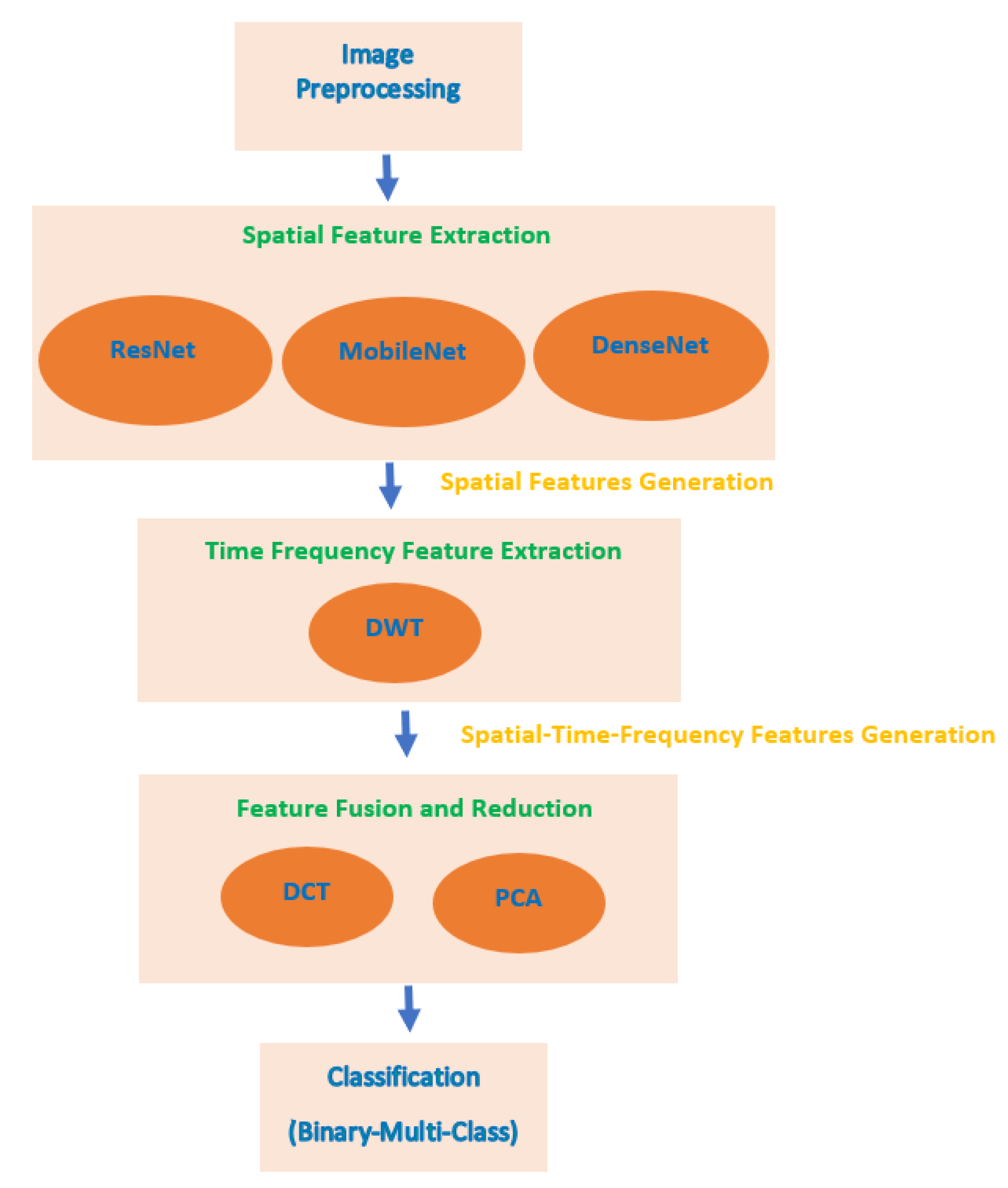
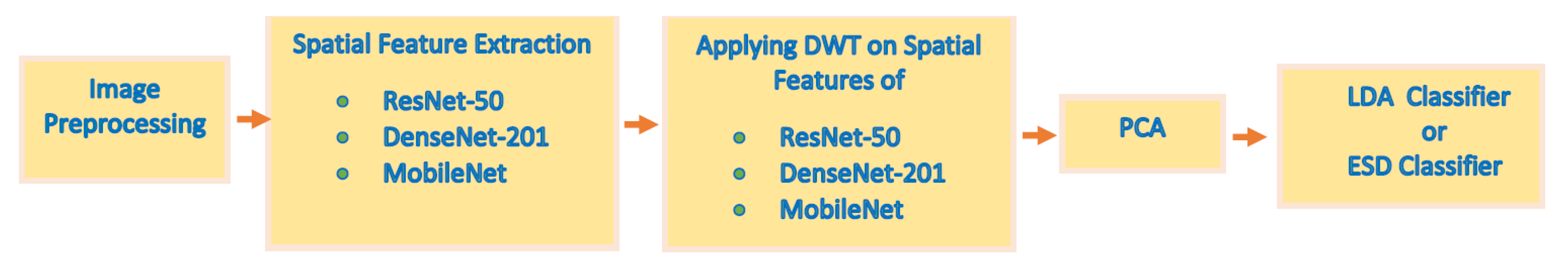
- The cascaded manner initially uses three deep CNNs to extract spatial features. Then, these spatial features enter a DWT which is a textural analysis-based method that generates time-frequency features ending up by generating spatial-time-frequency features.
- Developing spatial-time-frequency features instead of using only spatial features as accomplished by most of the related studies.
- Almost all the related studies used an individual feature set to construct their classification model; however, MB-AI-His fuses the three spatial-time-frequency features generated from the three CNNs and DWT.
- The fusion is done through DCT and PCA to generate a time-efficient CADx system and lower the feature space dimension as well as the classification training time which was one of the limitations in the previous related work.
2. Related Work
3. Materials and Methods
3.1. Childhood MB Dataset Description
3.2. Deep Learning Approaches
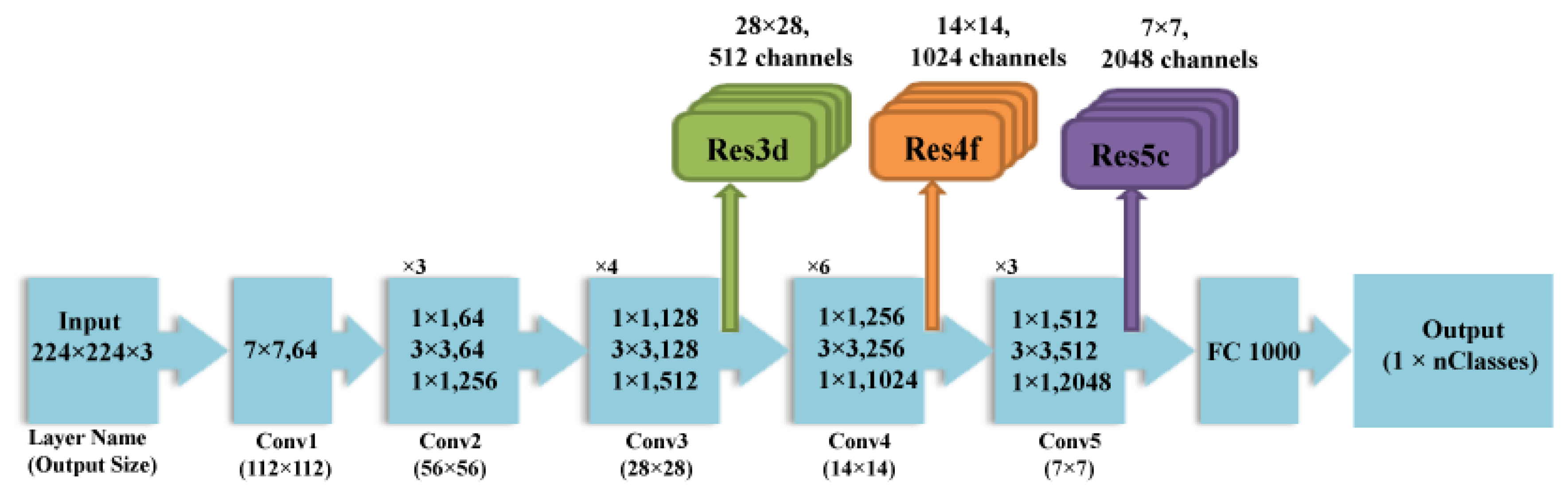
3.2.1. ResNet-50
3.2.2. DenseNet-201
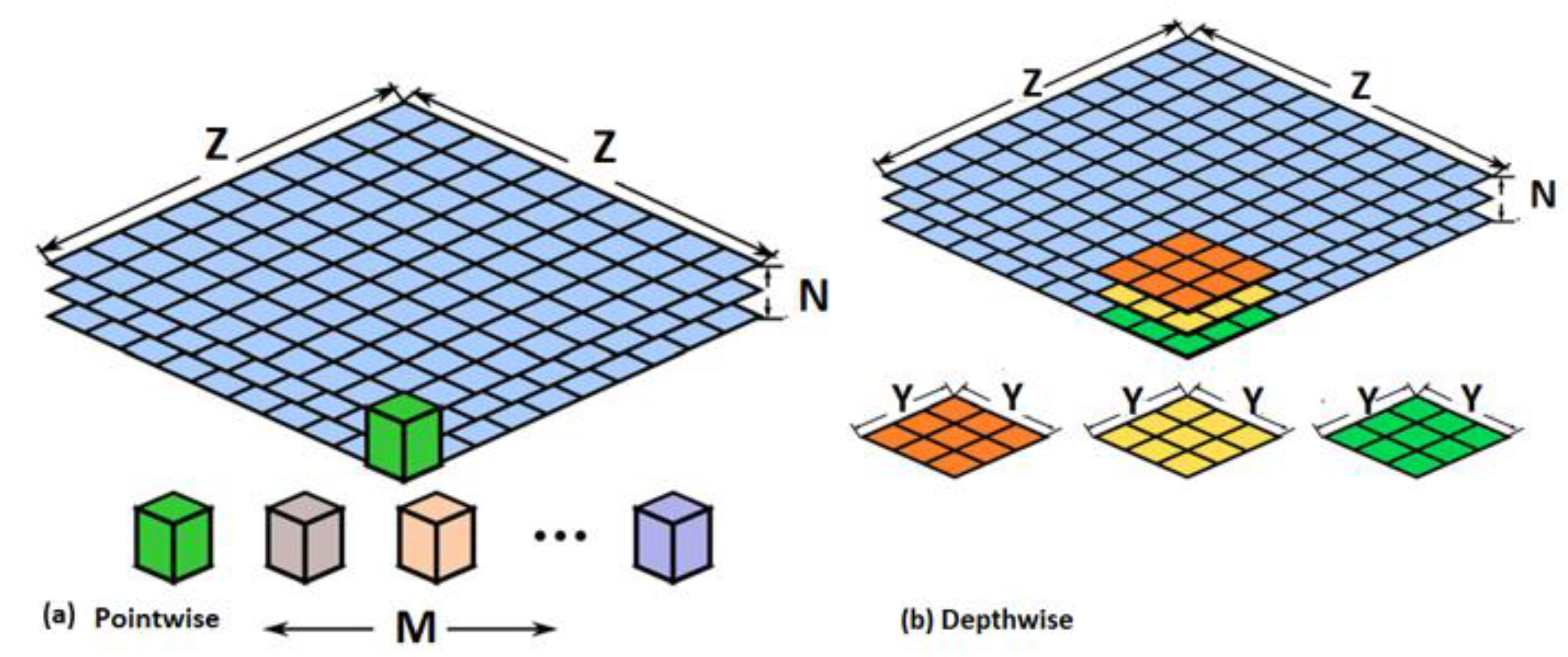
3.2.3. MobileNet
3.3. Proposed MB-AI-His
3.3.1. Image Pre-Processing
3.3.2. Spatial Feature Extraction
3.3.3. Time-Frequency Feature Extraction
3.3.4. Feature Fusion and Reduction
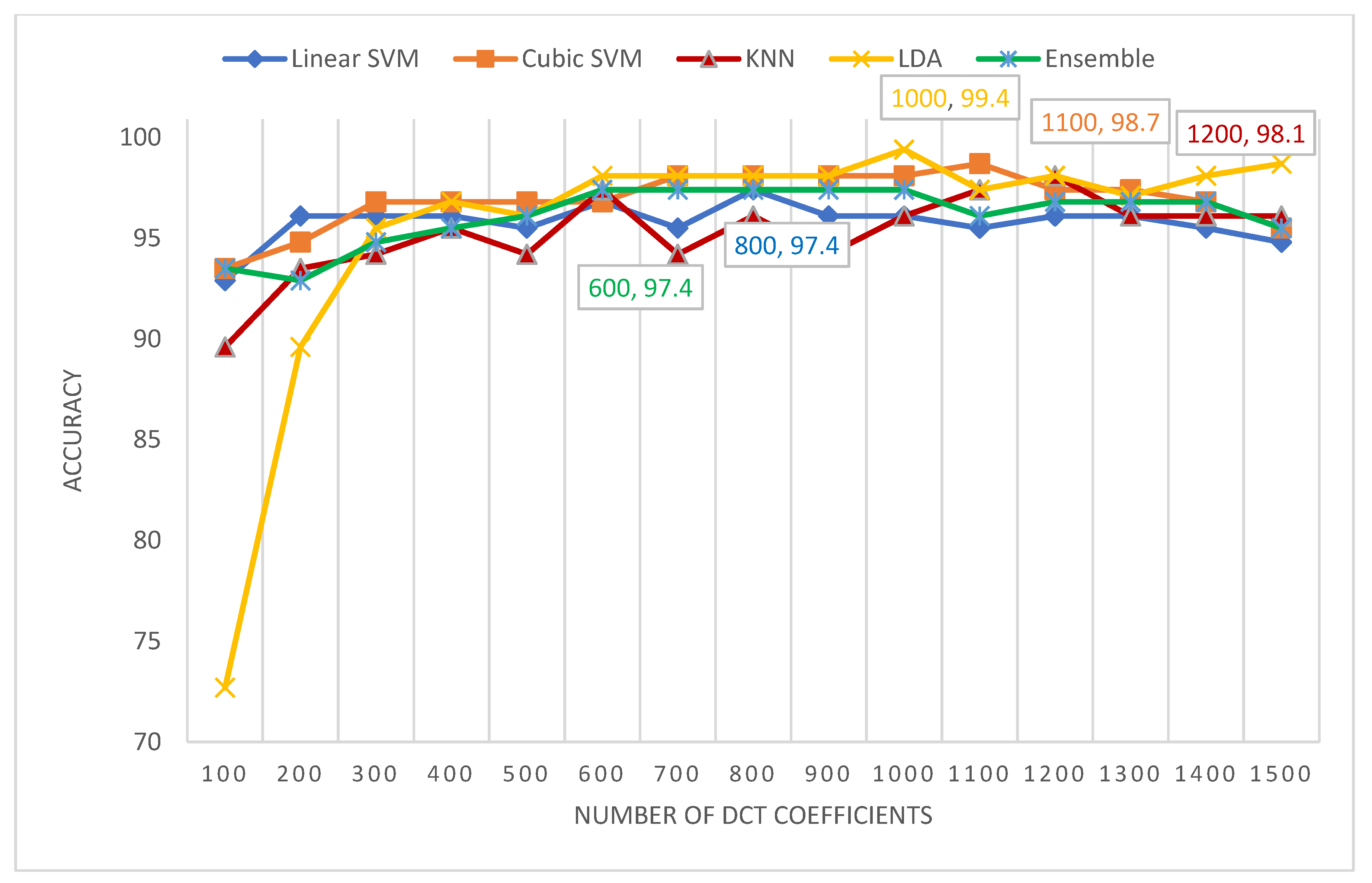
- DCT is regularly applied to decompose a data into primitive frequency elements. It reveals the data as a total of cosine functions fluctuating at separate frequencies [55]. Usually, the DCT is applied to the data to get the DCT coefficients which are split into two groups [56,57]; low frequencies are known as DC coefficients, and high frequencies are known as AC coefficients. High frequencies illustrate edge, details, and tiny changes [57], while low frequencies are linked with the brightness situations. The dimension of the DCT coefficient matrix is identical to the input data [58].
- PCA is a popular feature reduction approach that is commonly employed to compress the huge dimension of features via operating a covariance analysis among observed features. The PCA lessens the full number of observed variables to a reduced quantity of principal components. Such principal components resemble the variance of the original features. It is generally utilized if the observed features of a dataset are very correlated. The PCA is appropriate for datasets having very huge dimensions [59].
3.3.5. Classification
4. Experimental Setup
4.1. Parameters Setting
4.2. Evaluation Metrics
- True Positives (TP): Images that have their true label as positive and whose class is correctly classified to be positive.
- False Positives (FP): Images that have their true label as negative and whose class is wrongly classified to be positive.
- True Negatives (TN): Images that have their true label as negative and whose class is precisely classified to be negative.
- False Negatives (FN): Images that have their true label as positive and whose class is wrongly classified to be negative.
5. Results
5.1. Scenario I Results
5.2. Scenario II Results
5.3. Scenario III Results
5.4. Scenario IV Results
6. Discussion
7. Conclusions
Funding
Institutional Review Board Statement
Informed Consent Statement
Data Availability Statement
Conflicts of Interest
References
- Grist, J.T.; Withey, S.; MacPherson, L.; Oates, A.; Powell, S.; Novak, J.; Abernethy, L.; Pizer, B.; Grundy, R.; Bailey, S. Distin-guishing between Paediatric Brain Tumour Types Using Multi-Parametric Magnetic Resonance Imaging and Machine Learning: A Multi-Site Study. NeuroImage Clin. 2020, 25, 102172. [Google Scholar] [CrossRef] [PubMed]
- Bright, C.; Reulen, R.; Fidler, M.; Guha, J.; Henson, K.; Wong, K.; Kelly, J.; Frobisher, C.; Winter, D.; Hawkins, M. Cerebro-vascular Complications in 208,769 5-Year Survivors of Cancer Diagnosed Aged 15–39 Years Using Hospital Episode Statistics: The Population-Based Teenage and Young Adult Cancer Survivor Study (TYACSS): Abstract O-24. Eur. J. Cancer Care 2015, 24, 9. [Google Scholar]
- Dong, J.; Li, L.; Liang, S.; Zhao, S.; Zhang, B.; Meng, Y.; Zhang, Y.; Li, S. Differentiation Between Ependymoma and Medullo-blastoma in Children with Radiomics Approach. Acad. Radiol. 2020, 28, 318–327. [Google Scholar] [CrossRef] [PubMed]
- Ritzmann, T.A.; Grundy, R.G. Translating Childhood Brain Tumour Research into Clinical Practice: The Experience of Molec-ular Classification and Diagnostics. J. Paediatr. Child Health 2018, 28, 177–182. [Google Scholar] [CrossRef]
- Pollack, I.F.; Jakacki, R.I. Childhood brain tumors: Epidemiology, current management and future directions. Nat. Rev. Neurol. 2011, 7, 495–506. [Google Scholar] [CrossRef]
- Iv, M.; Zhou, M.; Shpanskaya, K.; Perreault, S.; Wang, Z.; Tranvinh, E.; Lanzman, B.; Vajapeyam, S.; Vitanza, N.; Fisher, P.; et al. MR Imaging–Based Radiomic Signatures of Distinct Molecular Subgroups of Medulloblastoma. Am. J. Neuroradiol. 2018, 40, 154–161. [Google Scholar] [CrossRef] [PubMed]
- Das, D.; Mahanta, L.B.; Ahmed, S.; Baishya, B.K.; Haque, I. Study on Contribution of Biological Interpretable and Comput-er-Aided Features towards the Classification of Childhood Medulloblastoma Cells. J. Med. Syst. 2018, 42, 151. [Google Scholar] [CrossRef] [PubMed]
- Davis, F.G.; Freels, S.; Grutsch, J.; Barlas, S.; Brem, S. Survival rates in patients with primary malignant brain tumors stratified by patient age and tumor histological type: An analysis based on Surveillance, Epidemiology, and End Results (SEER) data, 1973–1991. J. Neurosurg. 1998, 88, 1–10. [Google Scholar] [CrossRef]
- Vicente, J.; Fuster-García, E.; Tortajada, S.; García-Gómez, J.M.; Davies, N.; Natarajan, K.; Wilson, M.; Grundy, R.G.; Wesseling, P.; Monleon, D.; et al. Accurate classification of childhood brain tumours by in vivo 1H MRS—A multi-centre study. Eur. J. Cancer 2013, 49, 658–667. [Google Scholar] [CrossRef]
- Fetit, A.E.; Novak, J.; Rodriguez, D.; Auer, D.P.; Clark, C.A.; Grundy, R.G.; Peet, A.C.; Arvanitis, T.N. Radiomics in paediatric neuro-oncology: A multicentre study on MRI texture analysis. NMR Biomed. 2017, 31, e3781. [Google Scholar] [CrossRef] [PubMed]
- Zarinabad, N.; Abernethy, L.J.; Avula, S.; Davies, N.P.; Gutierrez, D.R.; Jaspan, T.; MacPherson, L.; Mitra, D.; Rose, H.E.; Wilson, M.; et al. Application of pattern recognition techniques for classification of pediatric brain tumors by in vivo 3T 1 H-MR spectroscopy—A multi-center study. Magn. Reson. Med. 2017, 79, 2359–2366. [Google Scholar] [CrossRef] [PubMed]
- Cruz-Roa, A.; González, F.; Galaro, J.; Judkins, A.R.; Ellison, D.; Baccon, J.; Madabhushi, A.; Romero, E. A Visual Latent Se-mantic Approach for Automatic Analysis and Interpretation of Anaplastic Medulloblastoma Virtual Slides. In Proceedings of the International Conference on Medical Image Computing and Computer-Assisted Intervention; Springer: Berlin, Heidelberg, 2012; pp. 157–164. [Google Scholar]
- Das, D.; Mahanta, L.B.; Ahmed, S.; Baishya, B.K. Classification of childhood medulloblastoma into WHO-defined multiple subtypes based on textural analysis. J. Microsc. 2020, 279, 26–38. [Google Scholar] [CrossRef] [PubMed]
- Ellison, D.W. Childhood medulloblastoma: Novel approaches to the classification of a heterogeneous disease. Acta Neuropathol. 2010, 120, 305–316. [Google Scholar] [CrossRef]
- Pickles, J.C.; Hawkins, C.; Pietsch, T.; Jacques, T.S. CNS embryonal tumours: WHO 2016 and beyond. Neuropathol. Appl. Neurobiol. 2018, 44, 151–162. [Google Scholar] [CrossRef] [PubMed]
- Otálora, S.; Cruz-Roa, A.; Arevalo, J.; Atzori, M.; Madabhushi, A.; Judkins, A.R.; González, F.; Müller, H.; Depeursinge, A. Combining Unsupervised Feature Learning and Riesz Wavelets for Histopathology Image Representation: Application to Identifying Anaplastic Medulloblastoma. In Proceedings of the Constructive Side-Channel Analysis and Secure Design; Springer International Publishing: Berlin/Heidelberg, Germany, 2015; pp. 581–588. [Google Scholar]
- Arevalo, J.; Cruz-Roa, A.; Gonzalez O, F.A. Histopathology Image Representation for Automatic Analysis: A State-of-the-Art Review. Rev. Med. 2014, 22, 79–91. [Google Scholar] [CrossRef]
- Dasa, D.; Mahantaa, L.B.; Baishyab, B.K.; Haqueb, I.; Ahmedc, S. Automated Histopathological Diagnosis of Pediatric Me-dulloblastoma–A Review Study. Int. J. Appl. Eng. Res. 2018, 13, 9909–9915. [Google Scholar]
- Zhang, X.; Zhang, Y.; Qian, B.; Liu, X.; Li, X.; Wang, X.; Yin, C.; Lv, X.; Song, L.; Wang, L. Classifying Breast Cancer Histo-pathological Images Using a Robust Artificial Neural Network Architecture. In Proceedings of the Bioinformatics and Bio-medical Engineering; Rojas, I., Valenzuela, O., Rojas, F., Ortuño, F., Eds.; Springer International Publishing: Cham, Switzerland, 2019; pp. 204–215. [Google Scholar]
- Anwar, F.; Attallah, O.; Ghanem, N.; Ismail, M.A. Automatic Breast Cancer Classification from Histopathological Images. In Proceedings of the 2019 International Conference on Advances in the Emerging Computing Technologies (AECT); IEEE: New York, NY, USA, 2020; pp. 1–6. [Google Scholar]
- Robboy, S.J.; Weintraub, S.; Horvath, A.E.; Jensen, B.W.; Alexander, C.B.; Fody, E.P.; Crawford, J.M.; Clark, J.R.; Cantor-Weinberg, J.; Joshi, M.G.; et al. Pathologist Workforce in the United States: I. Development of a Predictive Model to Examine Factors Influencing Supply. Arch. Pathol. Lab. Med. 2013, 137, 1723–1732. [Google Scholar] [CrossRef] [PubMed]
- Kumar, A.; Singh, S.K.; Saxena, S.; Lakshmanan, K.; Sangaiah, A.K.; Chauhan, H.; Shrivastava, S.; Singh, R.K. Deep feature learning for histopathological image classification of canine mammary tumors and human breast cancer. Inf. Sci. 2020, 508, 405–421. [Google Scholar] [CrossRef]
- Ragab, D.A.; Sharkas, M.; Attallah, O. Breast Cancer Diagnosis Using an Efficient CAD System Based on Multiple Classifiers. Diagnostics 2019, 9, 165. [Google Scholar] [CrossRef] [PubMed]
- Attallah, O.; Abougharbia, J.; Tamazin, M.; Nasser, A.A. A BCI System Based on Motor Imagery for Assisting People with Motor Deficiencies in the Limbs. Brain Sci. 2020, 10, 864. [Google Scholar] [CrossRef]
- Attallah, O.; Ma, X. Bayesian neural network approach for determining the risk of re-intervention after endovascular aortic aneurysm repair. Proc. Inst. Mech. Eng. Part. H J. Eng. Med. 2014, 228, 857–866. [Google Scholar] [CrossRef]
- Attallah, O.; Ragab, D.A.; Sharkas, M. MULTI-DEEP: A novel CAD system for coronavirus (COVID-19) diagnosis from CT images using multiple convolution neural networks. PeerJ 2020, 8, e10086. [Google Scholar] [CrossRef] [PubMed]
- Attallah, O.; Karthikesalingam, A.; Holt, P.J.; Thompson, M.M.; Sayers, R.; Bown, M.J.; Choke, E.C.; Ma, X. Using multiple classifiers for predicting the risk of endovascular aortic aneurysm repair re-intervention through hybrid feature selection. Proc. Inst. Mech. Eng. Part. H J. Eng. Med. 2017, 231, 1048–1063. [Google Scholar] [CrossRef] [PubMed]
- Cruz-Roa, A.; Arevalo, J.; Basavanhally, A.; Madabhushi, A.; Gonzalez, F. A comparative evaluation of supervised and unsupervised representation learning approaches for anaplastic medulloblastoma differentiation. In Proceedings of the 10th International Symposium on Medical Information Processing and Analysis; International Society for Optics and Photonics: Bellingham, WA, USA, 2015; Volume 9287, p. 92870. [Google Scholar] [CrossRef]
- Lai, Y.; Viswanath, S.; Baccon, J.; Ellison, D.; Judkins, A.R.; Madabhushi, A. A Texture-Based Classifier to Discriminate Ana-plastic from Non-Anaplastic Medulloblastoma. In Proceedings of the 2011 IEEE 37th Annual Northeast Bioengineering Conference (NEBEC); IEEE: New York, NY, USA, 2011; pp. 1–2. [Google Scholar]
- Cruz-Roa, A.; Arévalo, J.; Judkins, A.; Madabhushi, A.; González, F. A method for medulloblastoma tumor differentiation based on convolutional neural networks and transfer learning. In Proceedings of the 11th International Symposium on Medical Information Processing and Analysis; SPIE: Bellingham, WA, USA, 2015; Volume 9681, pp. 968103–968110. [Google Scholar]
- Das, D.; Mahanta, L.B.; Ahmed, S.; Baishya, B.K. A study on MANOVA as an effective feature reduction technique in classification of childhood medulloblastoma and its subtypes. Netw. Model. Anal. Health Inform. Bioinform. 2020, 9, 1–15. [Google Scholar] [CrossRef]
- Das, D.; Mahanta, L.B.; Baishya, B.K.; Ahmed, S. Classification of Childhood Medulloblastoma and its subtypes using Transfer Learning features—A Comparative Study of Deep Convolutional Neural Networks. In Proceedings of the 2020 International Conference on Computer, Electrical & Communication Engineering (ICCECE); IEEE: New York, NY, USA, 2020; pp. 1–5. [Google Scholar]
- Das, D.; Mahanta, L.B.; Ahmed, S.; Baishya, B.K.; Haque, I. Automated Classification of Childhood Brain Tumours Based on Texture Feature. Songklanakarin J. Sci. 2019, 41, 1014–1020. [Google Scholar]
- Das, D.; Lipi, B. Mahanta Childhood Medulloblastoma Microscopic Images 2020; IEEE: New York, NY, USA, 2020. [Google Scholar] [CrossRef]
- Mahmud, M.; Kaiser, M.S.; Hussain, A.; Vassanelli, S. Applications of Deep Learning and Reinforcement Learning to Biological Data. IEEE Trans. Aerosp. Electron. Syst. 2018, 29, 2063–2079. [Google Scholar] [CrossRef] [PubMed]
- Angermueller, C.; Pärnamaa, T.; Parts, L.; Stegle, O. Deep learning for computational biology. Mol. Syst. Biol. 2016, 12, 878. [Google Scholar] [CrossRef] [PubMed]
- Attallah, O.; Sharkas, M.A.; Gadelkarim, H. Deep Learning Techniques for Automatic Detection of Embryonic Neurodevel-opmental Disorders. Diagnostics 2020, 10, 27. [Google Scholar] [CrossRef]
- Zemouri, R.; Zerhouni, N.; Racoceanu, D. Deep Learning in the Biomedical Applications: Recent and Future Status. Appl. Sci. 2019, 9, 1526. [Google Scholar] [CrossRef]
- Baraka, A.; Shaban, H.; El-Nasr, A.; Attallah, O. Wearable Accelerometer and SEMG-Based Upper Limb BSN for Tele-Rehabilitation. Appl. Sci. 2019, 9, 2795. [Google Scholar] [CrossRef]
- Ragab, D.A.; Attallah, O. FUSI-CAD: Coronavirus (COVID-19) diagnosis based on the fusion of CNNs and handcrafted features. PeerJ Comput. Sci. 2020, 6, e306. [Google Scholar] [CrossRef]
- Kawahara, J.; Brown, C.J.; Miller, S.P.; Booth, B.G.; Chau, V.; Grunau, R.E.; Zwicker, J.G.; Hamarneh, G. BrainNetCNN: Convolutional neural networks for brain networks; towards predicting neurodevelopment. NeuroImage 2017, 146, 1038–1049. [Google Scholar] [CrossRef] [PubMed]
- He, K.; Zhang, X.; Ren, S.; Sun, J. Deep residual learning for image recognition. arXiv 2015, arXiv:1512.03385. [Google Scholar]
- Talo, M.; Baloglu, U.B.; Yıldırım, Ö.; Acharya, U.R. Application of deep transfer learning for automated brain abnormality classification using MR images. Cogn. Syst. Res. 2019, 54, 176–188. [Google Scholar] [CrossRef]
- Huang, G.; Liu, Z.; van der Maaten, L.; Weinberger, K.Q. Densely Connected Convolutional Networks. In Proceedings of the CVPR 2017, IEEE Conference on Computer Vision and Pattern Recognition, Honolulu, HI, USA, 21–26 July 2017; IEEE: New York, NY, USA, 2017; pp. 4700–4708. [Google Scholar]
- Howard, A.G.; Zhu, M.; Chen, B.; Kalenichenko, D.; Wang, W.; Weyand, T.; Andreetto, M.; Adam, H. Mobilenets: Efficient Convolutional Neural Networks for Mobile Vision Applications. arXiv 2017, arXiv:1704.04861. [Google Scholar]
- Li, Y.; Huang, H.; Xie, Q.; Yao, L.; Chen, Q. Research on a Surface Defect Detection Algorithm Based on MobileNet-SSD. Appl. Sci. 2018, 8, 1678. [Google Scholar] [CrossRef]
- Ragab, D.A.; Attallah, O.; Sharkas, M.; Ren, J.; Marshall, S. A Framework for Breast Cancer Classification Using Multi-DCNNs. Comput. Biol. Med. 2021, 131, 104245. [Google Scholar] [CrossRef]
- Attallah, O.; Sharkas, M.A.; GadElkarim, H. Fetal Brain Abnormality Classification from MRI Images of Different Gestational Age. Brain Sci. 2019, 9, 231. [Google Scholar] [CrossRef]
- Lahmiri, S.; Boukadoum, M. Hybrid Discrete Wavelet Transform and Gabor Filter Banks Processing for Features Extraction from Biomedical Images. J. Med. Eng. 2013, 2013, 1–13. [Google Scholar] [CrossRef]
- Srivastava, V.; Purwar, R.K. A Five-Level Wavelet Decomposition and Dimensional Reduction Approach for Feature Extraction and Classification of MR and CT Scan Images. Appl. Comput. Intell. Soft Comput. 2017, 2017, 1–9. [Google Scholar] [CrossRef]
- Thakral, S.; Manhas, P. Image Processing by Using Different Types of Discrete Wavelet Transform. In Proceedings of the Communications in Computer and Information Science; Springer International Publishing: Berlin/Heidelberg, Germany, 2018; pp. 499–507. [Google Scholar]
- Jin, Y.; Angelini, E.; Laine, A. Wavelets in Medical Image Processing: Denoising, Segmentation, and Registration. In Handbook of Biomedical Image Analysis; Springer International Publishing: Berlin/Heidelberg, Germany, 2006; pp. 305–358. [Google Scholar]
- Singh, R.; Khare, A. Multiscale Medical Image Fusion in Wavelet Domain. Sci. World J. 2013, 2013, 1–10. [Google Scholar] [CrossRef]
- Chervyakov, N.; Lyakhov, P.; Kaplun, D.; Butusov, D.; Nagornov, N. Analysis of the Quantization Noise in Discrete Wavelet Transform Filters for Image Processing. Electronics 2018, 7, 135. [Google Scholar] [CrossRef]
- Aydoğdu, Ö.; Ekinci, M. An Approach for Streaming Data Feature Extraction Based on Discrete Cosine Transform and Particle Swarm Optimization. Symmetry 2020, 12, 299. [Google Scholar] [CrossRef]
- Vishwakarma, V.P.; Goel, T. An efficient hybrid DWT-fuzzy filter in DCT domain based illumination normalization for face recognition. Multimed. Tools Appl. 2018, 78, 15213–15233. [Google Scholar] [CrossRef]
- Zhang, X.; Peng, F.; Long, M. Robust Coverless Image Steganography Based on DCT and LDA Topic Classification. IEEE Trans. Multimedia 2018, 20, 3223–3238. [Google Scholar] [CrossRef]
- Dabbaghchian, S.; Ghaemmaghami, M.P.; Aghagolzadeh, A. Feature Extraction Using Discrete Cosine Transform and Dis-crimination Power Analysis with a Face Recognition Technology. Pattern Recognit. 2010, 43, 1431–1440. [Google Scholar] [CrossRef]
- Attallah, O.; GadElkarim, H.; Sharkas, M.A. Detecting and Classifying Fetal Brain Abnormalities Using Machine Learning Techniques. In Proceedings of the 2018 17th IEEE International Conference on Machine Learning and Applications (ICMLA); IEEE: New York, NY, USA, 2018; pp. 1371–1376. [Google Scholar]
- Colquhoun, D. An investigation of the false discovery rate and the misinterpretation of p-values. R. Soc. Open Sci. 2014, 1, 140216. [Google Scholar] [CrossRef] [PubMed]
- Attallah, O. An Effective Mental Stress State Detection and Evaluation System Using Minimum Number of Frontal Brain Electrodes. Diagnostics 2020, 10, 292. [Google Scholar] [CrossRef]


| Article | Segmentation | Features | Classifier | Accuracy | Medulloblastoma (MB) Class | Limitations |
|---|---|---|---|---|---|---|
| [16] | N/A |
| Soft-max | 99.7% | Anaplastic and Non- anaplastic |
|
| [28] | N/A |
| Soft-max | 97% | Anaplastic and Non- anaplastic |
|
| [12] | N/A |
| k-NN 2 | 87% | Anaplastic and Non- anaplastic |
|
| [29] | N/A |
| RF 3 | 91% | Anaplastic and Non- anaplastic |
|
| [30] | N/A |
| softmax | 76.6% 89.8% | Anaplastic and Non- anaplastic |
|
| [7] | K-means clustering |
| SVM | 84.9% |
|
|
| [31] | K-means clustering |
| SVM | 65.2% |
|
|
| [13] | K-means clustering | Different combinations of fused features including:
| SVM | 96.7% |
|
|
| [32] | N/A |
| Softmax | 79.3% |
|
|
| 65.4% | |||||
| [32] | N/A |
| SVM | 93.21% |
|
|
| 93.38% |
| Layer Label | Input Layer Dimension | Output Dimension |
|---|---|---|
| Input Layer | 224 × 224 × 3 | |
| Conv1 | 112 × 112 × 64 | Filter size = 7 × 7 Number of filters = 64 Stride = 2 Padding = 3 |
| pool1 | 56 × 56 × 64 | Pooling size = 3 × 3 Stride = 2 |
| conv2_x | 56 × 56 × 64 | |
| conv3_x | 28 × 28 × 128 | |
| conv4_x | 14 × 14 × 256 | |
| conv5_x | 7 × 7 × 512 | |
| Average pooling | Pool size = 7 × 7 Stride = 7 | |
| 1 × 1 | ||
| Fully connected (FC) Layer | 1000 | |
| Layer Label | Input Layer Dimension | Output Dimension |
|---|---|---|
| Input Layer | 224 × 224 × 3 | |
| Convolution | 112 × 112 | Filter size = 7 × 7 Stride = 2 Padding = 3 |
| pooling | 56 × 56 | Maximum Pooling = 3 × 3 Stride = 2 |
| Dense Block 1 | 56 × 56 | |
| Transition Layer 1 | 56 × 56 | 1 × 1 convolution |
| 28 × 28 | 2 × 2 average pooling, stride =2 | |
| Dense Block 2 | 28 × 28 | |
| Transition Layer 2 | 28 × 28 | 1 × 1 convolution |
| 14 × 14 | 2 × 2 average pooling, stride =2 | |
| Dense Block 3 | 14 × 14 | |
| Transition Layer 3 | 14 × 14 | 1 × 1 convolution |
| 7 × 7 | 2 × 2 average pooling, stride =2 | |
| Dense Block 4 | 7 × 7 | |
| Pooling | Average Pooling= 7 × 7 Stride = 7 | |
| 1 × 1 | ||
| FC Layer | 1000 | |
| Layer Label | Input Layer Dimension | Filter and Stride Size |
|---|---|---|
| Convolution/S2 | 224 × 224 × 3 | Filter size = 3 × 3 × 3 × 32 Stride = 2 |
| Convolution/dw8/S1 | 112 × 112 × 32 | Filter size = 3 × 3 × 32 dw Stride = 1 |
| Convolution/S1 | 112 × 112 × 32 | Filter size 1 × 1 × 32 ×64 Stride = 1 |
| Convolution/dw/S2 | 112 × 112 × 64 | Filter size = 3 × 3 × 64 dw Stride = 2 |
| Convolution/S1 | 56 × 56 × 64 | Filter size 1 × 1 × 64 × 128 Stride = 1 |
| Convolution/dw/S1 | 56 × 56 × 128 | Filter size = 3 × 3 × 128 dw Stride = 2 |
| Convolution/S1 | 56 × 56 × 128 | Filter size 1 × 1 × 128 × 128 Stride = 1 |
| Convolution/dw/S2 | 56 × 56 × 128 | Filter size = 3 × 3 × 128 dw Stride = 2 |
| Convolution/S1 | 28 × 28 × 128 | Filter size 1 × 1 × 128 × 256 Stride = 1 |
| Convolution/dw/S1 | 28 × 28 × 256 | Filter size = 3 × 3 × 256 dw Stride = 1 |
| Convolution/S1 | 28 × 28 × 256 | Filter size 1 × 1 × 256 × 256 Stride = 1 |
| Convolution/dw/S2 | 56 × 56 × 128 | Filter size = 3 × 3 × 256 dw Stride = 2 |
| Convolution/S1 | 14 × 14 × 256 | Filter size 1 × 1 × 256 × 512 Stride = 1 |
| 5 × Convolution dw/S1 5 × Convolution S1 | 14 × 14 × 512 14 × 14 × 512 | Filter size = 3 × 3 × 512 dw Filter size 1 × 1 × 512 × 512 Stride = 1 |
| Convolution dw/S2 | 14 × 14 × 512 | Filter size = 3 × 3 × 512 dw Stride 2 |
| Convolution/S1 | 7 × 7 × 512 | Filter size 1 × 1 × 512 × 512 Stride = 1 |
| Convolution dw/S2 | 7 × 7 × 1024 | Filter size = 3 × 3 × 1024 dw Stride 2 |
| Convolution/S1 | 7 × 7 × 1024 | Filter size 1 × 1 × 1024 × 1024 Stride = 1 |
| Pooling | Average Pooling= 7 × 7 Stride = 1 | |
| 1 × 1 × 1024 | ||
| FC Layer | 1 ×1 × 1000 | |
| CNN Structure | Number of Layers | Size of Output (Features) |
|---|---|---|
| ResNet-50 | 50 | 2048 |
| MobileNet | 19 | 1280 |
| DenseNet-201 | 201 | 1920 |
| CNN Structure | Binary Classification Level | Multi-Class Classification Level | ||
|---|---|---|---|---|
| Accuracy (%) | Execution Time | Accuracy (%) | Execution Time | |
| ResNet-50 | 100 | 2 min 5 s | 93.62 | 4 min 9 s |
| MobileNet | 90 | 2 min 13 s | 91.49 | 2 min 5 s |
| DenseNet-201 | 100 | 9 min | 89.36 | 14 min 10 s |
| Binary Classification Level | |||||
|---|---|---|---|---|---|
| Features | Linear-SVM | Cubic-SVM | k-NN | Linear Discriminant Analysis(LDA) | Ensemble Subspace Discriminant(ESD) |
| Spatial-ResNet-50 | 99.6 | 100 | 98 | 100 | 94.8 |
| Spatial-MobileNet | 99.2 | 99.2 | 98.2 | 99 | 99.4 |
| Spatial-DenseNet-201 | 98 | 98 | 97.6 | 98 | 99.2 |
| Multi-Class Classification Level | |||||
| Spatial-ResNet-50 | 93.66 | 94.96 | 88.18 | 95.74 | 93.9 |
| Spatial-MobileNet | 91.72 | 92.2 | 87.28 | 94.54 | 93.4 |
| Spatial-DenseNet-201 | 94.32 | 96.26 | 92.88 | 97.16 | 94.84 |
| Binary Classification Level | |||||
|---|---|---|---|---|---|
| Features | Linear-SVM | Cubic-SVM | k-NN | LDA | ESD |
| Spatial-Time-Frequency-ResNet-50 | 100 | 100 | 98.2 | 100 | 99 |
| Spatial-Time-Frequency-MobileNet | 98.2 | 98.4 | 98.4 | 98 | 98.2 |
| Spatial-Time-Frequency-DenseNet-201 | 98.4 | 98.2 | 98.4 | 98.2 | 99.2 |
| Multi-Class Classification Level | |||||
| Spatial-Time-Frequency-ResNet-50 | 94.32 | 95.22 | 89.48 | 96.66 | 95.36 |
| Spatial-Time-Frequency-MobileNet | 93.76 | 94.18 | 90.14 | 94.32 | 93.66 |
| Spatial-Time-Frequency-DenseNet-201 | 95.74 | 97.16 | 95.08 | 98.46 | 97.42 |
| Binary Classification Level | ||||||
|---|---|---|---|---|---|---|
| Features | No of Features | Linear-SVM | Cubic-SVM | k-NN | LDA | ESD |
| DCT | 300 | 100 | 100 | 100 | 100 | 100 |
| PCA | 2 | 100 | 100 | 100 | 100 | 100 |
| Binary Classification Level | |||||
|---|---|---|---|---|---|
| Features | Linear-SVM | Cubic-SVM | k-NN | LDA | ESD |
| DCT and PCA | |||||
| Sensitivity | 1 | 1 | 1 | 1 | 1 |
| Specificity | 1 | 1 | 1 | 1 | 1 |
| Precision | 1 | 1 | 1 | 1 | 1 |
| Multi-Class Classification Level | |||||||
|---|---|---|---|---|---|---|---|
| DL Method | Time | Feature Reduction Method | Linear-SVM Time | Cubic-SVM Time | k-NN Time | LDA Time | ESD Time |
| ResNet-50 | 249 | DCT | 2.15 | 2.03 | 1.98 | 2 | 3.39 |
| MobileNet | 125 | PCA | 2.74 | 3.17 | 4.75 | 2.79 | 6.23 |
| DenseNet-201 | 850 | ||||||
| Binary-Class Classification Level | |||||||
| DL Method | Time | Feature Reduction Method | Linear-SVM Time | Cubic-SVM Time | k-NN Time | LDA Time | ESD Time |
| ResNet-50 | 125 | DCT | 0.873 | 0.886 | 0.858 | 0.888 | 2.54 |
| MobileNet | 132 | PCA | 2.05 | 2 | 2.07 | 1.996 | 3.314 |
| DenseNet-201 | 540 | ||||||
| Binary Classification Level | |||||
|---|---|---|---|---|---|
| Article | Method | Testing Accuracy (%) | Sensitivity | Specificity | Precision |
| [33] | GLCM, GRLN, HOG, Tamura, and LBP features++SVM | 100 | 1 | 1 | 1 |
| [7] | Color and Shape features+ PCA+ SVM | 100 | 1 | 1 | 1 |
| [31] | GLCM, GRLN, HOG, Tamura and LBP features++MANOVA+SVM | 100 | 1 | 1 | 1 |
| [32] | AlexNet VGG-16 | 98.5 98.12 | - | - | - |
| [32] | AlexNet+SVM VGG-16+SVM | 99.44 99.62 | - | - | - |
| Proposed MB-AI-His | DenseNet + MobileNet +ResNet fusion using PCA+LDA or ESD classifier | 100 | 1 | 1 | 1 |
| Multi-Class Classification Level | |||||
| Testing Accuracy (%) | Sensitivity | Specificity | Precision | ||
| [7] | Color and Shape features+ PCA+ SVM | 84.9 | - | - | - |
| [13] | LBP+GRLM+GLCM +Tamura features +SVM | 91.3 | 0.913 | 0.97 | 0.913 |
| [13] | LBP+GRLM+GLCM+Tamura features + PCA+SVM | 96.7 | - | - | - |
| [31] | GLCM, GRLN, HOG, Tamura and LBP features++MANOVA+SVM | 65.21 | 0.72 | - | 0.666 |
| [32] | AlexNet VGG-16 | 79.33 65.4 | - | - | - |
| [32] | AlexNet+ SVM VGG-16+SVM | 93.21 93.38 | - | - | - |
| Proposed MB-AI-His | DenseNet+MobileNet+ResNet fusion using PCA+LDA or ESD classifiers | 99.4 | 0.995 | 0.996 | 0.996 |
Publisher’s Note: MDPI stays neutral with regard to jurisdictional claims in published maps and institutional affiliations. |
© 2021 by the author. Licensee MDPI, Basel, Switzerland. This article is an open access article distributed under the terms and conditions of the Creative Commons Attribution (CC BY) license (http://creativecommons.org/licenses/by/4.0/).
Share and Cite
Attallah, O. MB-AI-His: Histopathological Diagnosis of Pediatric Medulloblastoma and its Subtypes via AI. Diagnostics 2021, 11, 359. https://doi.org/10.3390/diagnostics11020359
Attallah O. MB-AI-His: Histopathological Diagnosis of Pediatric Medulloblastoma and its Subtypes via AI. Diagnostics. 2021; 11(2):359. https://doi.org/10.3390/diagnostics11020359
Chicago/Turabian StyleAttallah, Omneya. 2021. "MB-AI-His: Histopathological Diagnosis of Pediatric Medulloblastoma and its Subtypes via AI" Diagnostics 11, no. 2: 359. https://doi.org/10.3390/diagnostics11020359
APA StyleAttallah, O. (2021). MB-AI-His: Histopathological Diagnosis of Pediatric Medulloblastoma and its Subtypes via AI. Diagnostics, 11(2), 359. https://doi.org/10.3390/diagnostics11020359