Cross-Dataset Evaluation of Deep Learning Networks for Uterine Cervix Segmentation


Abstract
1. Introduction
2. Related Work
2.1. Conventional Image Processing Techniques
2.2. Deep Learning-Based Techniques
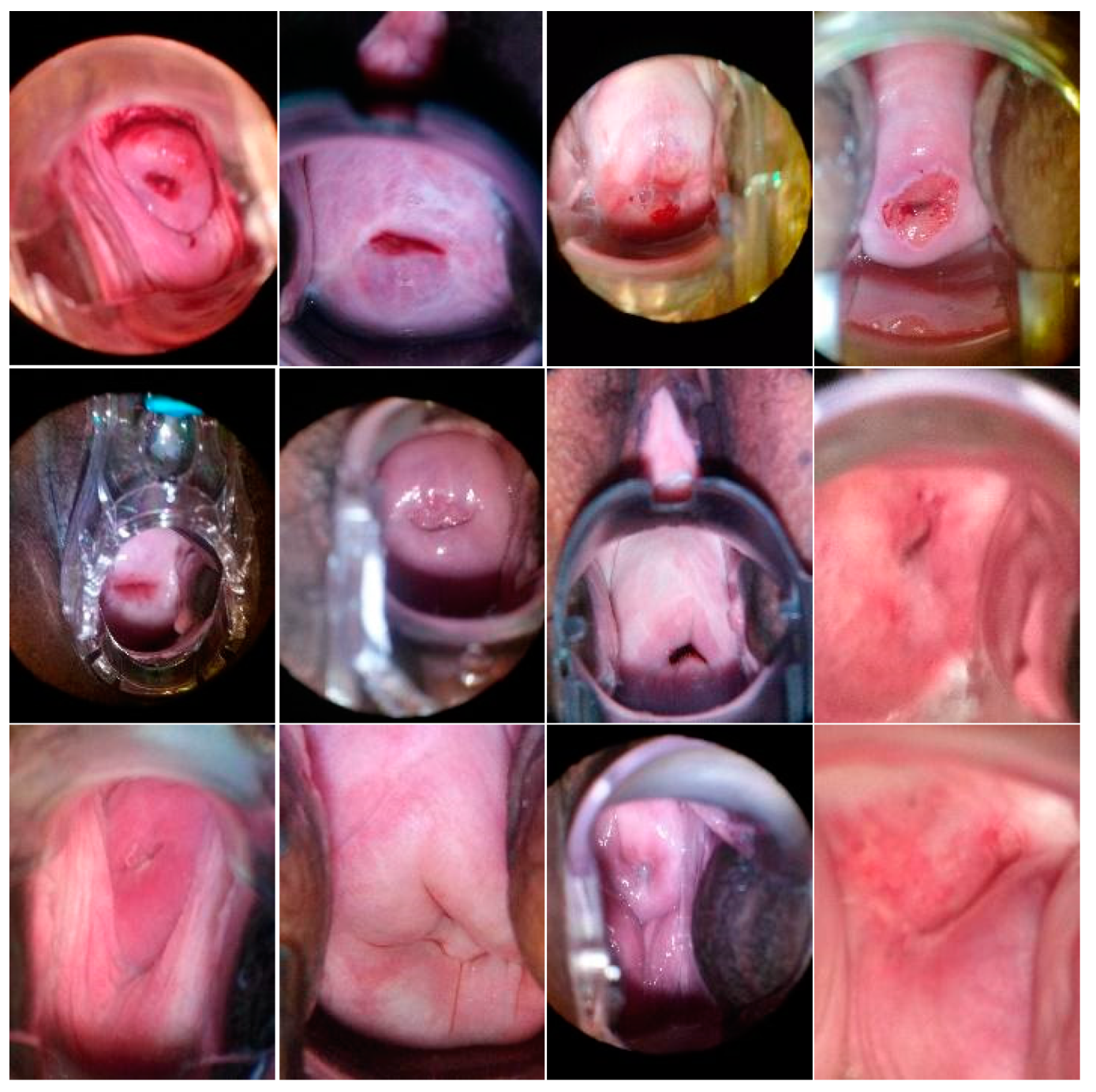
3. Data
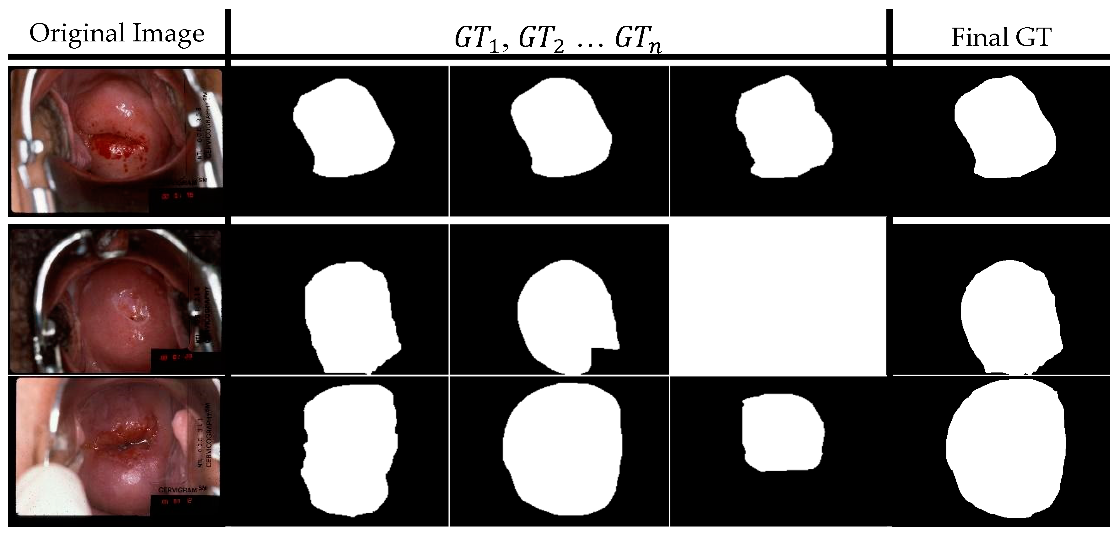
3.1. CVT Dataset
3.2. ALTS Dataset
3.3. Kaggle Dataset
4. Methods
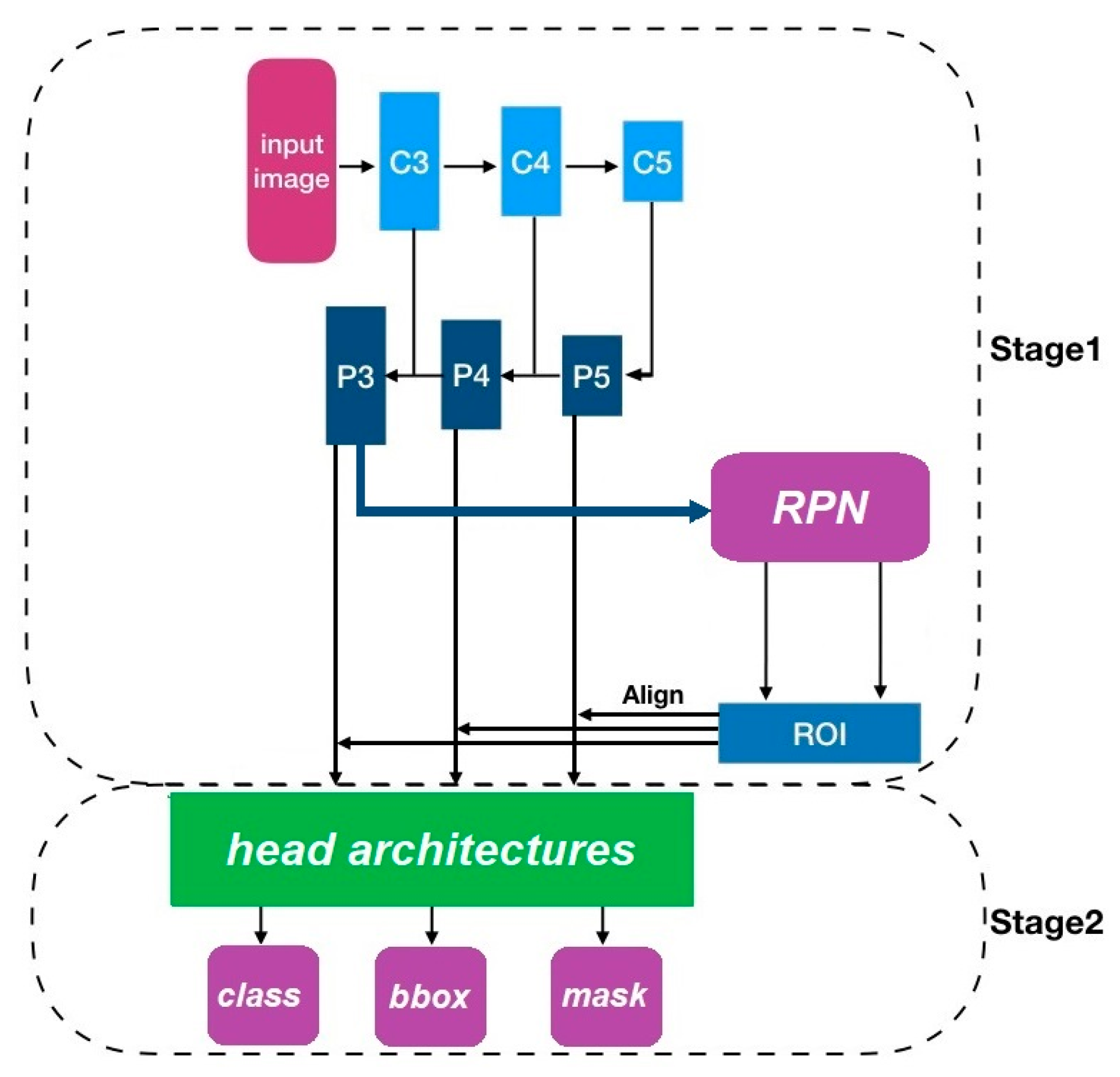
4.1. Mask R-CNN
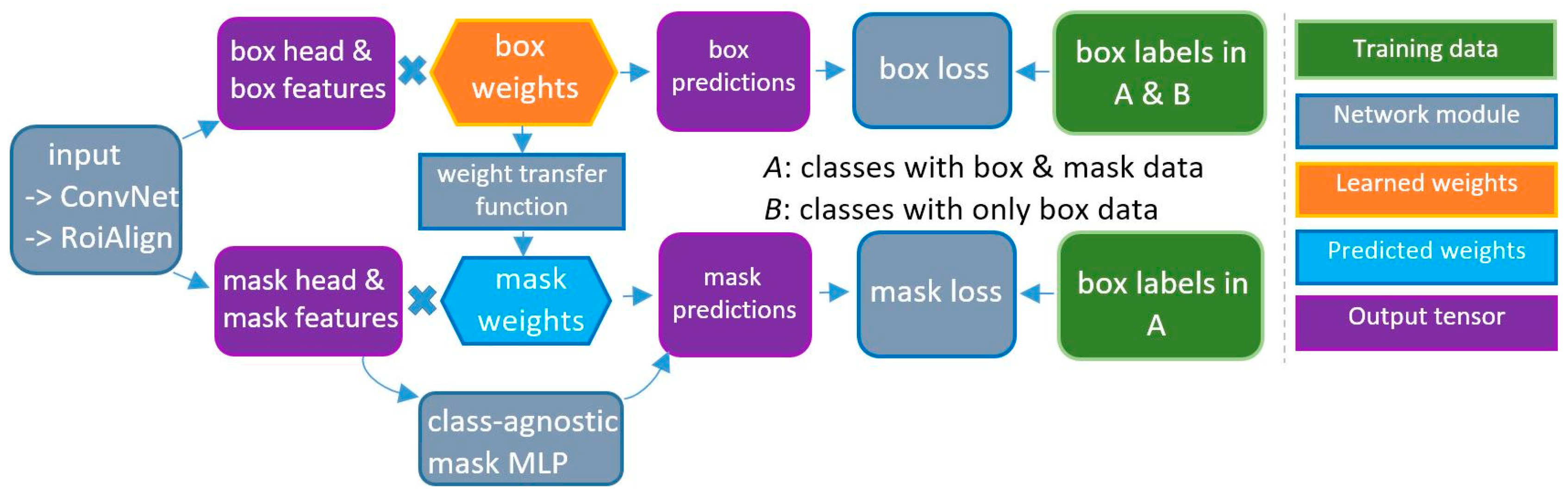
4.2. MaskX R-CNN
4.2.1. Stage-Wise Training
4.2.2. End-to-End Training
4.3. Implementation Details
5. Evaluation and Discussion
5.1. Single- and Cross-Dataset Training and Testing
5.2. Boosting with Bounding Box Information and MaskX R-CNN
5.3. Modified Weak Annotation
5.4. Multi-Datasets Training and Testing
5.5. Comparing Stage-Wise Training to End-to-End Training
5.6. Error Cases
6. Conclusions
Author Contributions
Funding
Acknowledgments
Conflicts of Interest
References
- World Health Organization. Human Papillomavirus (HPV) and Cervical Cancer World Health Organization. 24 January 2019. Available online: https://www.who.int/en/news-room/fact-sheets/detail/human-papillomavirus-(hpv)-and-cervical-cancer (accessed on 30 January 2019).
- Tao, L.; Amanguli, A.; Li, F.; Wang, Y.H.; Yang, L.; Mohemaiti, M.; Zhao, J.; Zou, X.G.; Saimaiti, A.; Abudu, M.; et al. Cervical Screening by Pap Test and Visual Inspection Enabling Same-Day Biopsy in Low-Resource. Obstet. Gynecol. 2018, 132, 1421–1429. [Google Scholar] [CrossRef] [PubMed]
- Jeronimo, J.; Massad, L.S.; Castle, P.E.; Wacholder, S.; Schiffman, M. National Institutes of Health (NIH)-American Society for Colposcopy and Cervical Pathology (ASCCP) Research Group. Interobserver agreement in the evaluation of digitized cervical images Obstetrics and gynecology. Obstet. Gynecol. 2007, 110, 833–840. [Google Scholar] [CrossRef] [PubMed]
- Hu, L.; Bell, D.; Antani, S.; Xue, Z.; Yu, K.; Horning, M.P.; Gachuhi, N.; Wilson, B.; Jaiswal, M.S.; Befano, B.; et al. An observational study of deep learning and automated evaluation of cervical images for cancer screening. J. Nat. Cancer Inst. 2019, 111, 923–932. [Google Scholar] [CrossRef] [PubMed]
- Jordan, J.; Singer, A.; Jones, H.; Shafi, M. The Cervix; Wiley: Hoboken, NJ, USA, 2009; pp. 23–29. [Google Scholar]
- Intel & MobileODT Cervical Cancer Screening Competition. 2017. Available online: https://www.kaggle.com/c/intel-mobileodt-cervical-cancer-screening (accessed on 8 December 2019).
- Guo, P.; Singh, S.; Xue, Z.; Long, R.; Antani, S. Deep Learning for Assessing Image Focus for Automated Cervical Cancer Screening. Presented at the IEEE International Conference on Biomedical and Health Informatics, Chicago, IL, USA, 19–22 May 2019. [Google Scholar]
- Zhu, Y.; Huang, X.; Wang, W.; Lopresti, D.; Long, R.; Antani, S.; Xue, Z.; Thoma, G. Balancing the Role of Priors in Multi-Observer Segmentation Evaluation. J. Signal Process. Syst. 2008, 1, 185–207. [Google Scholar] [CrossRef] [PubMed][Green Version]
- He, K.; Gkioxari, G.; Dollár, P.; Girshick, R. Mask R-CNN. In Proceedings of the IEEE International Conference on Computer Vision, Venice, Italy, 22–27 October 2017. [Google Scholar]
- Hu, R.; Dollár, P.; He, K.; Darrell, T. Girshick RLearning to Segment Every Thing. In Proceedings of the IEEE International Conference on Computer Vision, Venice, Italy, 22–27 October 2017. [Google Scholar]
- Bai, B.; Liu, P.Z.; Du, Y.Z.; Luo, Y.M. Automatic segmentation of cervical region in colposcopy images using K-means. Aus. Phys. Eng. Sci. Med. 2018, 41, 1077–1085. [Google Scholar] [CrossRef] [PubMed]
- Liu, J.; Li, L.; Wang, L. Acetowhite region segmentation in uterine cervix images using a registered ratio image. Comput. Biol. Med. 2018, 93, 47–55. [Google Scholar] [CrossRef] [PubMed]
- Kudva, V.; Prasad, K.; Guruvare, S. Detection of Specular Reflection and Segmentation of Cervix Region in Uterine Cervix Images for Cervical Cancer Screening. Innov. Res. Biomed. Eng. 2017, 38, 281–291. [Google Scholar] [CrossRef]
- Greenspan, H.; Gordon, S.; Zimmerman, G.; Lotenberg, S.; Jeronimo, J.; Antani, S.; Long, R. Automatic Detection of Anatomical Landmarks in Uterine Cervix Images. Trans. Med. Imaging 2008, 22, 286–296. [Google Scholar] [CrossRef] [PubMed]
- Xue, Z.; Long, L.R.; Antani, S.; Neve, L.; Zhu, Y.; Thoma, G.R. A unified set of analysis tools for uterine cervix image segmentation. Comput. Med. Imaging Graph. 2010, 34, 593–604. [Google Scholar] [CrossRef] [PubMed]
- Lotenberg, S.; Gordon, S.; Greenspan, H. Shape priors for segmentation of the cervix region within uterine cervix images. J. Digit. Imaging 2008, 22, 286–296. [Google Scholar] [CrossRef] [PubMed]
- Das, A.; Kar, A.; Bhattacharyya, D. Early Detection of Cervical Cancer Using Novel Segmentation Algorithms Invertis. J. Sci. Technol. 2014, 7, 91–95. [Google Scholar]
- Yu, Y.; Huang, J.; Zhang, S.; Restif, C.; Huang, X.; Metaxas, D. Group sparsity based classification for cervigram segmentation. In Proceedings of the IEEE International Symposium on Biomedical Imaging: From Nano to Macro, Chicago, IL, USA, 30 March–2 April 2011; pp. 1425–1429. [Google Scholar]
- Zhang, S.; Huang, J.; Metaxas, D.; Wang, W.; Huang, X. Discriminative sparse representations for cervigram image segmentation. In Proceedings of the IEEE International Symposium on Biomedical Imaging: From Nano to Macro, Rotterdam, The Netherlands, 14–17 April 2010; pp. 133–136. [Google Scholar]
- Zhang, S.; Huang, J.; Wang, W.; Huang, X.; Metaxas, D. Cervigram image segmentation based on reconstructive sparse representations. In Proceedings of the SPIE: Meical Imaging, San Diego, CA, USA, 12 March 2010. [Google Scholar] [CrossRef]
- Olaf, R.; Philipp, F.; Brox, T. U-Net: Convolutional Networks for Biomedical Image Segmentation. In Proceedings of the Computer Vision and Pattern Recognition, Boston, MA, USA, 8–10 June 2015. [Google Scholar]
- Zhang, X.; Zhao, S.G. Cervical image classification based on image segmentation preprocessing and a CapsNet network model. Int. J. Imaging Syst. Technol. 2019, 29, 19–28. [Google Scholar] [CrossRef]
- Fernandes, K.; Cardoso, J.S.; Fernandes, J. Cardoso. Automated Methods for the Decision Support of Cervical Cancer Screening Using Digital Colposcopies. IEEE Access 2018, 6, 33910–33927. [Google Scholar] [CrossRef]
- Fernandes, K.; Cardoso, J.S. Ordinal Image Segmentation using Deep Neural Networks. In Proceedings of the International Joint Conference on Neural Networks, Rio de Janeiro, Brazil, 8–13 July 2018. [Google Scholar]
- Fernandes, K.; Cruz, R.; Cardoso, J.S. Deep Image Segmentation by Quality Inference. In Proceedings of the International Joint Conference on Neural Networks, Rio de Janeiro, Brazil, 8–13 July 2018. [Google Scholar]
- Gorantla, R.; Singh, R.K.; Pandey, R.; Jain, M. Cervical Cancer Diagnosis Using CervixNet-A Deep Learning Approach. In Proceedings of the IEEE Conference (BIBE), Athens, Greece, 28–30 October 2019. [Google Scholar]
- Herrero, R.; Hildesheim, A.; Rodríguez, A.C.; Wacholder, S.; Bratti, C.; Solomon, D.; González, P.; Porras, C.; Jiménez, S.; Guillen, D.; et al. Rationale and design of a community-based double-blind randomized clinical trial of an HPV 16 and 18 vaccine in Guanacaste, Costa Rica. Vaccine 2008, 26, 4795–4808. [Google Scholar] [CrossRef] [PubMed]
- Herrero, R.; Wacholder, S.; Rodríguez, A.C.; Solomon, D.; González, P.; Kreimer, A.R.; Porras, C.; Schussler, J.; Jiménez, S.; Sherman, M.E.; et al. Prevention of persistent Human Papillomavirus Infection by an HPV16/18 vaccine: A community-based randomized clinical trial in Guanacaste, Costa Rica. Cancer Discov. 2011, 1, 408–419. [Google Scholar] [CrossRef] [PubMed]
- The Atypical Squamous Cells of Undetermined Significance/Low-Grade Squamous Intraepithelial Lesions Triage Study (ALTS) Group. Human Papillomavirus Testing for Triage of Women with Cytologic Evidence of Low-Grade Squamous Intraepithelial Lesions: Baseline Data from a Randomized Trial. J. Nat. Cancer Inst. 2000, 92, 397–402. [Google Scholar] [CrossRef] [PubMed]
- He, K.; Zhang, X.; Ren, S.; Sun, J. Deep Residual Learning for Image Recognition. In Proceedings of the IEEE International Conference on Computer Vision, Santiago Chile, 13–16 December 2015. [Google Scholar]
- Ren, S.; He, K.; Girshick, R.; Sun, J. Faster R-CNN: Towards Real-Time Object Detection with Region Proposal Networks. IEEE Trans. Pattern Anal. Mach. Intell. 2016, 6, 1137–1149. [Google Scholar] [CrossRef] [PubMed]
- Lin, T.Y.; Dollár, P.; Girshick, R.; He, K.; Hariharan, B.; Belongie, S. Feature Pyramid Networks for Object Detection. In Proceedings of the Computer Vision and Pattern Recognition, Honolulu, HI, USA, 21–26 July 2017. [Google Scholar]


| Dataset | Training Split | Testing Split |
|---|---|---|
| A | 2797 (from 1354 women) | 601 (from 320 women) |
| B | This dataset contains 939 images, which are used, either (1) all as training data; or (2) all as testing data. All the images have mask annotations and box annotations. | |
| C | 1448 | 502 |
| Training Dataset | BaseNet | Testing Results on A | |||
|---|---|---|---|---|---|
| Mask R-CNN | MaskX R-CNN | ||||
| Dice | IoU | Dice | IoU | ||
| A | ResNet50 | 0.9446 | 0.8970 | 0.9405 | 0.8902 |
| ResNet101 | 0.9438 | 0.8960 | 0.9418 | 0.8925 | |
| C | ResNet50 | 0.9107 | 0.8401 | 0.8664 | 0.7711 |
| ResNet101 | 0.9164 | 0.8497 | 0.8902 | 0.8075 | |
| Testing Results on C | |||||
| A | ResNet50 | 0.7385 | 0.6296 | 0.7798 | 0.6646 |
| ResNet101 | 0.7578 | 0.6456 | 0.7704 | 0.6547 | |
| C | ResNet50 | 0.9106 | 0.8572 | 0.8788 | 0.8058 |
| ResNet101 | 0.9197 | 0.8673 | 0.8867 | 0.8153 | |
| Ref. | Images | Measurements |
|---|---|---|
| [11] | 110 from 100 women | IoU: 0.79 |
| [12] | NA | IoU: 0.76 |
| [13] | 151 | Dice: 0.90 |
| [14] | 278 (subset of Dataset B) | Dice: 0.75 |
| [16] | 378 (subset of Dataset B) | Dice: 0.81 |
| [17] | 250 from 4 women | AUC: 0.90 |
| [18,19,20] | 100 | sensitivity: 0.71 specificity: 0.82 |
| [22] | Dataset A | IoU: 0.74 |
| [23,24,25] | 1480 (Dataset C) | Dice: 0.67 |
| [26] | Dataset A | (Dice, IoU): (0.8711, 0.765) |
| Training Dataset | BaseNet | Testing Results on B | |||
|---|---|---|---|---|---|
| Mask R-CNN | MaskX R-CNN | ||||
| Dice | IoU | Dice | IoU | ||
| A | ResNet50 | 0.8443 | 0.7522 | 0.8345 | 0.7377 |
| ResNet101 | 0.8481 | 0.7569 | 0.8359 | 0.7395 | |
| C | ResNet50 | 0.8863 | 0.8166 | 0.8700 | 0.7904 |
| ResNet101 | 0.8873 | 0.8186 | 0.8747 | 0.7976 | |
| Training Dataset | BaseNet | Testing Results on A | Testing Results on C | ||
|---|---|---|---|---|---|
| Dice | IoU | Dice | IoU | ||
| A + | ResNet50 | 0.9418 | 0.8922 | 0.8993 | 0.8220 |
| ResNet101 | 0.9410 | 0.8910 | 0.8910 | 0.8093 | |
| Training Dataset | Dynamic Modifier | Testing Results on A | Testing Results on C | ||
|---|---|---|---|---|---|
| Dice | IoU | Dice | IoU | ||
| A + | 10 pixels | 0.9376 | 0.8850 | 0.8635 | 0.7670 |
| 20 pixels | 0.9369 | 0.8829 | 0.8280 | 0.7164 | |
| Rand (0, 35) pixels | 0.9387 | 0.8863 | 0.8413 | 0.7350 | |
| Training Dataset | Testing Dataset | BaseNet | Mask R-CNN | MaskX R-CNN | ||
|---|---|---|---|---|---|---|
| Dice | IoU | Dice | IoU | |||
| A + C | A | ResNet50 | 0.9446 | 0.8971 | 0.9138 | 0.8458 |
| ResNet101 | 0.9469 | 0.9009 | 0.9231 | 0.8622 | ||
| C | ResNet50 | 0.9161 | 0.8630 | 0.8866 | 0.8073 | |
| ResNet101 | 0.9200 | 0.8694 | 0.8758 | 0.7908 | ||
| A + B | A | ResNet50 | 0.9442 | 0.8966 | 0.9437 | 0.8956 |
| ResNet101 | 0.9442 | 0.8964 | 0.9421 | 0.8932 | ||
| C | ResNet50 | 0.8176 | 0.7230 | 0.8158 | 0.7159 | |
| ResNet101 | 0.8219 | 0.7216 | 0.8066 | 0.7017 | ||
| A + B + C | A | ResNet50 | 0.9454 | 0.8985 | 0.9376 | 0.8852 |
| ResNet101 | 0.9462 | 0.8999 | 0.9325 | 0.8713 | ||
| C | ResNet50 | 0.9159 | 0.8623 | 0.8985 | 0.8228 | |
| ResNet101 | 0.9213 | 0.8700 | 0.8904 | 0.8010 | ||
| A + B + C(box) | A | ResNet50 | N/A | N/A | 0.9387 | 0.8870 |
| ResNet101 | N/A | N/A | 0.9376 | 0.8857 | ||
| C | ResNet50 | N/A | N/A | 0.8915 | 0.8102 | |
| ResNet101 | N/A | N/A | 0.8866 | 0.8021 | ||
| A(box) + B + C(box) | A | ResNet50 | N/A | N/A | 0.9244 | 0.8623 |
| ResNet101 | N/A | N/A | 0.9050 | 0.8311 | ||
| C | ResNet50 | N/A | N/A | 0.8841 | 0.7966 | |
| ResNet101 | N/A | N/A | 0.8819 | 0.7945 | ||
| A(box) + B + C | A | ResNet50 | N/A | N/A | 0.9318 | 0.8751 |
| ResNet101 | N/A | N/A | 0.9353 | 0.8809 | ||
| C | ResNet50 | N/A | N/A | 0.8962 | 0.8190 | |
| ResNet101 | N/A | N/A | 0.8869 | 0.8038 | ||
| A(box) + B(box) + C | A | ResNet50 | N/A | N/A | 0.9294 | 0.8710 |
| ResNet101 | N/A | N/A | 0.9308 | 0.8732 | ||
| C | ResNet50 | N/A | N/A | 0.8928 | 0.8139 | |
| ResNet101 | N/A | N/A | 0.8906 | 0.8096 | ||
| Training Dataset | Training Strategy | MaskX R-CNN | |||
|---|---|---|---|---|---|
| Testing Results on A | Testing Results on C | ||||
| Dice | IoU | Dice | IoU | ||
| A + C | Stage-wise | 0.9138 | 0.8458 | 0.8866 | 0.8073 |
| End-to-end | 0.9452 | 0.8980 | 0.9081 | 0.8368 | |
© 2020 by the authors. Licensee MDPI, Basel, Switzerland. This article is an open access article distributed under the terms and conditions of the Creative Commons Attribution (CC BY) license (http://creativecommons.org/licenses/by/4.0/).
Share and Cite
Guo, P.; Xue, Z.; Long, L.R.; Antani, S. Cross-Dataset Evaluation of Deep Learning Networks for Uterine Cervix Segmentation. Diagnostics 2020, 10, 44. https://doi.org/10.3390/diagnostics10010044
Guo P, Xue Z, Long LR, Antani S. Cross-Dataset Evaluation of Deep Learning Networks for Uterine Cervix Segmentation. Diagnostics. 2020; 10(1):44. https://doi.org/10.3390/diagnostics10010044
Chicago/Turabian StyleGuo, Peng, Zhiyun Xue, L. Rodney Long, and Sameer Antani. 2020. "Cross-Dataset Evaluation of Deep Learning Networks for Uterine Cervix Segmentation" Diagnostics 10, no. 1: 44. https://doi.org/10.3390/diagnostics10010044
APA StyleGuo, P., Xue, Z., Long, L. R., & Antani, S. (2020). Cross-Dataset Evaluation of Deep Learning Networks for Uterine Cervix Segmentation. Diagnostics, 10(1), 44. https://doi.org/10.3390/diagnostics10010044