
PathoLive—Real-Time Pathogen Identification from Metagenomic Illumina Datasets

 , ,
, ,  , and
, and
Abstract
1. Introduction
2. Methods
2.1. Implementation
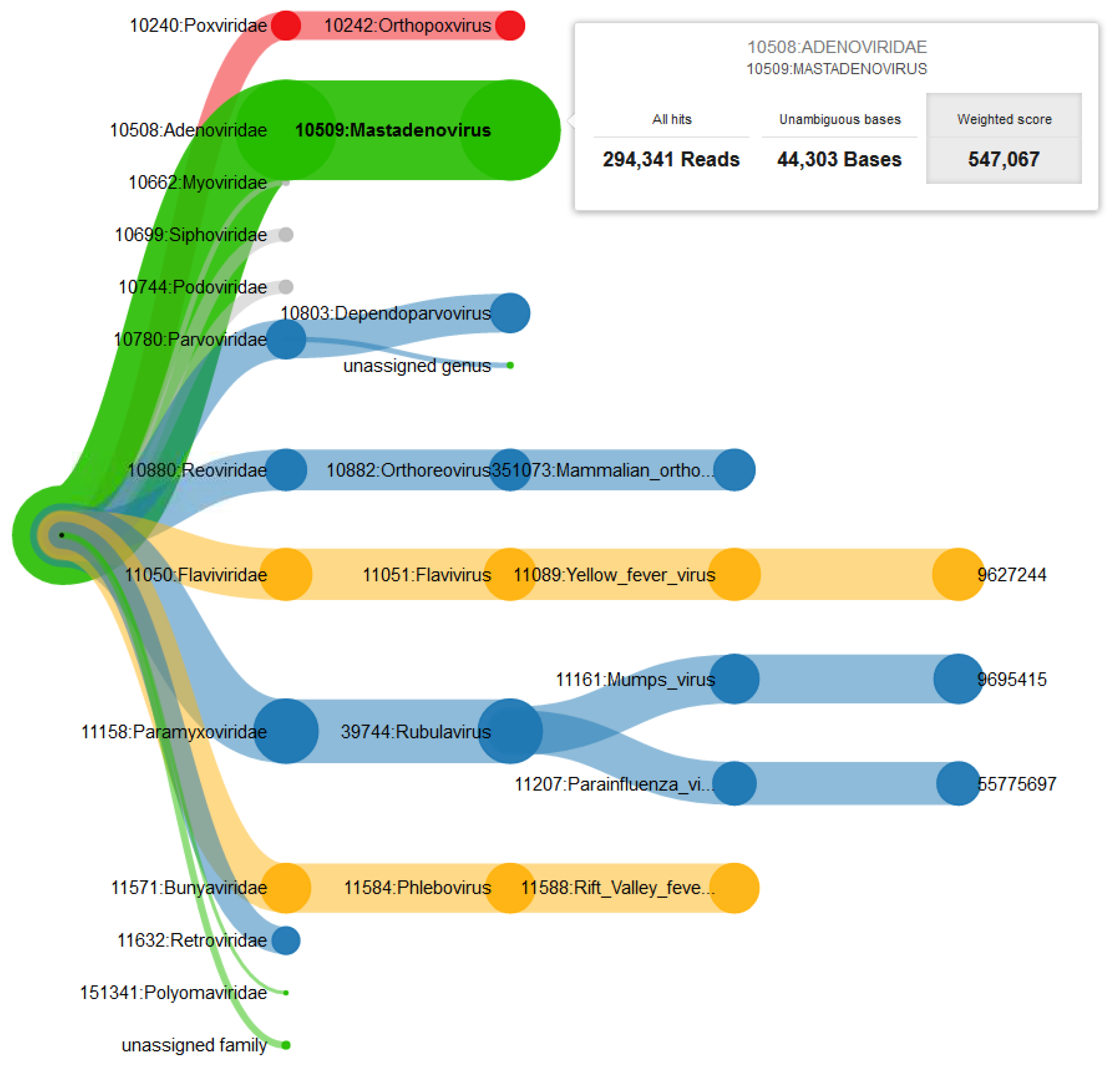
- (a)
- Total hits , representing the total number of hits to all underlying sequences in this branch: , representing the total abundance of a clade.
- (b)
- Unambiguous bases , representing the total number of bases covered in the foreground data but not in any background dataset:
- (c)
- Weighted score , being the ratio of unambiguous bases for the foreground data to the number of bases covered by the background database and logarithmically weighted by the total number of alignments:
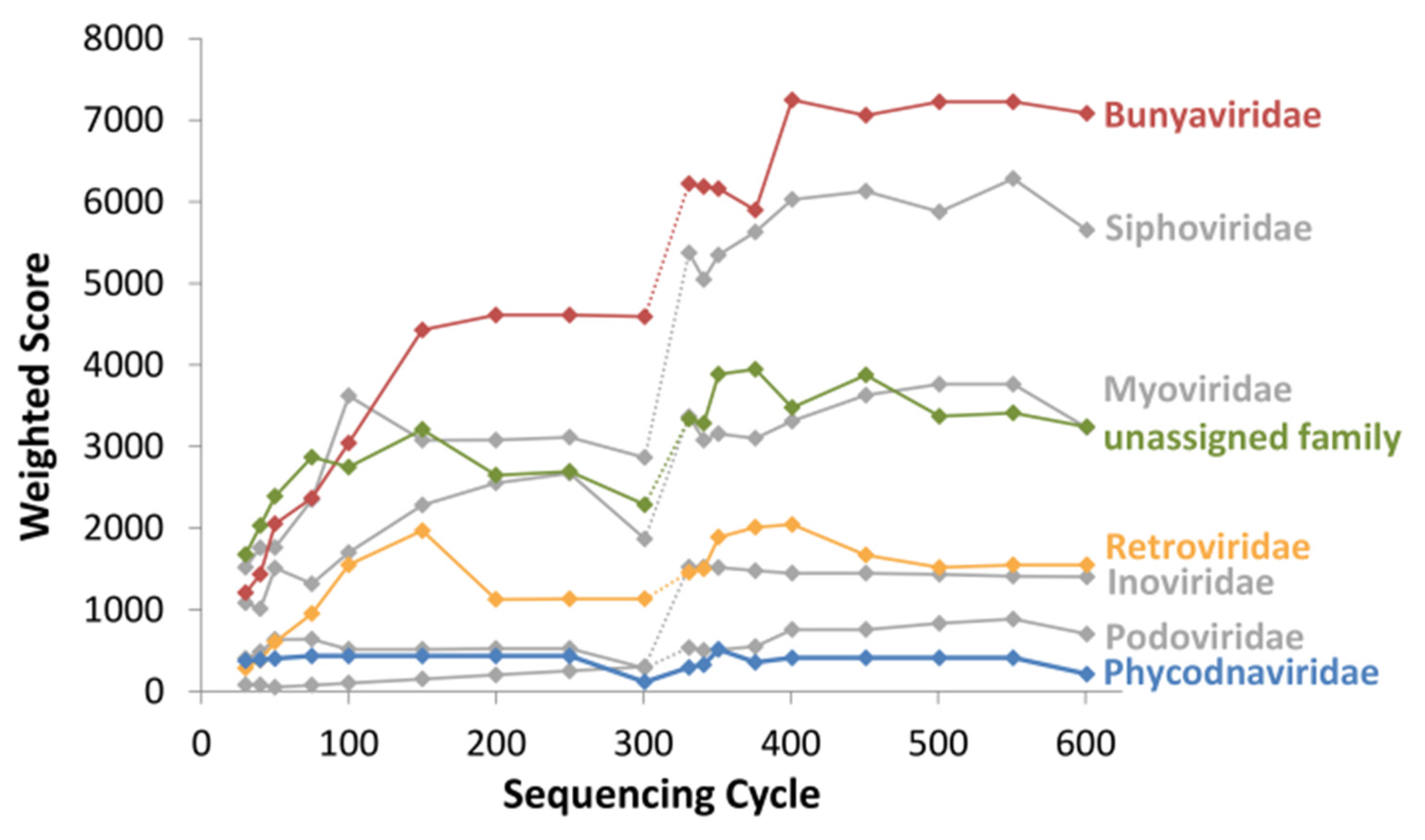
2.2. Validation
2.3. Sample Preparation
3. Results
3.1. Pathogen Detection in a Spiked Viral Mixture
3.2. Identification of Crimean-Congo Hemorrhagic Fever Virus in a Real Sample from Sudan
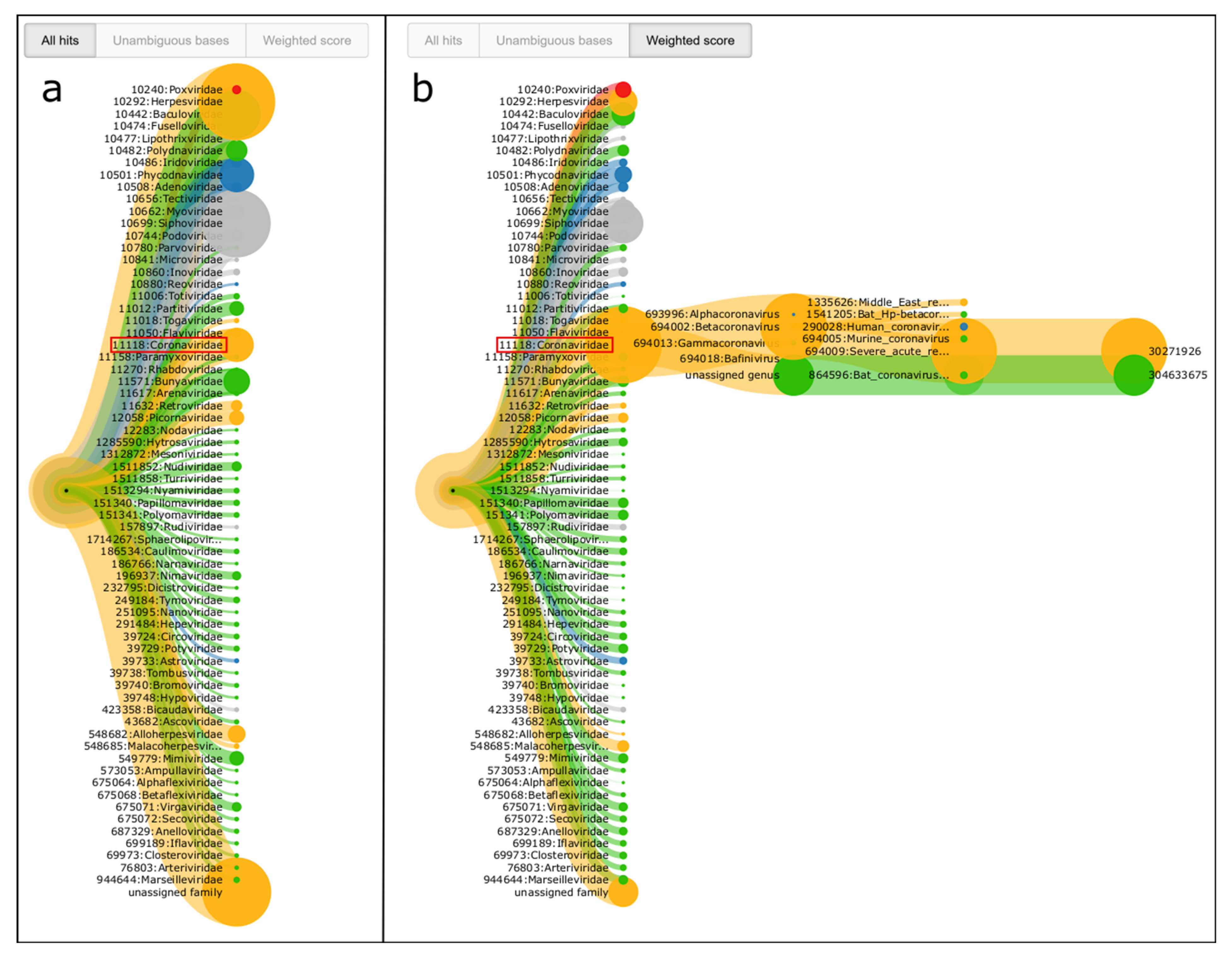
3.3. Detection of a Coronavirus in a Real Sample from the 2019 SARS-CoV-2 Outbreak in Wuhan
4. Discussion
Supplementary Materials
Author Contributions
Funding
Data Availability Statement
Acknowledgments
Conflicts of Interest
References
- Bzhalava, D.; Johansson, H.; Ekstrom, J.; Faust, H.; Moller, B.; Eklund, C.; Nordin, P.; Stenquist, B.; Paoli, J.; Persson, B.; et al. Unbiased approach for virus detection in skin lesions. PLoS ONE 2013, 8, e65953. [Google Scholar] [CrossRef] [PubMed]
- Greninger, A.L.; Zerr, D.M.; Qin, X.; Adler, A.L.; Sampoleo, R.; Kuypers, J.M.; Englund, J.A.; Jerome, K.R. Rapid Metagenomic Next-Generation Sequencing during an Investigation of Hospital-Acquired Human Parainfluenza Virus 3 Infections. J. Clin. Microbiol. 2017, 55, 177–182. [Google Scholar] [CrossRef] [PubMed]
- Breitwieser, F.P.; Pardo, C.A.; Salzberg, S.L. Re-analysis of metagenomic sequences from acute flaccid myelitis patients reveals alternatives to enterovirus D68 infection. F1000Research 2015, 4, 180. [Google Scholar] [CrossRef] [PubMed]
- Salzberg, S.L.; Breitwieser, F.P.; Kumar, A.; Hao, H.; Burger, P.; Rodriguez, F.J.; Lim, M.; Quinones-Hinojosa, A.; Gallia, G.L.; Tornheim, J.A.; et al. Next-generation sequencing in neuropathologic diagnosis of infections of the nervous system. Neurol. Neuroimmunol. Neuroinflamm. 2016, 3, e251. [Google Scholar] [CrossRef] [PubMed]
- Cao, M.D.; Ganesamoorthy, D.; Elliott, A.G.; Zhang, H.; Cooper, M.A.; Coin, L.J. Streaming algorithms for identification of pathogens and antibiotic resistance potential from real-time MinION(TM) sequencing. Gigascience 2016, 5, 32. [Google Scholar] [CrossRef]
- Roux, S.; Tournayre, J.; Mahul, A.; Debroas, D.; Enault, F. Metavir 2: New tools for viral metagenome comparison and assembled virome analysis. BMC Bioinform. 2014, 15, 76. [Google Scholar] [CrossRef]
- Kostic, A.D.; Ojesina, A.I.; Pedamallu, C.S.; Jung, J.; Verhaak, R.G.; Getz, G.; Meyerson, M. PathSeq: Software to identify or discover microbes by deep sequencing of human tissue. Nat. Biotechnol. 2011, 29, 393–396. [Google Scholar] [CrossRef]
- Skewes-Cox, P.; Sharpton, T.J.; Pollard, K.S.; DeRisi, J.L. Profile hidden Markov models for the detection of viruses within metagenomic sequence data. PLoS ONE 2014, 9, e105067. [Google Scholar] [CrossRef]
- Wommack, K.E.; Bhavsar, J.; Polson, S.W.; Chen, J.; Dumas, M.; Srinivasiah, S.; Furman, M.; Jamindar, S.; Nasko, D.J. VIROME: A standard operating procedure for analysis of viral metagenome sequences. Stand. Genom. Sci. 2012, 6, 427–439. [Google Scholar] [CrossRef]
- Dutilh, B.E.; Schmieder, R.; Nulton, J.; Felts, B.; Salamon, P.; Edwards, R.A.; Mokili, J.L. Reference-independent comparative metagenomics using cross-assembly: crAss. Bioinformatics 2012, 28, 3225–3231. [Google Scholar] [CrossRef]
- Norling, M.; Karlsson-Lindsjo, O.E.; Gourle, H.; Bongcam-Rudloff, E.; Hayer, J. MetLab: An In Silico Experimental Design, Simulation and Analysis Tool for Viral Metagenomics Studies. PLoS ONE 2016, 11, e0160334. [Google Scholar] [CrossRef] [PubMed]
- Huson, D.H.; Beier, S.; Flade, I.; Gorska, A.; El-Hadidi, M.; Mitra, S.; Ruscheweyh, H.J.; Tappu, R. MEGAN Community Edition—Interactive Exploration and Analysis of Large-Scale Microbiome Sequencing Data. PLoS Comput. Biol. 2016, 12, e1004957. [Google Scholar] [CrossRef] [PubMed]
- Zhao, G.; Wu, G.; Lim, E.S.; Droit, L.; Krishnamurthy, S.; Barouch, D.H.; Virgin, H.W.; Wang, D. VirusSeeker, a computational pipeline for virus discovery and virome composition analysis. Virology 2017, 503, 21–30. [Google Scholar] [CrossRef]
- Tausch, S.H.; Renard, B.Y.; Nitsche, A.; Dabrowski, P.W. RAMBO-K: Rapid and Sensitive Removal of Background Sequences from Next Generation Sequencing Data. PLoS ONE 2015, 10, e0137896. [Google Scholar] [CrossRef]
- Piro, V.C.; Matschkowski, M.; Renard, B.Y. MetaMeta: Integrating metagenome analysis tools to improve taxonomic profiling. Microbiome 2017, 5, 101. [Google Scholar] [CrossRef] [PubMed]
- Bray, N.L.; Pimentel, H.; Melsted, P.; Pachter, L. Near-optimal probabilistic RNA-seq quantification. Nat. Biotechnol. 2016, 34, 525–527. [Google Scholar] [CrossRef]
- Menzel, P.; Ng, K.L.; Krogh, A. Fast and sensitive taxonomic classification for metagenomics with Kaiju. Nat. Commun. 2016, 7, 11257. [Google Scholar] [CrossRef]
- Zheng, Y.; Gao, S.; Padmanabhan, C.; Li, R.; Galvez, M.; Gutierrez, D.; Fuentes, S.; Ling, K.S.; Kreuze, J.; Fei, Z. VirusDetect: An automated pipeline for efficient virus discovery using deep sequencing of small RNAs. Virology 2017, 500, 130–138. [Google Scholar] [CrossRef]
- Dadi, T.H.; Renard, B.Y.; Wieler, L.H.; Semmler, T.; Reinert, K. SLIMM: Species level identification of microorganisms from metagenomes. PeerJ 2017, 5, e3138. [Google Scholar] [CrossRef] [PubMed]
- Lee, A.Y.; Lee, C.S.; Van Gelder, R.N. Scalable metagenomics alignment research tool (SMART): A scalable, rapid, and complete search heuristic for the classification of metagenomic sequences from complex sequence populations. BMC Bioinform. 2016, 17, 292. [Google Scholar] [CrossRef]
- Piro, V.C.; Lindner, M.S.; Renard, B.Y. DUDes: A top-down taxonomic profiler for metagenomics. Bioinformatics 2016, 32, 2272–2280. [Google Scholar] [CrossRef]
- Wood, D.E.; Salzberg, S.L. Kraken: Ultrafast metagenomic sequence classification using exact alignments. Genome Biol 2014, 15, R46. [Google Scholar] [CrossRef] [PubMed]
- Truong, D.T.; Franzosa, E.A.; Tickle, T.L.; Scholz, M.; Weingart, G.; Pasolli, E.; Tett, A.; Huttenhower, C.; Segata, N. MetaPhlAn2 for enhanced metagenomic taxonomic profiling. Nat. Methods 2015, 12, 902–903. [Google Scholar] [CrossRef] [PubMed]
- Scheuch, M.; Hoper, D.; Beer, M. RIEMS: A software pipeline for sensitive and comprehensive taxonomic classification of reads from metagenomics datasets. BMC Bioinform. 2015, 16, 69. [Google Scholar] [CrossRef]
- Hong, C.; Manimaran, S.; Shen, Y.; Perez-Rogers, J.F.; Byrd, A.L.; Castro-Nallar, E.; Crandall, K.A.; Johnson, W.E. PathoScope 2.0: A complete computational framework for strain identification in environmental or clinical sequencing samples. Microbiome 2014, 2, 33. [Google Scholar] [CrossRef]
- Byrd, A.L.; Perez-Rogers, J.F.; Manimaran, S.; Castro-Nallar, E.; Toma, I.; McCaffrey, T.; Siegel, M.; Benson, G.; Crandall, K.A.; Johnson, W.E. Clinical PathoScope: Rapid alignment and filtration for accurate pathogen identification in clinical samples using unassembled sequencing data. BMC Bioinform. 2014, 15, 262. [Google Scholar] [CrossRef] [PubMed]
- Francis, O.E.; Bendall, M.; Manimaran, S.; Hong, C.; Clement, N.L.; Castro-Nallar, E.; Snell, Q.; Schaalje, G.B.; Clement, M.J.; Crandall, K.A.; et al. Pathoscope: Species identification and strain attribution with unassembled sequencing data. Genome Res. 2013, 23, 1721–1729. [Google Scholar] [CrossRef] [PubMed]
- Flygare, S.; Simmon, K.; Miller, C.; Qiao, Y.; Kennedy, B.; Di Sera, T.; Graf, E.H.; Tardif, K.D.; Kapusta, A.; Rynearson, S.; et al. Taxonomer: An interactive metagenomics analysis portal for universal pathogen detection and host mRNA expression profiling. Genome Biol. 2016, 17, 111. [Google Scholar] [CrossRef]
- Lindner, M.S.; Renard, B.Y. Metagenomic abundance estimation and diagnostic testing on species level. Nucleic Acids Res. 2013, 41, e10. [Google Scholar] [CrossRef]
- Naccache, S.N.; Federman, S.; Veeraraghavan, N.; Zaharia, M.; Lee, D.; Samayoa, E.; Bouquet, J.; Greninger, A.L.; Luk, K.C.; Enge, B.; et al. A cloud-compatible bioinformatics pipeline for ultrarapid pathogen identification from next-generation sequencing of clinical samples. Genome Res. 2014, 24, 1180–1192. [Google Scholar] [CrossRef] [PubMed]
- Piro, V.C.; Dadi, T.H.; Seiler, E.; Reinert, K.; Renard, B.Y. ganon: Precise metagenomics classification against large and up-to-date sets of reference sequences. bioRxiv 2019, 406017. [Google Scholar] [CrossRef] [PubMed]
- Wood, D.E.; Lu, J.; Langmead, B. Improved metagenomic analysis with Kraken 2. Genome Biol. 2019, 20, 257. [Google Scholar] [CrossRef]
- Breitwieser, F.P.; Lu, J.; Salzberg, S.L. A review of methods and databases for metagenomic classification and assembly. Brief Bioinform 2017, 20, 1125–1136. [Google Scholar] [CrossRef] [PubMed]
- Dutilh, B.E.; Reyes, A.; Hall, R.J.; Whiteson, K.L. Editorial: Virus Discovery by Metagenomics: The (Im)possibilities. Front. Microbiol. 2017, 8, 1710. [Google Scholar] [CrossRef] [PubMed]
- Frey, K.G.; Herrera-Galeano, J.E.; Redden, C.L.; Luu, T.V.; Servetas, S.L.; Mateczun, A.J.; Mokashi, V.P.; Bishop-Lilly, K.A. Comparison of three next-generation sequencing platforms for metagenomic sequencing and identification of pathogens in blood. BMC Genom. 2014, 15, 96. [Google Scholar] [CrossRef]
- Lecuit, M.; Eloit, M. The diagnosis of infectious diseases by whole genome next generation sequencing: A new era is opening. Front. Cell. Infect. Microbiol. 2014, 4, 25. [Google Scholar] [CrossRef]
- Lecuit, M.; Eloit, M. The potential of whole genome NGS for infectious disease diagnosis. Expert. Rev. Mol. Diagn. 2015, 15, 1517–1519. [Google Scholar] [CrossRef]
- Mokili, J.L.; Rohwer, F.; Dutilh, B.E. Metagenomics and future perspectives in virus discovery. Curr. Opin. Virol. 2012, 2, 63–77. [Google Scholar] [CrossRef]
- Roux, S.; Emerson, J.B.; Eloe-Fadrosh, E.A.; Sullivan, M.B. Benchmarking viromics: An in silico evaluation of metagenome-enabled estimates of viral community composition and diversity. PeerJ 2017, 5, e3817. [Google Scholar] [CrossRef]
- Snyder, L.A.; Loman, N.; Pallen, M.J.; Penn, C.W. Next-generation sequencing--the promise and perils of charting the great microbial unknown. Microb. Ecol. 2009, 57, 1–3. [Google Scholar] [CrossRef]
- Breitwieser, F.P.; Pertea, M.; Zimin, A.V.; Salzberg, S.L. Human contamination in bacterial genomes has created thousands of spurious proteins. Genome Res. 2019, 29, 954–960. [Google Scholar] [CrossRef] [PubMed]
- Quick, J.; Ashton, P.; Calus, S.; Chatt, C.; Gossain, S.; Hawker, J.; Nair, S.; Neal, K.; Nye, K.; Peters, T.; et al. Rapid draft sequencing and real-time nanopore sequencing in a hospital outbreak of Salmonella. Genome Biol. 2015, 16, 114. [Google Scholar] [CrossRef] [PubMed]
- Stranneheim, H.; Engvall, M.; Naess, K.; Lesko, N.; Larsson, P.; Dahlberg, M.; Andeer, R.; Wredenberg, A.; Freyer, C.; Barbaro, M.; et al. Rapid pulsed whole genome sequencing for comprehensive acute diagnostics of inborn errors of metabolism. BMC Genom. 2014, 15, 1090. [Google Scholar] [CrossRef] [PubMed]
- Miller, N.A.; Farrow, E.G.; Gibson, M.; Willig, L.K.; Twist, G.; Yoo, B.; Marrs, T.; Corder, S.; Krivohlavek, L.; Walter, A.; et al. A 26-hour system of highly sensitive whole genome sequencing for emergency management of genetic diseases. Genome Med. 2015, 7, 100. [Google Scholar] [CrossRef] [PubMed]
- Tausch, S.H.; Strauch, B.; Andrusch, A.; Loka, T.P.; Lindner, M.S.; Nitsche, A.; Renard, B.Y. LiveKraken––Real-time metagenomic classification of illumina data. Bioinformatics 2018, 34, 3750–3752. [Google Scholar] [CrossRef]
- Greninger, A.L.; Naccache, S.N.; Federman, S.; Yu, G.; Mbala, P.; Bres, V.; Stryke, D.; Bouquet, J.; Somasekar, S.; Linnen, J.M.; et al. Rapid metagenomic identification of viral pathogens in clinical samples by real-time nanopore sequencing analysis. Genome Med. 2015, 7, 99. [Google Scholar] [CrossRef]
- Loose, M.; Malla, S.; Stout, M. Real-time selective sequencing using nanopore technology. Nat. Methods 2016, 13, 751–754. [Google Scholar] [CrossRef]
- Stewart, R.D.; Watson, M. poRe GUIs for parallel and real-time processing of MinION sequence data. Bioinformatics 2017, 33, 2207–2208. [Google Scholar] [CrossRef]
- Loka, T.P.; Tausch, S.H.; Renard, B.Y. Reliable variant calling during runtime of Illumina sequencing. Sci. Rep. 2019, 9, 16502. [Google Scholar] [CrossRef]
- Brister, J.R.; Ako-Adjei, D.; Bao, Y.; Blinkova, O. NCBI viral genomes resource. Nucleic Acids Res. 2015, 43, D571–D577. [Google Scholar] [CrossRef]
- The 1000 Genomes Project Consortium. A global reference for human genetic variation. Nature 2015, 526, 68–74. [Google Scholar] [CrossRef] [PubMed]
- Bolger, A.M.; Lohse, M.; Usadel, B. Trimmomatic: A flexible trimmer for Illumina sequence data. Bioinformatics 2014, 30, 2114–2120. [Google Scholar] [CrossRef] [PubMed]
- Langmead, B.; Salzberg, S.L. Fast gapped-read alignment with Bowtie 2. Nat Methods 2012, 9, 357–359. [Google Scholar] [CrossRef] [PubMed]
- Lindner, M.S.; Renard, B.Y. Metagenomic profiling of known and unknown microbes with microbeGPS. PLoS ONE 2015, 10, e0117711. [Google Scholar] [CrossRef]
- Bostock, M.; Ogievetsky, V.; Heer, J. D(3): Data-Driven Documents. IEEE Trans. Vis. Comput. Graph. 2011, 17, 2301–2309. [Google Scholar] [CrossRef]
- Biosafety and Biotechnology Unit. Belgian Classifications for Micro-Organisms Based on Their Biological Risks—Definitions. 20087. Available online: https://my.absa.org/Riskgroups (accessed on 23 August 2022).
- Lu, J.; Breitwieser, F.P.; Thielen, P.; Salzberg, S.L. Bracken: Estimating species abundance in metagenomics data. PeerJ Computer Science 2017, 3, e104. [Google Scholar] [CrossRef]
- O’Leary, N.A.; Wright, M.W.; Brister, J.R.; Ciufo, S.; Haddad, D.; McVeigh, R.; Rajput, B.; Robbertse, B.; Smith-White, B.; Ako-Adjei, D.; et al. Reference sequence (RefSeq) database at NCBI: Current status, taxonomic expansion, and functional annotation. Nucleic Acids Res 2016, 44, D733–D745. [Google Scholar] [CrossRef]
- Andrusch, A.; Dabrowski, P.W.; Klenner, J.; Tausch, S.H.; Kohl, C.; Osman, A.A.; Renard, B.Y.; Nitsche, A. PAIPline: Pathogen identification in metagenomic and clinical next generation sequencing samples. Bioinformatics 2018, 34, i715–i721. [Google Scholar] [CrossRef]
- Kohl, C.; Eldegail, M.; Mahmoud, I.; Schrick, L.; Radonic, A.; Emmerich, P.; Rieger, T.; Gunther, S.; Nitsche, A.; Osman, A.A. Crimean congo hemorrhagic fever, 2013 and 2014 Sudan. Int. J. Infect. Dis. 2016, 53, 9. [Google Scholar] [CrossRef][Green Version]
- Wu, F.; Zhao, S.; Yu, B.; Chen, Y.-M.; Wang, W.; Song, Z.-G.; Hu, Y.; Tao, Z.-W.; Tian, J.-H.; Pei, Y.-Y.; et al. A new coronavirus associated with human respiratory disease in China. Nature 2020, 579, 265–269. [Google Scholar] [CrossRef]
- Kohl, C.; Brinkmann, A.; Dabrowski, P.W.; Radonic, A.; Nitsche, A.; Kurth, A. Protocol for metagenomic virus detection in clinical specimens. Emerg. Infect. Dis. 2015, 21, 48–57. [Google Scholar] [CrossRef] [PubMed]
- Edwards, H.S.; Krishnakumar, R.; Sinha, A.; Bird, S.W.; Patel, K.D.; Bartsch, M.S. Real-Time Selective Sequencing with RUBRIC: Read Until with Basecall and Reference-Informed Criteria. Sci. Rep. 2019, 9, 11475. [Google Scholar] [CrossRef] [PubMed]


| Total Hits | Weighted Score | ||||
|---|---|---|---|---|---|
| Family | Hits | Family | Score | ||
| 1 | Herpesviridae | 21,811 | 1 | Coronaviridae | 46,274 |
| 2 | unassigned family | 17,345 | 2 | Siphoviridae | 11,559 |
| 3 | Siphoviridae | 16,838 | 3 | unassigned family | 6148 |
| 4 | Baculoviridae | 7996 | 4 | Herpesviridae | 5342 |
| 5 | Phycodnaviridae | 4018 | 5 | Myoviridae | 3775 |
| 6 | Coronaviridae | 3827 | 6 | Baculoviridae | 3423 |
| … | … | ||||
Publisher’s Note: MDPI stays neutral with regard to jurisdictional claims in published maps and institutional affiliations. |
© 2022 by the authors. Licensee MDPI, Basel, Switzerland. This article is an open access article distributed under the terms and conditions of the Creative Commons Attribution (CC BY) license (https://creativecommons.org/licenses/by/4.0/).
Share and Cite
Tausch, S.H.; Loka, T.P.; Schulze, J.M.; Andrusch, A.; Klenner, J.; Dabrowski, P.W.; Lindner, M.S.; Nitsche, A.; Renard, B.Y. PathoLive—Real-Time Pathogen Identification from Metagenomic Illumina Datasets. Life 2022, 12, 1345. https://doi.org/10.3390/life12091345
Tausch SH, Loka TP, Schulze JM, Andrusch A, Klenner J, Dabrowski PW, Lindner MS, Nitsche A, Renard BY. PathoLive—Real-Time Pathogen Identification from Metagenomic Illumina Datasets. Life. 2022; 12(9):1345. https://doi.org/10.3390/life12091345
Chicago/Turabian StyleTausch, Simon H., Tobias P. Loka, Jakob M. Schulze, Andreas Andrusch, Jeanette Klenner, Piotr Wojciech Dabrowski, Martin S. Lindner, Andreas Nitsche, and Bernhard Y. Renard. 2022. "PathoLive—Real-Time Pathogen Identification from Metagenomic Illumina Datasets" Life 12, no. 9: 1345. https://doi.org/10.3390/life12091345
APA StyleTausch, S. H., Loka, T. P., Schulze, J. M., Andrusch, A., Klenner, J., Dabrowski, P. W., Lindner, M. S., Nitsche, A., & Renard, B. Y. (2022). PathoLive—Real-Time Pathogen Identification from Metagenomic Illumina Datasets. Life, 12(9), 1345. https://doi.org/10.3390/life12091345