
Integration of Morphometrics and Machine Learning Enables Accurate Distinction between Wild and Farmed Common Carp


Abstract
:1. Introduction
2. Materials and Methods
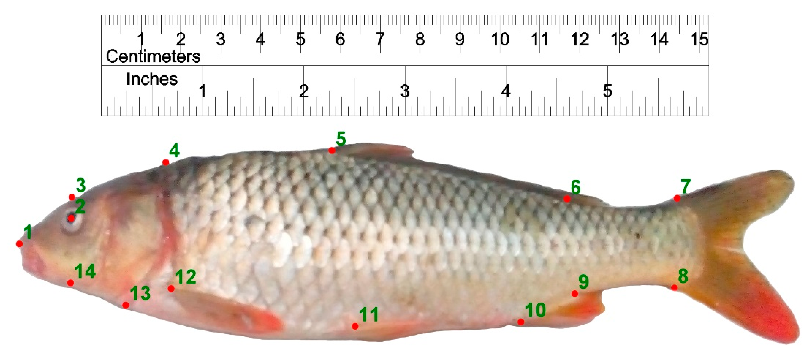
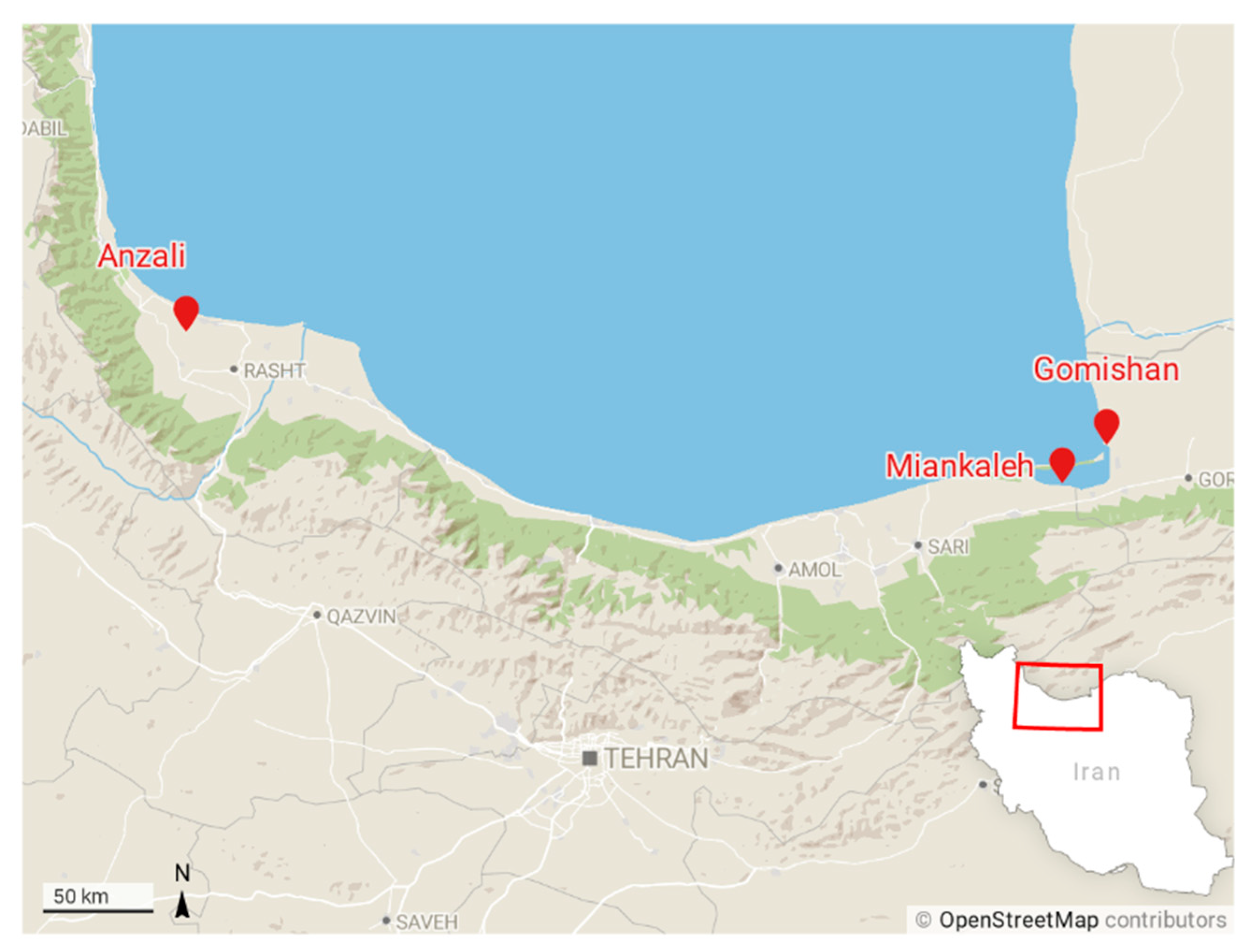
2.1. Sampling
2.2. Data Preparation
2.3. Data Analysis
2.3.1. Attribute Weighting
- Information gain: The relevance of an attribute is evaluated by computing the information gain.
- Information gain ratio: Calculates the correlation of a feature by computing the information gain ratio.
- Weight by rule: The operator calculates the relation of a feature through computing the error rate of a model on the dataset without this attribute.
- Weight by deviation: Weights from the standard deviations of all the features are used by this operator.
- Weight by Chi Squared statistic: This operator quantifies the correlation of a feature by computing for each attribute of the input dataset the value of the chi-squared statistic considering the class attribute.
- Weight by Gini Index: The relevance of a feature is determined by computing the Gini index of the class distribution.
- Weight by Uncertainty: This operator uses the connection of an attribute by measuring the symmetrical uncertainty considering the class distribution.
- Weight by Relief: This operator calculates the relevance of the attributes by relief. The key idea of relief is to estimate the quality of features according to how well their values distinguish between the instances of the same and different classes that are near each other.
- Weight by Support Vector Machine (SVM): The coefficients of the normal vector of a linear SVM are considered as weights of the features.
- Weight by PCA: Factors of the first principal component are used to weight features.
2.3.2. Machine Learning Prediction of Target Populations
Tree Induction
2.3.3. Linear Discriminant Analysis (LDA)
3. Results
3.1. Attribute Weighting (Feature Selection) Models
3.2. Predictions Based on Machine-Learning Algorithms
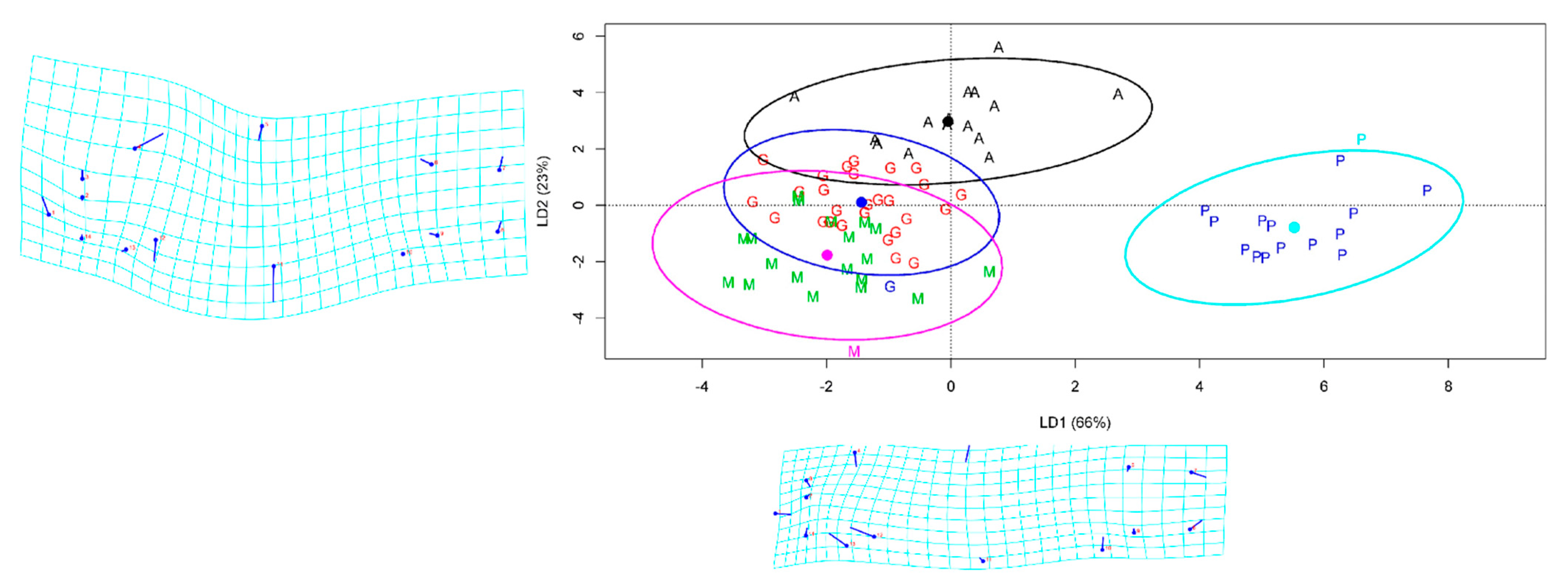
3.3. Linear Discriminant Analysis (LDA)
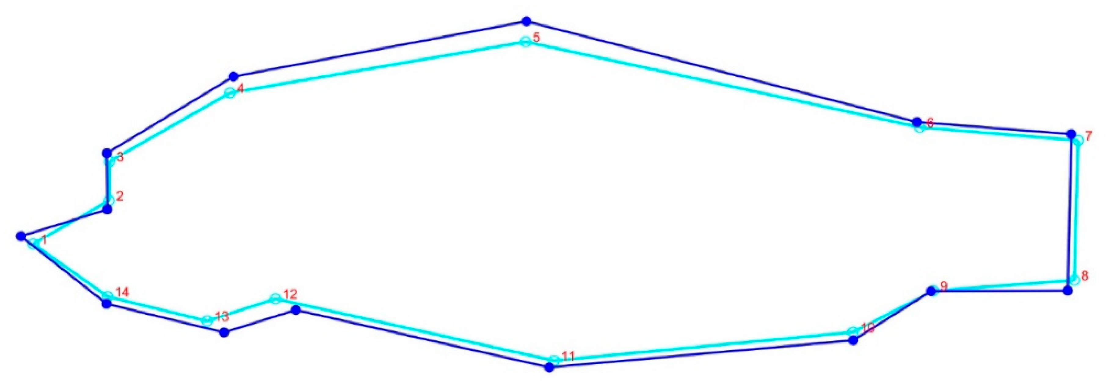
3.4. Geomorph Variations
4. Discussion
5. Conclusions
Supplementary Materials
Author Contributions
Funding
Institutional Review Board Statement
Data Availability Statement
Acknowledgments
Conflicts of Interest
References
- Imoto, J.M.; Saitoh, K.; Sasaki, T.; Yonezawa, T.; Adachi, J.; Kartavtsev, Y.P.; Miya, M.; Nishida, M.; Hanzawa, N. Phylogeny and biogeography of highly diverged freshwater fish species (Leuciscinae, Cyprinidae, Teleostei) inferred from mitochondrial genome analysis. Gene 2013, 514, 112–124. [Google Scholar] [CrossRef] [PubMed]
- Xu, P.; Zhang, X.; Wang, X.; Li, J.; Liu, G.; Kuang, Y.; Xu, J.; Zheng, X.; Ren, L.; Wang, G. Genome sequence and genetic diversity of the common carp, Cyprinus carpio. Nat. Genet. 2014, 46, 1212–1219. [Google Scholar] [CrossRef] [PubMed] [Green Version]
- Kohlmann, K.; Gross, R.; Murakaeva, A.; Kersten, P. Genetic variability and structure of common carp (Cyprinus carpio) populations throughout the distribution range inferred from allozyme, microsatellite and mitochondrial DNA markers. Aquat. Living Resour. 2003, 16, 421–431. [Google Scholar] [CrossRef]
- Akbarzadeh, A.; Farahmand, H.; Shabani, A.; Karami, M.; Kaboli, M.; Abbasi, K.; Rafiee, G. Morphological variation of the pikeperch Sander lucioperca (L.) in the southern Caspian Sea, using a truss system. J. Appl. Ichthyol. 2009, 25, 576–582. [Google Scholar] [CrossRef]
- Ibañez, A.L.; Cowx, I.G.; O’higgins, P. Geometric morphometric analysis of fish scales for identifying genera, species, and local populations within the Mugilidae. Can. J. Fish. Aquat. Sci. 2007, 64, 1091–1100. [Google Scholar] [CrossRef] [Green Version]
- Krpo-Ćetković, J.; Stamenković, S. Morphological differentiation of the pikeperch Stizostedion lucioperca (L.) populations from the Yugoslav part of the Danube. In Proceedings of the Annales Zoologici Fennici, Helsinki, Finland, 28 November 1996; pp. 711–723. [Google Scholar]
- Konstantinidis, I.; Saetrom, P.; Mjelle, R.; Nedoluzhko, A.V.; Robledo, D.; Fernandes, J.M.O. Major gene expression changes and epigenetic remodelling in Nile tilapia muscle after just one generation of domestication. Epigenetics 2020, 15, 1052–1067. [Google Scholar] [CrossRef] [Green Version]
- Podgorniak, T.; Brockmann, S.; Konstantinidis, I.; Fernandes, J.M.O. Differences in the fast muscle methylome provide insight into sex-specific epigenetic regulation of growth in Nile tilapia during early stages of domestication. Epigenetics 2019, 14, 818–836. [Google Scholar] [CrossRef]
- Wilkins, A.S.; Wrangham, R.W.; Fitch, W.T. The “domestication syndrome” in mammals: A unified explanation based on neural crest cell behavior and genetics. Genetics 2014, 197, 795–808. [Google Scholar] [CrossRef] [Green Version]
- Araki, H.; Cooper, B.; Blouin, M.S. Genetic effects of captive breeding cause a rapid, cumulative fitness decline in the wild. Science 2007, 318, 100–103. [Google Scholar] [CrossRef] [Green Version]
- Magnan, P.; Reinbold, D.; Thorgaard, G.H.T.H.; Carter, P.A.C.A. Reduced swimming performance and increased growth in domesticated rainbow trout, Oncorhynchus mykiss. Can. J. Fish. Aquat. Sci. 2009, 66, 1025–1032. [Google Scholar] [CrossRef]
- Hansen, L.P.; Jacobsen, J.A.; Lund, R.A. High numbers of farmed Atlantic salmon. Salmo salar L., observed in oceanic waters north of the Faroe Islands. Aquac. Res. 1993, 24, 777–781. [Google Scholar] [CrossRef]
- Naylor, R.L.; Goldburg, R.J.; Primavera, J.H.; Kautsky, N.; Beveridge, M.C.; Clay, J.; Folke, C.; Lubchenco, J.; Mooney, H.; Troell, M. Effect of aquaculture on world fish supplies. Nature 2000, 405, 1017. [Google Scholar] [CrossRef] [PubMed] [Green Version]
- Ohara, K.; Ariyoshi, T.; Sumida, E.; Sitizyo, K.; Taniguchi, N. Natural hybridization between diploid crucian carp species and genetic independence of triploid crucian carp elucidated by DNA markers. Zool. Sci. 2000, 17, 357–364. [Google Scholar]
- Khalili, K.J.; Amirkolaie, A.K. Comparison of common carp (Cyprinus carpio L.) morphological and electrophoretic characteristics in the southern coast of the Caspian Sea. J. Fish. Aquat. Sci. 2010, 5, 200–207. [Google Scholar] [CrossRef] [Green Version]
- Wang, L.; Shi, X.; Su, Y.; Meng, Z.; Lin, H. Loss of genetic diversity in the cultured stocks of the large yellow croaker, Larimichthys crocea, revealed by microsatellites. Int. J. Mol. Sci. 2012, 13, 5584–5597. [Google Scholar] [CrossRef] [Green Version]
- Johnson, D.; Freiwald, J.; Bernardi, G. Genetic diversity affects the strength of population regulation in a marine fish. Ecology 2016, 97, 627–639. [Google Scholar] [CrossRef]
- Li, L.; Lin, H.; Tang, W.; Liu, D.; Bao, B.; Yang, J. Population genetic structure in wild and aquaculture populations of Hemibarbus maculates inferred from microsatellites markers. Aquac. Fish. 2017, 2, 78–83. [Google Scholar] [CrossRef]
- Zhang, H. The Optimality of Naive Bayes. In Proceedings of the Seventeenth International Florida Artificial Intelligence Research Society Conference, Menlo Park, CA, USA, 12–14 May 2004. [Google Scholar]
- Nasa, C. Evaluation of different classification techniques for web data. Int. J. Comput. Appl. 2012, 52, 34–40. [Google Scholar] [CrossRef]
- Grossman, D.; Domingos, P. Learning Bayesian network classifiers by maximizing conditional likelihood. In Proceedings of the Twenty-first international conference on Machine learning, Banff, AB, Canada, 4–8 July 2004; p. 46. [Google Scholar]
- Lewis, D.D. Naive (Bayes) at forty: The independence assumption in information retrieval. In Proceedings of the European conference on machine learning, Chemnitz, Germany, 21–23 April 1998; pp. 4–15. [Google Scholar]
- Bernardo, J.; Bayarri, M.; Berger, J.; Dawid, A.; Heckerman, D.; Smith, A.; West, M. Bayesian factor regression models in the “large p, small n” paradigm. Bayesian Stat. 2003, 7, 733–742. [Google Scholar]
- Zhao, Y.; Zhang, Y. Comparison of decision tree methods for finding active objects. Adv. Space Res. 2008, 41, 1955–1959. [Google Scholar] [CrossRef] [Green Version]
- Provost, F.; Domingos, P. Tree induction for probability-based ranking. Mach. Learn. 2003, 52, 199–215. [Google Scholar] [CrossRef]
- Kingsford, C.; Salzberg, S.L. What are decision trees? Nat. Biotechnol. 2008, 26, 1011. [Google Scholar] [CrossRef] [PubMed]
- Quinlan, J.R. Induction of decision trees. Mach. Learn. 1986, 1, 81–106. [Google Scholar] [CrossRef] [Green Version]
- Kohavi, R.; Quinlan, J.R. Data mining tasks and methods: Classification: Decision-tree discovery. In Handbook of Data Mining and Knowledge Discovery; Springer: Heidelber/Berlin, Germany, 2002; pp. 267–276. [Google Scholar]
- Guisande, C.; Manjarrés-Hernández, A.; Pelayo-Villamil, P.; Granado-Lorencio, C.; Riveiro, I.; Acuña, A.; Prieto-Piraquive, E.; Janeiro, E.; Matías, J.; Patti, C. IPez: An expert system for the taxonomic identification of fishes based on machine learning techniques. Fish. Res. 2010, 102, 240–247. [Google Scholar] [CrossRef]
- Hnin, T.T.; Lynn, K.T. Fish Classification Based on Robust Features Selection Using Machine Learning Techniques. In Genetic and Evolutionary Computing; Springer: Heidelber/Berlin, Germany, 2016; pp. 237–245. [Google Scholar]
- Zhao, S.; Zhang, S.; Liu, J.; Wang, H.; Zhu, J.; Li, D.; Zhao, R. Application of machine learning in intelligent fish aquaculture: A review. Aquaculture 2021, 540, 736724. [Google Scholar] [CrossRef]
- Abràmoff, M.D.; Magalhães, P.J.; Ram, S.J. Image processing with ImageJ. Biophotonics Int. 2004, 11, 36–42. [Google Scholar]
- Hammer, Ø.; Harper, D.A.; Ryan, P.D. PAST: Paleontological statistics software package for education and data analysis. Palaeontol. Electron. 2001, 4, 9. [Google Scholar]
- Elliott, N.; Haskard, K.; Koslow, J. Morphometric analysis of orange roughy (Hoplostethus atlanticus) off the continental slope of southern Australia. J. Fish Biol. 1995, 46, 202–220. [Google Scholar] [CrossRef]
- Mouludi-Saleh, A.; Eagderi, S.; Cicek, E.; Sungur, S. Morphological variation of Transcaucasian chub, Squalius turcicus in southern Caspian Sea basin using geometric morphometric technique. Biologia 2020, 75, 1585–1590. [Google Scholar] [CrossRef]
- Langley, P. Selection of relevant features in machine learning. In Proceedings of the AAAI Fall symposium on relevance, Monteleone Hotel, New Orleans, LA, USA, 4–6 September 1994; pp. 245–271. [Google Scholar]
- Guyon, I.; Elisseeff, A. An introduction to variable and feature selection. J. Mach. Learn. Res. 2003, 3, 1157–1182. [Google Scholar]
- Ebrahimie, E.; Ebrahimi, M.; Sarvestani, N.R.; Ebrahimi, M. Protein attributes contribute to halo-stability, bioinformatics approach. Saline Syst. 2011, 7, 1. [Google Scholar] [CrossRef] [PubMed] [Green Version]
- Ebrahimi, M.; Lakizadeh, A.; Agha-Golzadeh, P.; Ebrahimie, E.; Ebrahimi, M. Prediction of thermostability from amino acid attributes by combination of clustering with attribute weighting: A new vista in engineering enzymes. PLoS ONE 2011, 6, e23146. [Google Scholar] [CrossRef] [PubMed] [Green Version]
- Ebrahimi, M.; Mohammadi-Dehcheshmeh, M.; Ebrahimie, E.; Petrovski, K.R. Comprehensive analysis of machine learning models for prediction of sub-clinical mastitis: Deep Learning and Gradient-Boosted Trees outperform other models. Comput. Biol. Med. 2019, 114, 103456. [Google Scholar] [CrossRef] [PubMed]
- Shekoofa, A.; Emam, Y.; Shekoufa, N.; Ebrahimi, M.; Ebrahimie, E. Determining the most important physiological and agronomic traits contributing to maize grain yield through machine learning algorithms: A new avenue in intelligent agriculture. PLoS ONE 2014, 9, e97288. [Google Scholar] [CrossRef] [Green Version]
- Bakhtiarizadeh, M.R.; Moradi-Shahrbabak, M.; Ebrahimi, M.; Ebrahimie, E. Neural network and SVM classifiers accurately predict lipid binding proteins, irrespective of sequence homology. J. Theor. Biol. 2014, 356, 213–222. [Google Scholar] [CrossRef]
- Hosseinzadeh, F.; Ebrahimi, M.; Goliaei, B.; Shamabadi, N. Classification of lung cancer tumors based on structural and physicochemical properties of proteins by bioinformatics models. PLoS ONE 2012, 7, e40017. [Google Scholar] [CrossRef]
- Beiki, A.H.; Saboor, S.; Ebrahimi, M. A new avenue for classification and prediction of olive cultivars using supervised and unsupervised algorithms. PLoS ONE 2012, 7, e44164. [Google Scholar] [CrossRef] [Green Version]
- Larson, W.A.; Seeb, L.W.; Everett, M.V.; Waples, R.K.; Templin, W.D.; Seeb, J.E. Genotyping by sequencing resolves shallow population structure to inform conservation of Chinook salmon (Oncorhynchus tshawytscha). Evol. Appl. 2014, 7, 355–369. [Google Scholar] [CrossRef]
- Torkzaban, B.; Kayvanjoo, A.H.; Ardalan, A.; Mousavi, S.; Mariotti, R.; Baldoni, L.; Ebrahimie, E.; Ebrahimi, M.; Hosseini-Mazinani, M. Machine learning based classification of microsatellite variation: An effective approach for phylogeographic characterization of olive populations. PLoS ONE 2015, 10, e0143465. [Google Scholar]
- Anastasiadi, D.; Piferrer, F. Epimutations in developmental genes underlie the onset of domestication in farmed European sea bass. Mol. Biol. Evol. 2019, 36, 2252–2264. [Google Scholar] [CrossRef]
- Pulcini, D.; Wheeler, P.; Cataudella, S.; Russo, T.; Thorgaard, G. Domestication shapes morphology in rainbow trout Oncorhynchus mykiss. J. Fish Biol. 2013, 82, 390–407. [Google Scholar] [CrossRef] [PubMed]
- Zeng, L.; Zhou, L.; Guo, D.L.; Fu, D.H.; Xu, P.; Zeng, S.; Tang, Q.D.; Chen, A.L.; Chen, F.Q.; Luo, Y. Ecological effects of dams, alien fish, and physiochemical environmental factors on homogeneity/heterogeneity of fish community in four tributaries of the Pearl River in China. Ecol. Evol. 2017, 7, 3904–3915. [Google Scholar] [CrossRef] [PubMed]
- Akbari, M.; Baubekova, A.; Roozbahani, A.; Gafurov, A.; Shiklomanov, A.; Rasouli, K.; Ivkina, N.; Kløve, B.; Haghighi, A.T. Vulnerability of the Caspian Sea shoreline to changes in hydrology and climate. Environ. Res. Lett. 2020, 15, 115002. [Google Scholar] [CrossRef]
- Crétaux, J.-F.; Jelinski, W.; Calmant, S.; Kouraev, A.; Vuglinski, V.; Bergé-Nguyen, M.; Gennero, M.-C.; Nino, F.; Del Rio, R.A.; Cazenave, A. SOLS: A lake database to monitor in the Near Real Time water level and storage variations from remote sensing data. Adv. Space Res. 2011, 47, 1497–1507. [Google Scholar] [CrossRef]
- Jafari, O.; Zeinalabedini, M.; Robledo, D.; Fernandes, J.M.D.O.; Hedayati, A.A.; Babak, A. Genotyping-by-Sequencing Reveals the Impact of Restocking on Wild Common Carp Populations of the Southern Caspian Basin. Front. Ecol. Evol. 2022, 10, 872176. [Google Scholar] [CrossRef]
- Ebrahimie, E.; Ebrahimi, M.; Ebrahimi, M. Searching for patterns of thermostability in proteins and defining the main features contributing to enzyme thermostability through screening, clustering, and decision tree algorithms. EXCLI J. 2010, 8, 218–233. [Google Scholar]
- Jafari, O.; Fernandes, J.M.D.O.; Hedayati, A.-A.; Shabany, A.; Nasrolahpourmoghadam, M. Microsatellite analysis of five populations of Alosa braschnikowi (Borodin, 1904) across the southern coast of the Caspian Sea. Front. Genet. 2019, 10, 760. [Google Scholar] [CrossRef] [Green Version]
- Banan, A.; Nasiri, A.; Taheri-Garavand, A. Deep learning-based appearance features extraction for automated carp species identification. Aquac. Eng. 2020, 89, 102053. [Google Scholar] [CrossRef]
- Kutlu, Y.; Altan, G.; İşçimen, B.; Doğdu, S.A.; Turan, C. Recognition of species of triglidae family using deep learning. J. Black Sea/Mediterr. Environ. 2017, 23, 56–65. [Google Scholar]
- Courtenay, L.A.; Huguet, R.; González-Aguilera, D.; Yravedra, J. A hybrid geometric morphometric deep learning approach for cut and trampling mark classification. Appl. Sci. 2020, 10, 150. [Google Scholar] [CrossRef] [Green Version]


| PCA | SVM | Relief | Uncertainty | Gini Index | Chi-Squared | Deviation | Rule | Info Gain Ratio | Info Gain | Attribute | Count Weights > 0.7 |
|---|---|---|---|---|---|---|---|---|---|---|---|
| 0.85 | 0.45 | 0.87 | 0.83 | 1.00 | 0.76 | 0.76 | 0.42 | 1.00 | 1.00 | HH1 | 8 |
| 0.44 | 0.49 | 0.91 | 0.82 | 0.77 | 0.91 | 0.43 | 1.00 | 0.81 | 0.73 | PelH | 7 |
| 0.54 | 0.36 | 1.00 | 1.00 | 0.76 | 1.00 | 0.42 | 0.04 | 0.68 | 0.98 | POL | 5 |
| 1.00 | 0.08 | 0.55 | 0.77 | 0.70 | 0.75 | 1.00 | 0.31 | 0.54 | 0.76 | HL | 5 |
| 0.48 | 0.23 | 0.47 | 0.70 | 0.77 | 0.70 | 0.62 | 1.00 | 0.81 | 0.65 | PH | 5 |
| 0.23 | 0.33 | 0.70 | 0.67 | 0.78 | 0.65 | 0.15 | 0.46 | 0.79 | 0.80 | CPH | 3 |
| Attribute (Landmarks) | Weight_ Info Gain | Weight_Info Gain Ratio | Weight_Rule | Weight_Deviation | Weight_Chi Squared | Weight_Gini Index | Weight_ Uncertainty | Weight_Relief | Weight_SVM | Weight_PCA | Count Weights > 0.7 |
|---|---|---|---|---|---|---|---|---|---|---|---|
| L12 | 1.0 | 1.0 | 0 | 0.6 | 1.0 | 1.0 | 1.0 | 1.0 | 1.0 | 0.6 | 7 |
| L5 | 0.7 | 0.3 | 1.0 | 1.0 | 0.9 | 0.6 | 0.9 | 0.4 | 0.5 | 1.0 | 5 |
| L13 | 0.8 | 0.7 | 1.0 | 0.4 | 0.6 | 0.7 | 0.6 | 0.5 | 0.8 | 0.4 | 4 |
| L7 | 0.4 | 0.9 | 1.0 | 0.4 | 0.5 | 0.4 | 0.4 | 0.4 | 0.4 | 0.4 | 2 |
| L1 | 0.4 | 0.4 | 1.0 | 0.5 | 0.5 | 0.5 | 0.6 | 0.5 | 0 | 0.4 | 1 |
| L8 | 0.3 | 0.3 | 1.0 | 0.4 | 0.1 | 0.2 | 0.2 | 0.2 | 0.4 | 0.3 | 1 |
| L3 | 0.4 | 0.4 | 1.0 | 0.0 | 0.2 | 0.4 | 0.3 | 0.2 | 0.2 | 0.1 | 1 |
| L2 | 0.4 | 0.2 | 1.0 | 0.0 | 0.2 | 0.4 | 0.2 | 0.1 | 0.5 | 0 | 1 |
| L9 | 0.2 | 0.1 | 1.0 | 0.3 | 0.1 | 0.2 | 0.1 | 0.3 | 0.5 | 0 | 1 |
| L4 | 0.1 | 0.1 | 1.0 | 0.4 | 0.1 | 0.1 | 0.2 | 0 | 0.1 | 0.3 | 1 |
| L11 | 0.1 | 0.3 | 0 | 0.6 | 0.1 | 0.1 | 0.2 | 0.1 | 0.4 | 0 | 0 |
| L10 | 0 | 0 | 1.0 | 0.2 | 0 | 0 | 0 | 0 | 0.6 | 0 | 1 |
| L14 | 0.1 | 0.5 | 1.0 | 0.1 | 0.1 | 0.1 | 0 | 0 | 0.1 | 0 | 1 |
| L6 | 0.1 | 0.1 | 0 | 0.4 | 0 | 0.2 | 0 | 0.1 | 0.4 | 0.1 | 0 |
| Database | |||||||||||
|---|---|---|---|---|---|---|---|---|---|---|---|
| DT Algorithms | Chi-Squared | Info Gain | Deviation | Gini Index | Info Gain Ratio | PCA | Relief | Rule | Uncertainty | FCDB | SVM |
| DT Random Forest Accuracy | 0.65 | 0.56 | 0.55 | 0.61 | 0.54 | 0.6 | 0.56 | 0.48 | 0.53 | 0.51 | 0.52 |
| DT Random Forest Gain Ratio | 0.52 | 0.64 | 0.49 | 0.57 | 0.51 | 0.63 | 0.6 | 0.55 | 0.58 | 0.59 | 0.4 |
| DT Random Forest Gini Index | 0.59 | 0.58 | 0.59 | 0.71 | 0.51 | 0.54 | 0.53 | 0.5 | 0.53 | 0.56 | 0.5 |
| DT Random Forest Info Gain | 0.61 | 0.57 | 0.54 | 0.64 | 0.56 | 0.51 | 0.58 | 0.51 | 0.61 | 0.54 | 0.41 |
| Max Performance | 0.65 | 0.64 | 0.59 | 0.71 | 0.56 | 0.63 | 0.6 | 0.55 | 0.61 | 0.59 | 0.52 |
| DT Stump Accuracy | 0.53 | 0.5 | 0.54 | 0.5 | 0.5 | 0.54 | 0.53 | 0.5 | 0.53 | 0.5 | 0.52 |
| DT Stump Gain Ratio | 0.56 | 0.56 | 0.59 | 0.56 | 0.56 | 0.56 | 0.56 | 0.59 | 0.56 | 0.56 | 0.43 |
| DT Stump Gini Index | 0.57 | 0.57 | 0.57 | 0.57 | 0.57 | 0.57 | 0.57 | 0.57 | 0.57 | 0.57 | 0.51 |
| DT Stump Info Gain | 0.51 | 0.51 | 0.54 | 0.51 | 0.51 | 0.51 | 0.51 | 0.57 | 0.51 | 0.51 | 0.51 |
| Max Performance | 0.57 | 0.57 | 0.59 | 0.57 | 0.57 | 0.57 | 0.57 | 0.59 | 0.57 | 0.57 | 0.52 |
| DT Parallel Accuracy | 0.6 | 0.61 | 0.74 | 0.65 | 0.65 | 0.62 | 0.62 | 0.77 | 0.74 | 0.66 | 0.51 |
| DT Parallel Gain Ratio | 0.65 | 0.63 | 0.6 | 0.59 | 0.66 | 0.64 | 0.65 | 0.71 | 0.67 | 0.61 | 0.54 |
| DT Parallel Gini Index | 0.66 | 0.7 | 0.67 | 0.65 | 0.71 | 0.63 | 0.62 | 0.71 | 0.66 | 0.65 | 0.58 |
| DT Parallel Info Gain | 0.68 | 0.65 | 0.62 | 0.74 | 0.63 | 0.58 | 0.63 | 0.62 | 0.67 | 0.73 | 0.56 |
| Max Performance | 0.68 | 0.7 | 0.74 | 0.74 | 0.71 | 0.64 | 0.65 | 0.77 | 0.74 | 0.73 | 0.58 |
| Decision Tree Accuracy | 0.65 | 0.68 | 0.66 | 0.68 | 0.65 | 0.61 | 0.66 | 0.72 | 0.71 | 0.74 | 0.51 |
| Decision Tree Gain Ratio | 0.62 | 0.59 | 0.6 | 0.59 | 0.64 | 0.57 | 0.6 | 0.57 | 0.6 | 0.59 | 0.42 |
| Decision Tree Gini Index | 0.61 | 0.66 | 0.6 | 0.66 | 0.56 | 0.59 | 0.63 | 0.7 | 0.65 | 0.68 | 0.44 |
| Decision Tree Info Gain | 0.64 | 0.56 | 0.61 | 0.56 | 0.59 | 0.55 | 0.61 | 0.58 | 0.59 | 0.54 | 0.41 |
| Max Performance | 0.65 | 0.68 | 0.66 | 0.68 | 0.65 | 0.61 | 0.66 | 0.72 | 0.71 | 0.74 | 0.51 |
| Dataset | Geometric Morphometric | Traditional Morphometric | ||
|---|---|---|---|---|
| Bayes Kernel | Naïve Bayes | Bayes Kernel | Naïve Bayes | |
| Rule | 0.36 | 0.43 | 0.64 | 0.73 |
| SVM | 0.36 | 0.53 | 0.42 | 0.52 |
| Uncertainty | 0.36 | 0.46 | 0.64 | 0.71 |
| Relief | 0.36 | 0.47 | 0.64 | 0.68 |
| PCA | 0.36 | 0.47 | 0.62 | 0.61 |
| Info Gain Ratio | 0.36 | 0.54 | 0.55 | 0.61 |
| Info Gain | 0.36 | 0.47 | 0.63 | 0.68 |
| Gini Index | 0.36 | 0.47 | 0.57 | 0.64 |
| Deviation | 0.36 | 0.52 | 0.64 | 0.64 |
| Chi-Squared | 0.36 | 0.46 | 0.64 | 0.69 |
| FCDB | 0.40 | 0.60 | 0.70 | 0.77 |
| Predicted Anzali | Predicted Gomishan | Predicted Miankaleh | Predicted Farmed | Precision (%) | |
|---|---|---|---|---|---|
| Actual Anzali | 7 | 4 | 2 | 1 | 50.0 |
| Actual Gomishan | 1 | 23 | 3 | 0 | 85.2 |
| Actual Minkaleh | 0 | 3 | 16 | 0 | 84.2 |
| Actual Farmed | 0 | 0 | 0 | 14 | 100.0 |
| Recall (%) | 87.5 | 76.7 | 76.2 | 93.3 | |
| Overall Accuracy: 81.1% | |||||
Publisher’s Note: MDPI stays neutral with regard to jurisdictional claims in published maps and institutional affiliations. |
© 2022 by the authors. Licensee MDPI, Basel, Switzerland. This article is an open access article distributed under the terms and conditions of the Creative Commons Attribution (CC BY) license (https://creativecommons.org/licenses/by/4.0/).
Share and Cite
Jafari, O.; Ebrahimi, M.; Hedayati, S.A.-A.; Zeinalabedini, M.; Poorbagher, H.; Nasrolahpourmoghadam, M.; Fernandes, J.M.O. Integration of Morphometrics and Machine Learning Enables Accurate Distinction between Wild and Farmed Common Carp. Life 2022, 12, 957. https://doi.org/10.3390/life12070957
Jafari O, Ebrahimi M, Hedayati SA-A, Zeinalabedini M, Poorbagher H, Nasrolahpourmoghadam M, Fernandes JMO. Integration of Morphometrics and Machine Learning Enables Accurate Distinction between Wild and Farmed Common Carp. Life. 2022; 12(7):957. https://doi.org/10.3390/life12070957
Chicago/Turabian StyleJafari, Omid, Mansour Ebrahimi, Seyed Ali-Akbar Hedayati, Mehrshad Zeinalabedini, Hadi Poorbagher, Maryam Nasrolahpourmoghadam, and Jorge M. O. Fernandes. 2022. "Integration of Morphometrics and Machine Learning Enables Accurate Distinction between Wild and Farmed Common Carp" Life 12, no. 7: 957. https://doi.org/10.3390/life12070957
APA StyleJafari, O., Ebrahimi, M., Hedayati, S. A.-A., Zeinalabedini, M., Poorbagher, H., Nasrolahpourmoghadam, M., & Fernandes, J. M. O. (2022). Integration of Morphometrics and Machine Learning Enables Accurate Distinction between Wild and Farmed Common Carp. Life, 12(7), 957. https://doi.org/10.3390/life12070957