Paleozoic–Mesozoic Eustatic Changes and Mass Extinctions: New Insights from Event Interpretation


Abstract

1. Introduction
2. Methodology
3. Results
4. Discussion
5. Conclusions
Supplementary Materials
Funding
Acknowledgments
Conflicts of Interest
References
- Bambach, R.K. Phanerozoic biodiversity mass extinctions. Annu. Rev. Earth Planet. Sci. 2006, 34, 127–155. [Google Scholar] [CrossRef]
- Benton, M.J. The evolutionary significance of mass extinctions. Trends Ecol. Evol. 1986, 1, 127–130. [Google Scholar] [CrossRef]
- Benton, M.J. Diversification and extinction in the history of life. Science 1995, 268, 52–58. [Google Scholar] [CrossRef]
- Clapham, M.E.; Renne, P.R. Flood basalts and mass extinctions. Annu. Rev. Earth Planet. Sci. 2019, 47, 275–303. [Google Scholar] [CrossRef]
- Elewa, A.M.T.; Abdelhady, A.A. Past, present, and future mass extinctions. J. Afr. Earth Sci. 2020, 162, 103678. [Google Scholar] [CrossRef]
- Erwin, D.H. The end and the beginning: Recoveries from mass extinctions. Trends Ecol. Evol. 1998, 13, 344–349. [Google Scholar] [CrossRef]
- Hallam, A. Mass extinctions in Phanerozoic time. Geol. Soc. Spec. Publ. 1998, 140, 259–274. [Google Scholar] [CrossRef]
- Holland, S.M. The Stratigraphy of Mass Extinctions and Recoveries. Annu. Rev. Earth Planet. Sci. 2020, 48, 75–97. [Google Scholar] [CrossRef]
- Jablonski, D. Mass extinctions and macroevolution. Paleobiology 2005, 31, 192–210. [Google Scholar] [CrossRef]
- Melott, A.L.; Bambach, R.K. Analysis of periodicity of extinction using the 2012 geological timescale. Paleobiology 2014, 40, 177–196. [Google Scholar] [CrossRef]
- Racki, G. The Alvarez impact theory of mass extinction; limits to its applicability and the “great expectations syndrome”. Acta Palaeontol. Pol. 2012, 57, 681–702. [Google Scholar] [CrossRef]
- Rampino, M.R.; Caldeira, K. Periodic impact cratering and extinction events over the last 260 million years. Mon. Not. R. Astron. Soc. 2015, 454, 3480–3484. [Google Scholar] [CrossRef]
- Raup, D.M.; Sepkoski, J.J., Jr. Mass extinctions in the marine fossil record. Science 1982, 215, 1501–1503. [Google Scholar] [CrossRef] [PubMed]
- Thomas, E. Cenozoic mass extinctions in the deep sea: What perturbs the largest habitat on Earth? Spec. Pap. Geol. Soc. Am. 2004, 424, 1–23. [Google Scholar]
- Twitchett, R.J. The palaeoclimatology, palaeoecology and palaeoenvironmental analysis of mass extinction events. Palaeogeogr. Palaeoclimatol. Palaeoecol. 2006, 232, 190–213. [Google Scholar] [CrossRef]
- Wignall, P.B. Large igneous provinces and mass extinctions. Earth-Sci. Rev. 2001, 53, 1–33. [Google Scholar] [CrossRef]
- Hallam, A.; Wignall, P.B. Mass extinctions and sea-level changes. Earth Sci. Rev. 1999, 48, 217–250. [Google Scholar] [CrossRef]
- Newell, N.D. Revolutions in the history of life. Geol. Soc. Am. Spec. Pap. 1967, 89, 63–91. [Google Scholar]
- Peters, S.E.; Foote, M. Biodiversity in the Phanerozoic: A reinterpretation. Paleobiology 2001, 27, 583–600. [Google Scholar] [CrossRef]
- Roberts, G.G.; Mannion, P.D. Timing and periodicity of Phanerozoic marine biodiversity and environmental change. Sci. Rep. 2019, 9, 6116. [Google Scholar] [CrossRef]
- Smith, A.B. Large-scale heterogeneity of the fossil record: Implications for Phanerozoic biodiversity studies. Philos. Trans. R. Soc. B Biol. Sci. 2001, 356, 351–367. [Google Scholar] [CrossRef] [PubMed]
- Ruban, D.A. A “chaos” of Phanerozoic eustatic curves. J. Afr. Earth Sci. 2016, 116, 225–232. [Google Scholar] [CrossRef]
- Ruban, D.A. Unawareness and Theorizing in Modern Geology: Two Examples Based on Citation Analysis. Earth 2020, 1, 1–14. [Google Scholar] [CrossRef]
- Raup, D.M.; Sepkoski, J.J., Jr. Periodicity of extinctions in the geologic past. Proc. Natl. Acad. Sci. USA 1984, 81, 801–805. [Google Scholar] [CrossRef]
- Raup, D.M.; Sepkoski, J.J., Jr. Periodic extinction of families and genera. Science 1986, 231, 833–836. [Google Scholar] [CrossRef]
- Boulila, S.; Laskar, J.; Haq, B.U.; Galbrun, B.; Hara, N. Long-term cyclicities in Phanerozoic sea-level sedimentary record and their potential drivers. Glob. Planet. Chang. 2018, 165, 128–136. [Google Scholar] [CrossRef]
- Gillman, M.P.; Erenler, H.E. Globally disruptive events show predictable timing patterns. Int. J. Astrobiol. 2016, 16, 91–96. [Google Scholar] [CrossRef]
- Lipowski, A. Periodicity of mass extinctions without an extraterrestrial cause. Phys. Rev. E Stat. Nonlinear Soft Matter Phys. 2005, 71, 052902. [Google Scholar] [CrossRef]
- McKinney, M.L. Periodic mass extinctions: Product of biosphere growth dynamics? Hist. Biol. 1989, 2, 273–287. [Google Scholar] [CrossRef]
- Rampino, M.R. Relationship between impact-crater size and severity of related extinction episodes. Earth Sci. Rev. 2020, 201, 102990. [Google Scholar] [CrossRef]
- Tiwari, R.K.; Rao, K.N.N. Mega geocycles: Echoes of astronomical events. J. Geol. Soc. India 2003, 62, 181–190. [Google Scholar]
- Haq, B.U. Cretaceous eustasy revisited. Glob. Planet. Chang. 2014, 113, 44–58. [Google Scholar] [CrossRef]
- Haq, B.U. Jurassic sea-level variations: A reappraisal. Gsa Today 2018, 28, 4–10. [Google Scholar] [CrossRef]
- Haq, B.U. Triassic eustatic variations reexamined. Gsa Today 2018, 28, 4–9. [Google Scholar] [CrossRef]
- Haq, B.U.; Schutter, S.R. A chronology of Paleozoic sea-level changes. Science 2008, 322, 64–68. [Google Scholar] [CrossRef]
- Haq, B.U.; Al-Qahtani, A.M. Phanerozoic cycles of sea-level change on the Arabian platform. GeoArabia 2005, 10, 127–160. [Google Scholar]
- Haq, B.U.; Hardenbol, J.; Vail, P.R. Chronology of fluctuating sea levels since the Triassic. Science 1987, 235, 1156–1167. [Google Scholar] [CrossRef]
- Ruban, D.A. Episodic events in long-term geological processes: A new classification and its applications. Geosci. Front. 2018, 9, 377–389. [Google Scholar] [CrossRef]
- International Commission on Stratigraphy (ICS). International Chronostratigraphic Chart, v2020/01. Available online: https://stratigraphy.org/icschart/ChronostratChart2020-01.pdf (accessed on 15 October 2020).
- Babcock, L.E.; Peng, S.-C.; Brett, C.E.; Zhu, M.-Y.; Ahlberg, P.; Bevis, M.; Robinson, R.A. Global climate, sea level cycles, and biotic events in the Cambrian Period. Palaeoworld 2015, 24, 5–15. [Google Scholar] [CrossRef]
- Ling, M.-X.; Zhan, R.-B.; Wang, G.-X.; Wang, Y.; Amelin, Y.; Tang, P.; Liu, J.-B.; Jin, J.; Huang, B.; Wu, R.-C.; et al. An extremely brief end Ordovician mass extinction linked to abrupt onset of glaciation. Solid Earth Sci. 2020, 4, 190–198. [Google Scholar] [CrossRef]
- Wang, G.; Zhan, R.; Percival, I.G. The end-Ordovician mass extinction: A single-pulse event? Earth Sci. Rev. 2019, 192, 15–33. [Google Scholar] [CrossRef]
- Lehnert, O.; Männik, P.; Joachimski, M.M.; Calner, M.; Frýda, J. Palaeoclimate perturbations before the Sheinwoodian glaciation: A trigger for extinctions during the ‘Ireviken Event’. Palaeogeogr. Palaeoclimatol. Palaeoecol. 2010, 296, 320–331. [Google Scholar] [CrossRef]
- Racki, G. A volcanic scenario for the Frasnian–Famennian major biotic crisis and other Late Devonian global changes: More answers than questions? Glob. Planet. Chang. 2020, 189, 103174. [Google Scholar] [CrossRef]
- Balseiro, D.; Powell, M.G. Carbonate collapse and the late Paleozoic ice age marine biodiversity crisis. Geology 2020, 48, 118–122. [Google Scholar] [CrossRef]
- McGhee, G.R.; Clapham, M.E.; Sheehan, P.M.; Bottjer, D.J.; Droser, M.L. A new ecological-severity ranking of major Phanerozoic biodiversity crises. Palaeogeogr. Palaeoclimatol. Palaeoecol. 2013, 370, 260–270. [Google Scholar] [CrossRef]
- Arefifard, S.; Payne, J.L. End-Guadalupian extinction of larger fusulinids in central Iran and implications for the global biotic crisis. Palaeogeogr. Palaeoclimatol. Palaeoecol. 2020, 550, 109743. [Google Scholar] [CrossRef]
- Rampino, M.R.; Shen, S.-Z. The end-Guadalupian (259.8 Ma) biodiversity crisis: The sixth major mass extinction? Hist. Biol. 2019. [Google Scholar] [CrossRef]
- Rampino, M.R.; Eshet-Alkalai, Y.; Koutavas, A.; Rodriguez, S. End-Permian stratigraphic timeline applied to the timing of marine and non-marine extinctions. Palaeoworld 2020, 29, 577–589. [Google Scholar] [CrossRef]
- Shen, S.-Z.; Ramezani, J.; Chen, J.; Cao, C.-Q.; Erwin, D.H.; Zhang, H.; Xiang, L.; Schoepfer, S.D.; Henderson, C.M.; Zheng, Q.-F.; et al. A sudden end-Permian mass extinction in South China. Bull. Geol. Soc. Am. 2019, 131, 205–223. [Google Scholar] [CrossRef]
- Song, H.; Wignall, P.B.; Tong, J.; Yin, H. Two pulses of extinction during the Permian-Triassic crisis. Nat. Geosci. 2013, 6, 52–56. [Google Scholar] [CrossRef]
- Ruban, D.A. Examining the Ladinian crisis in light of the current knowledge of the Triassic biodiversity changes. Gondwana Res. 2017, 48, 285–291. [Google Scholar] [CrossRef]
- Dal Corso, J.; Bernardi, M.; Sun, Y.; Song, H.; Seyfullah, L.J.; Preto, N.; Gianolla, P.; Ruffell, A.; Kustatscher, E.; Roghi, G.; et al. Extinction and dawn of the modern world in the Carnian (Late Triassic). Sci. Adv. 2020, 6, eaba0099. [Google Scholar] [CrossRef] [PubMed]
- Rigo, M.; Onoue, T.; Tanner, L.H.; Lucas, S.G.; Godfrey, L.; Katz, M.E.; Zaffani, M.; Grice, K.; Cesar, J.; Yamashita, D.; et al. The Late Triassic Extinction at the Norian/Rhaetian boundary: Biotic evidence and geochemical signature. Earth Sci. Rev. 2020, 204, 103180. [Google Scholar] [CrossRef]
- Tegner, C.; Marzoli, A.; McDonald, I.; Youbi, N.; Lindström, S. Platinum-group elements link the end-Triassic mass extinction and the Central Atlantic Magmatic Province. Sci. Rep. 2020, 10, 3482. [Google Scholar] [CrossRef]
- Wignall, P.B.; Atkinson, J.W. A two-phase end-Triassic mass extinction. Earth Sci. Rev. 2020, 208, 103282. [Google Scholar] [CrossRef]
- Ait-Itto, F.-Z.; Martinez, M.; Price, G.D.; Ait Addi, A. Synchronization of the astronomical time scales in the Early Toarcian: A link between anoxia, carbon-cycle perturbation, mass extinction and volcanism. Earth Planet. Sci. Lett. 2018, 493, 1–11. [Google Scholar] [CrossRef]
- Caruthers, A.H.; Smith, P.L.; Gröcke, D.R. The Pliensbachian-Toarcian (Early Jurassic) extinction: A North American perspective. Spec. Pap. Geol. Soc. Am. 2014, 505, 225–243. [Google Scholar]
- Ruebsam, W.; Reolid, M.; Marok, A.; Schwark, L. Drivers of benthic extinction during the early Toarcian (Early Jurassic) at the northern Gondwana paleomargin: Implications for paleoceanographic conditions. Earth Sci. Rev. 2020, 203, 103117. [Google Scholar] [CrossRef]
- Hallam, A. The Pliensbachian and Tithonian extinction events. Nature 1986, 319, 765–768. [Google Scholar] [CrossRef]
- Ruban, D.A. Diversity dynamics of Callovian-Albian brachiopods in the Northern Caucasus (Northern Neo-Tethys) and a Jurassic/Cretaceous mass extinction. Paleontol. Res. 2011, 15, 154–167. [Google Scholar] [CrossRef]
- Freymueller, N.A.; Moore, J.R.; Myers, C.E. An analysis of the impacts of Cretaceous oceanic anoxic events on global molluscan diversity dynamics. Paleobiology 2019, 45, 280–295. [Google Scholar] [CrossRef]
- Hart, M.B. The ’Black Band’: Local expression of a global event. Proc. Yorks. Geol. Soc. 2018, 62, 217–226. [Google Scholar] [CrossRef]
- Kuroda, J.; Ogawa, N.O.; Tanimizu, M.; Coffin, M.F.; Tokuyama, H.; Kitazato, H.; Ohkouchi, N. Contemporaneous massive subaerial volcanism and late cretaceous Oceanic Anoxic Event 2. Earth Planet. Sci. Lett. 2007, 256, 211–223. [Google Scholar] [CrossRef]
- Schoene, B.; Eddy, M.P.; Samperton, K.M.; Keller, C.B.; Keller, G.; Adatte, T.; Khadri, S.F.R. U-Pb constraints on pulsed eruption of the Deccan Traps across the end-Cretaceous mass extinction. Science 2019, 363, 862–866. [Google Scholar] [CrossRef]
- Faggetter, L.E.; Wignall, P.B.; Pruss, S.B.; Newton, R.J.; Sun, Y.; Crowley, S.F. Trilobite extinctions, facies changes and the ROECE carbon isotope excursion at the Cambrian Series 2–3 boundary, Great Basin, western USA. Palaeogeogr. Palaeoclimatol. Palaeoecol. 2017, 478, 53–66. [Google Scholar] [CrossRef]
- Guo, Q.; Strauss, H.; Liu, C.; Zhao, Y.; Yang, X.; Peng, J.; Yang, H. A negative carbon isotope excursion defines the boundary from Cambrian Series 2 to Cambrian Series 3 on the Yangtze Platform, South China. Palaeogeogr. Palaeoclimatol. Palaeoecol. 2010, 285, 143–151. [Google Scholar] [CrossRef]
- Brenchley, P.J.; Carden, G.A.F.; Marshall, J.D. Environmental changes associated with the "first strike’ of the late Ordovician mass extinction. Mod. Geol. 1995, 20, 69–82. [Google Scholar]
- Sheehan, P.M. The late Ordovician mass-extinction. Annu. Rev. Earth Planet. Sci. 2001, 29, 331–364. [Google Scholar] [CrossRef]
- Sutcliffe, O.E.; Dowdeswell, J.A.; Whittington, R.J.; Theron, J.N.; Craig, J. Calibrating the Late Ordovician glaciation and mass extinction by the eccentricity cycles of Earth’s orbit. Geology 2000, 28, 967–970. [Google Scholar] [CrossRef]
- Eriksson, M.E. The Silurian Ireviken Event and vagile benthic faunal turnovers (Polychaeta; Eunicida) on Gotland, Sweden. GFF 2006, 128, 91–95. [Google Scholar] [CrossRef]
- Jeppsson, L.; Aldridge, R.J.; Dorning, K.J. Wenlock (Silurian) oceanic episodes and events. J. Geol. Soc. 1995, 152, 487–498. [Google Scholar] [CrossRef]
- Johnson, M.E. Relationship of Silurian sea-level fluctuations to oceanic episodes and events. GFF 2006, 128, 115–121. [Google Scholar] [CrossRef]
- Munnecke, A.; Samtleben, C.; Bickert, T. The Ireviken Event in the lower Silurian of Gotland, Sweden—Relation to similar Palaeozoic and Proterozoic events. Palaeogeogr. Palaeoclimatol. Palaeoecol. 2003, 195, 99–124. [Google Scholar] [CrossRef]
- Bond, D.P.G.; Wignall, P.B. The role of sea-level change and marine anoxia in the Frasnian-Famennian (Late Devonian) mass extinction. Palaeogeogr. Palaeoclimatol. Palaeoecol. 2008, 263, 107–118. [Google Scholar] [CrossRef]
- McGhee, G.R. The Late Devonian (Frasnian/Famenian) mass extinction: A proposed test of the glaciation hypothesis. Geol. Q. 2014, 58, 263–268. [Google Scholar] [CrossRef][Green Version]
- De Vleeschouwer, D.; Da Silva, A.-C.; Sinnesael, M.; Chen, D.; Day, J.E.; Whalen, M.T.; Guo, Z.; Claeys, P. Timing and pacing of the Late Devonian mass extinction event regulated by eccentricity and obliquity. Nat. Commun. 2017, 8, 2268. [Google Scholar] [CrossRef]
- Sandberg, C.A.; Morrow, J.R.; Ziegler, W. Late Devonian sea-level changes, catastrophic events, and mass extinctions. Spec. Pap. Geol. Soc. Am. 2002, 356, 473–487. [Google Scholar]
- Becker, R.T.; Kaiser, S.I.; Aretz, M. Review of chrono-, litho- and biostratigraphy across the global Hangenberg Crisis and Devonian-Carboniferous Boundary. Geol. Soc. Spec. Publ. 2016, 423, 355–386. [Google Scholar] [CrossRef]
- Kaiser, S.I.; Aretz, M.; Becker, R.T. The global Hangenberg Crisis (Devonian-Carboniferous transition): Review of a first-order mass extinction. Geol. Soc. Spec. Publ. 2016, 423, 387–437. [Google Scholar] [CrossRef]
- Matyja, H.; Sobien, K.; Marynowski, L.; Stempien-Salek, M.; Malkowski, K. The expression of the Hangenberg Event (latest Devonian) in a relatively shallow-marine succession (Pomeranian Basin, Poland): The results of a multi-proxy investigation. Geol. Mag. 2015, 152, 400–428. [Google Scholar] [CrossRef]
- Myrow, P.M.; Ramezani, J.; Hanson, A.E.; Bowring, S.A.; Racki, G.; Rakocinski, M. High-precision U-Pb age and duration of the latest Devonian (Famennian) hangenberg event, and its implications. Terra Nova 2014, 26, 222–229. [Google Scholar] [CrossRef]
- Cózar, P.; Vachard, D.; Somerville, I.D.; Medina-Varea, P.; Rodríguez, S.; Said, I. The Tindouf Basin, a marine refuge during the Serpukhovian (Carboniferous) mass extinction in the northwestern Gondwana platform. Palaeogeogr. Palaeoclimatol. Palaeoecol. 2014, 394, 12–28. [Google Scholar] [CrossRef]
- Kelley, P.H.; Raymond, A. Migration, origination and extinction of Southern Hemisphere brachiopods during the middle Carboniferous. Palaeogeogr. Palaeoclimatol. Palaeoecol. 1991, 86, 23–39. [Google Scholar] [CrossRef]
- Raymond, A.; Kelley, P.H.; Blanton Lutken, C. Dead by degrees: Articulate brachiopods, paleoclimate and the Mid- Carboniferous extinction event. Palaios 1990, 5, 111–123. [Google Scholar] [CrossRef]
- Ali, J.R.; Thompson, G.M.; Song, X.; Wang, Y. Emeishan Basalts (SW China) and the ’end-Guadalupian’ crisis: Magnetobiostratigraphic constraints. J. Geol. Soc. 2002, 159, 21–29. [Google Scholar] [CrossRef]
- Clapham, M.E.; Shen, S.; Bottjer, D.J. The double mass extinction revisited: Reassessing the severity, selectivity, and causes of the end-Guadalupian biotic crisis (Late Permian). Paleobiology 2009, 35, 32–50. [Google Scholar] [CrossRef]
- Zhou, M.-F.; Malpas, J.; Song, X.-Y.; Robinson, P.T.; Sun, M.; Kennedy, A.K.; Lesher, C.; Keays, R.R. A temporal link between the Emeishan large igneous province (SW China) and the end-Guadalupian mass extinction. Earth Planet. Sci. Lett. 2002, 196, 113–122. [Google Scholar] [CrossRef]
- Zhang, B.; Yao, S.; Hu, W.; Ding, H.; Liu, B.; Ren, Y. Development of a high-productivity and anoxic-euxinic condition during the late Guadalupian in the Lower Yangtze region: Implications for the mid-Capitanian extinction event. Palaeogeogr. Palaeoclimatol. Palaeoecol. 2019, 531, 108630. [Google Scholar] [CrossRef]
- Zhang, B.; Wignall, P.B.; Hu, W.; Liu, B.; Ren, Y. New timing and geochemical constraints on the capitanian (Middle permian) extinction and environmental changes in deep-water settings: Evidence from the lower yangtze region of South China. J. Geol. Soc. 2019, 176, 588–608. [Google Scholar] [CrossRef]
- Benton, M.J.; Twitchett, R.J. How to kill (almost) all life: The end-Permian extinction event. Trends Ecol. Evol. 2003, 18, 358–365. [Google Scholar] [CrossRef]
- Erwin, D.H.; Bowring, S.A.; Yugan, J. End-Permian mass extinctions: A review. Spec. Pap. Geol. Soc. Am. 2002, 356, 363–383. [Google Scholar]
- Knoll, A.H.; Bambach, R.K.; Canfield, D.E.; Grotzinger, J.P. Comparative earth history and late Permian mass extinction. Science 1996, 273, 452–457. [Google Scholar] [CrossRef] [PubMed]
- Shen, S.-Z.; Crowley, J.L.; Wang, Y.; Bowring, S.A.; Erwin, D.H.; Sadler, P.M.; Cao, C.-Q.; Rothman, D.H.; Henderson, C.M.; Ramezani, J.; et al. Calibrating the end-Permian mass extinction. Science 2011, 334, 1367–1372. [Google Scholar] [CrossRef] [PubMed]
- Wignall, P.B.; Twitchett, R.J. Oceanic anoxia and the end Permian mass extinction. Science 1996, 272, 1155–1158. [Google Scholar] [CrossRef] [PubMed]
- Deenen, M.H.L.; Ruhl, M.; Bonis, N.R.; Krijgsman, W.; Kuerschner, W.M.; Reitsma, M.; van Bergen, M.J. A new chronology for the end-Triassic mass extinction. Earth Planet. Sci. Lett. 2010, 291, 113–125. [Google Scholar] [CrossRef]
- Hallam, A. How catastrophic was the end-Triassic mass extinction? Lethaia 2002, 35, 147–157. [Google Scholar] [CrossRef]
- Pálfy, J.; Mortensen, J.K.; Carter, E.S.; Smith, P.L.; Friedman, R.M.; Tipper, H.W. Timing the end-Triassic mass extinction: First on land, then in the sea? Geology 2000, 28, 39–42. [Google Scholar] [CrossRef]
- Schoene, B.; Guex, J.; Bartolini, A.; Schaltegger, U.; Blackburn, T.J. Correlating the end-Triassic mass extinction and flood basalt volcanism at the 100 ka level. Geology 2010, 38, 387–390. [Google Scholar] [CrossRef]
- Ward, P.D.; Haggart, J.W.; Carter, E.S.; Wilbur, D.; Tipper, H.W.; Evans, T. Sudden productivity collapse associated with the Triassic-Jurassic boundary mass extinction. Science 2001, 292, 1148–1151. [Google Scholar] [CrossRef]
- Aberhan, M.; Fürsich, F.T. Mass origination versus mass extinction: The biological contribution to the Pliensbachian-Toarcian extinction event. J. Geol. Soc. 2000, 157, 55–60. [Google Scholar] [CrossRef]
- Caswell, B.A.; Coe, A.L.; Cohen, A.S. New range data for marine invertebrate species across the early Toarcian (Early Jurassic) mass extinction. J. Geol. Soc. 2009, 166, 859–872. [Google Scholar] [CrossRef]
- Harries, P.J.; Little, C.T.S. The early Toarcian (Early Jurassic) and the Cenomanian-Turonian (Late Cretaceous) mass extinctions: Similarities and contrasts. Palaeogeogr. Palaeoclimatol. Palaeoecol. 1999, 154, 39–66. [Google Scholar] [CrossRef]
- Little, C.T.S.; Benton, M.J. Early Jurassic mass extinction: A global long-term. event. Geology 1995, 23, 495–498. [Google Scholar] [CrossRef]
- Casellato, C.E.; Erba, E. Reliability of calcareous nannofossil events in the Tithonian–early Berriasian time interval: Implications for a revised high resolution zonation. Cretac. Res. 2021, 117, 104611. [Google Scholar] [CrossRef]
- Granier, B.R.C. Introduction to thematic issue, “The transition of the Jurassic to the Cretaceous: An early XXIth century holistic approach”. Cretac. Res. 2020, 114, 104530. [Google Scholar] [CrossRef]
- Wimbledon, W.A.P.; Reháková, D.; Svobodová, A.; Schnabl, P.; Pruner, P.; Elbra, T.; Šifnerová, K.; Kdýr, Š.; Frau, C.; Schnyder, J.; et al. Fixing a J/K boundary: A comparative account of key Tithonian-Berriasian profiles in the departments of Drôme and Hautes-Alpes, France. Geol. Carpathica 2020, 71, 24–46. [Google Scholar] [CrossRef]
- Énay, R. The Jurassic/Cretaceous system boundary is an impasse. Why do not go back to Oppel’s 1865 original an historic definition of the Tithonian? Cretac. Res. 2020, 106, 104241. [Google Scholar] [CrossRef]
- Paul, C.R.C.; Lamolda, M.A.; Mitchell, S.F.; Vaziri, M.R.; Gorostidi, A.; Marshall, J.D. The Cenomanian-Turonian boundary at Eastbourne (Sussex, UK): A proposed European reference section. Palaeogeogr. Palaeoclimatol. Palaeoecol. 1999, 150, 83–121. [Google Scholar] [CrossRef]
- Alvarez, L.W.; Alvarez, W.; Asaro, F.; Michel, H.V. Extraterrestrial cause for the Cretaceous-Tertiary extinction. Science 1980, 208, 1095–1108. [Google Scholar] [CrossRef]
- D’Hondt, S. Consequences of the Cretaceous/Paleogene mass extinction for marine ecosystems. Annu. Rev. Ecol. Evol. Syst. 2005, 36, 295–317. [Google Scholar] [CrossRef]
- Hull, P.M.; Bornemann, A.; Penman, D.E.; Henehan, M.J.; Norris, R.D.; Wilson, P.A.; Blum, P.; Alegret, L.; Batenburg, S.J.; Bown, P.R.; et al. On impact and volcanism across the Cretaceous-Paleogene boundary. Science 2020, 367, 266–272. [Google Scholar] [CrossRef] [PubMed]
- Keller, G. Biotic effects of impacts and volcanism. Earth Planet. Sci. Lett. 2003, 215, 249–264. [Google Scholar] [CrossRef]
- Schulte, P.; Alegret, L.; Arenillas, I.; Arz, J.A.; Barton, P.J.; Bown, P.R.; Bralower, T.J.; Christeson, G.L.; Philippe, C.; Cockell, C.S.; et al. The Chicxulub asteroid impact and mass extinction at the Cretaceous-Paleogene boundary. Science 2010, 327, 1214–1218. [Google Scholar] [CrossRef] [PubMed]
- Smit, J. Extinction and evolution of planktonic foraminifera after a major impact at the Cretaceous/Tertiary boundary. Geol. Soc. Am. Spec. Pap. 1982, 190, 329–352. [Google Scholar]


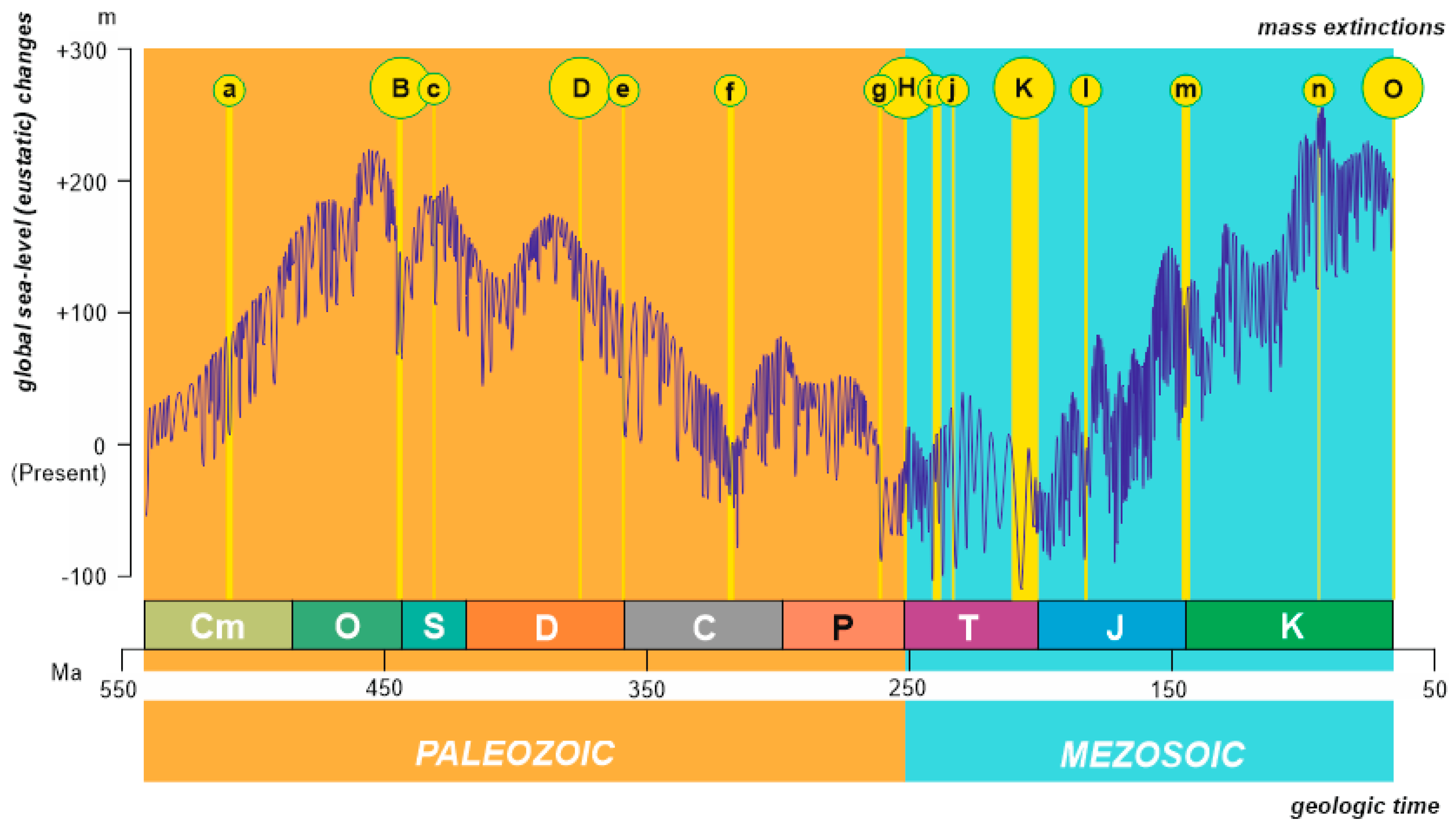
| Label * | Age ** | Status | Key Literature *** |
|---|---|---|---|
| a | mid-Cambrian (end-Series 2) | minor | [40] |
| B | end-Ordovician (Hirnantian) | “Big Five” | [41,42] |
| c | Llandovery/Wenlock | minor | [43] |
| D | Late Devonian (Frasnian/Famennian) | “Big Five” | [44] |
| e | Devonian/Carboniferous | minor | [44] |
| f | mid-Carboniferous (late Serpukhovian) | minor | [45,46] |
| g | end-Guadalupian | potentially major | [47,48] |
| H | end-Permian | “Big Five” | [49,50,51] |
| i | mid-Triassic-1 (Ladinian) | possible | [52] |
| j | mid-Triassic-2 (Carnian) | minor | [53] |
| K | end-Triassic | “Big Five” | [54,55,56] |
| l | Early Jurassic (early Toarcian) | minor | [57,58,59] |
| m | Jurassic/Cretaceous | minor | [60,61] |
| n | Late Cretaceous (late Cenomanian) | minor | [62,63,64] |
| O | end-Cretaceous | “Big Five” | [65] |
| Labels * | Global Sea-Level Changes | |
|---|---|---|
| Hallam and Wignall [17] | This Study | |
| a | not recorded | strong fall and strong rise |
| B | fall and rise | strong falls with strong rise in between |
| c | - | strong fall |
| D | rise | weak fluctuations and strong fall |
| e | rise | strong fall |
| f | - | weak fluctuations |
| g | fall | strong fall |
| H | rise | weak fluctuations |
| i | - | strong rise and weak fluctuations |
| j | - | strong fall |
| K | fall | strong fall, strong rise, and weak fluctuations |
| l | rise | strong rise and strong fall |
| m | - | moderate fluctuations |
| n | rise | weak fluctuations and strong rise |
| O | rise | weak fall |
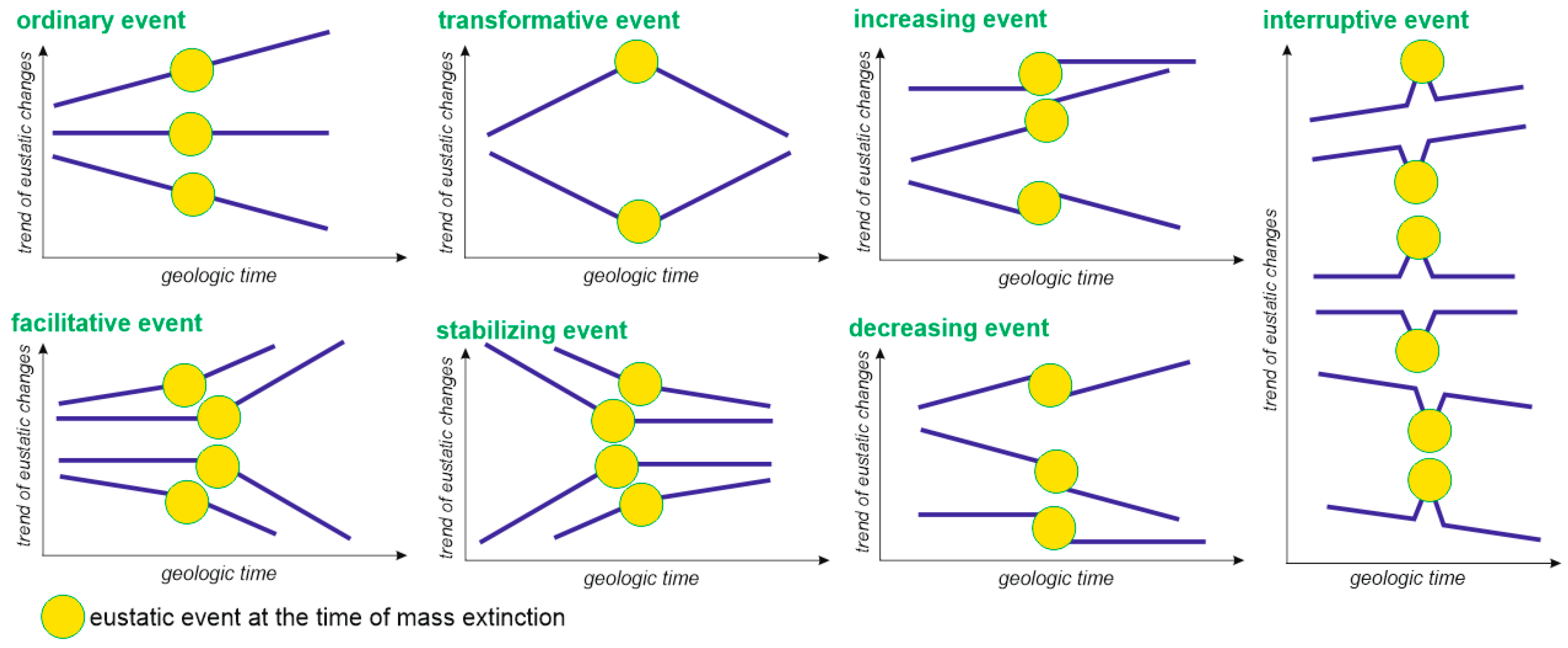
| Labels * | Anomalous | “Short-Term” Record | “Long-Term” Record |
|---|---|---|---|
| a | No | ordinary | ordinary |
| B | Yes | transformative | interruptive |
| c | Yes | decreasing | quasi-interruptive |
| D | Yes | interruptive | interruptive |
| e | Yes/No | interruptive | interruptive |
| f | No | stabilizing | interruptive |
| g | Yes | stabilizing | stabilizing |
| H | No | facilitative | ordinary |
| i | No | ordinary | ordinary |
| j | No | ordinary | ordinary |
| K | Yes | interruptive | interruptive |
| l | Yes | transformative | decreasing |
| m | No | interruptive | interruptive |
| n | No | transformative | transformative |
| O | No | ordinary | ordinary |
Publisher’s Note: MDPI stays neutral with regard to jurisdictional claims in published maps and institutional affiliations. |
© 2020 by the author. Licensee MDPI, Basel, Switzerland. This article is an open access article distributed under the terms and conditions of the Creative Commons Attribution (CC BY) license (http://creativecommons.org/licenses/by/4.0/).
Share and Cite
Ruban, D.A. Paleozoic–Mesozoic Eustatic Changes and Mass Extinctions: New Insights from Event Interpretation. Life 2020, 10, 281. https://doi.org/10.3390/life10110281
Ruban DA. Paleozoic–Mesozoic Eustatic Changes and Mass Extinctions: New Insights from Event Interpretation. Life. 2020; 10(11):281. https://doi.org/10.3390/life10110281
Chicago/Turabian StyleRuban, Dmitry A. 2020. "Paleozoic–Mesozoic Eustatic Changes and Mass Extinctions: New Insights from Event Interpretation" Life 10, no. 11: 281. https://doi.org/10.3390/life10110281
APA StyleRuban, D. A. (2020). Paleozoic–Mesozoic Eustatic Changes and Mass Extinctions: New Insights from Event Interpretation. Life, 10(11), 281. https://doi.org/10.3390/life10110281